HAL Id: hal-01241088
https://hal.inria.fr/hal-01241088
Submitted on 9 Dec 2015HAL is a multi-disciplinary open access
archive for the deposit and dissemination of sci-entific research documents, whether they are pub-lished or not. The documents may come from teaching and research institutions in France or abroad, or from public or private research centers.
L’archive ouverte pluridisciplinaire HAL, est destinée au dépôt et à la diffusion de documents scientifiques de niveau recherche, publiés ou non, émanant des établissements d’enseignement et de recherche français ou étrangers, des laboratoires publics ou privés.
Tight Bounds for Distributed Minimum-Weight
Spanning Tree Verification
Liah Kor, Amos Korman, David Peleg
To cite this version:
Liah Kor, Amos Korman, David Peleg. Tight Bounds for Distributed Minimum-Weight Spanning Tree Verification. Theory of Computing Systems, Springer Verlag, 2013, �10.1007/s00224-013-9479-7�. �hal-01241088�
Tight Bounds For Distributed Minimum-weight Spanning Tree
Verification
Liah Kor ∗ Amos Korman† David Peleg ∗
Abstract
This paper introduces the notion of distributed verification without preprocessing. It focuses on the Minimum-weight Spanning Tree (MST) verification problem and establishes tight upper and lower bounds for the time and message complexities of this problem. Specifically, we provide an MST verification algorithm that achieves simultaneously ˜O(m) messages and ˜O(√n+D) time, where m is the number of edges in the given graph G, n is the number of nodes, and D is G’s diameter. On the other hand, we show that any MST verification algorithm must send ˜Ω(m) messages and incur ˜Ω(√n + D) time in worst case.
Our upper bound result appears to indicate that the verification of an MST may be easier than its construction, since for MST construction, both lower bounds of ˜Ω(m) messages and
˜
Ω(√n+D) time hold, but at the moment there is no known distributed algorithm that constructs an MST and achieves simultaneously ˜O(m) messages and ˜O(√n + D) time. Specifically, the best known time-optimal algorithm (using ˜O(√n + D) time) requires O(m + n3/2) messages, and the best known message-optimal algorithm (using ˜O(m) messages) requires O(n) time. On the other hand, our lower bound results indicate that the verification of an MST is not significantly easier than its construction.
keywords: Distributed algorithms, distributed verification, labeling schemes, minimum-weight spanning tree.
1
Introduction
1.1 Background and Motivation
The problem of computing a Minimum-weight Spanning Tree (MST) received considerable attention in both the distributed setting as well as in the centralized setting. In the distributed setting, constructing such a tree distributively requires a collaborative computational effort by all the network vertices, and involves sending messages to remote vertices and waiting for their replies. This is particularly interesting in the CON GE ST model of computation, where due to congestion constrains, each message can encode only a limited number of bits, specifically, this number is typically assumed to be O(log n), where n denotes the number of nodes in the network. The main measures considered for evaluating a distributed MST protocol are the message complexity, namely,
∗
Department of Computer Science and Applied Mathematics, The Weizmann Institute of Science, Rehovot, 76100 Israel. E-mail: {liah.kor,david.peleg}@weizmann.ac.il. Supported by a grant from the United States-Israel Binational Science Foundation (BSF).
†
CNRS and LIAFA, Univ. Paris 7, Paris, France. E-mail: [email protected]. Sup-ported by the ANR project DISPLEXITY, and by the INRIA project GANG.
the maximum number of messages sent in the worst case scenario, and the time complexity, namely, the maximum number of communication rounds required for the protocol’s execution in the worst case scenario. The line of research on the distributed MST computation problem was initiated by the seminal work of Gallager, Humblet, and Spira [17] and culminated in the O(n) time and O(m + n log n) messages algorithm by Awerbuch [2], where m denotes the number of edges in the network. Both of these algorithms apply also to asynchronous systems. As pointed out in [2], the results of [4, 6, 15] establish an Ω(m + n log n) lower bound on the number of messages required to construct a MST. Thus, the algorithm of [2] is essentially optimal.
This was the state of affairs until the mid-nineties when Garay, Kutten, and Peleg [18] initiated the analysis of the time complexity of MST construction as a function of additional parameters (other than n), and gave the first sublinear time distributed algorithm for the MST problem, running in time O(D + n0.614), where D is the diameter of the network. This result was later improved to O(D +√n log∗n) by Kutten and Peleg [29]. The tightness of this latter bound was shown by Peleg and Rubinovich [32] who proved that ˜Ω(√n) is essentially1 a lower bound on the time for constructing MST on graphs with diameter Ω(log n). This result was complemented by the work of Lotker, Patt-Shamir and Peleg [31] that showed an ˜Ω(√3n) lower bound on the time required for
MST construction on graphs with small diameter. Note, however, that the time-efficient algorithms of [18, 29] are not message-optimal, i.e., they take asymptotically much more than O(m + n log n) messages. For example, the time-optimal protocol of [29] requires sending O(m + n3/2) messages. The question of whether there exists an optimal distributed algorithm for MST construction that achieves simultaneously ˜O(m) messages and ˜O(√n + D) time still remains open.
This paper addresses the MST verification problem in the CON GE ST model. Informally, the setting we consider is as follows. A subgraph is given in a distributed manner, namely, some of the edges incident to every vertex are locally marked, and the collection of marked edges at all the vertices defines a marked subgraph; see, e.g., [7, 17, 26, 27]. The verification task requires checking distributively whether the marked subgraph is indeed an MST of the given graph. Similarly to the papers dealing with sub-linear time MST construction [18, 29], we consider a synchronous environment.
1.2 Our Results
We consider the MST verification problem and establish asymptotically tight upper and lower bounds for the time and message complexities of this problem. Specifically, in the positive direction we show the following:
Theorem 1.1 There exists a distributed MST verification algorithm that uses ˜O(√n + D) time and ˜O(m) messages.
This result appears to indicate that MST verification may be easier than MST construction, since, at the moment, it is not known whether there exists an algorithm that constructs an MST simultaneously in ˜O(√n + D) time and ˜O(m) messages. Conversely, we show that the verification problem is not much easier than the construction, by proving that the known lower bounds for MST construction also hold for the verification problem. Specifically, we prove the following two matching lower bounds.
Theorem 1.2 Any distributed algorithm for MST verification requires Ω(m) messages.
Theorem 1.3 Any distributed algorithm for MST verification requires ˜Ω(√n + D) time.
To the best of our knowledge, this paper is the first to investigate distributed verification without assuming any kind of preprocessing (see Section 1.3.2). Following this paper, several other works on distributed verification have already been published. More specifically, a systematic study of distributed verification is established for various verification tasks [8]. Distributed verification in the LOCAL model has been studied in [13, 14], mostly focusing on computational complexity issues.
Our ˜Ω(√n + D) time lower bound for verifying an MST is achieved by a (somewhat involved) modification of the corresponding lower bound for the computational task [32]. The idea behind our time lower bound was already found useful in several continuation studies. Specifically, a modification of our proof technique was used in [8] to yield time lower bounds for several other verification tasks, and for establishing a lower bound on the hardness of approximating an MST. Somewhat surprisingly, in [9], the proof technique was extended even further to yield a result in the (seemingly unrelated) area of distributed random walks.
1.3 Other related work
1.3.1 MST computation and verification in the centralized setting
In the centralized setting, there is a large body of literature concerning the problem of efficiently computing an MST of a given weighted graph. Reviews can be found, e.g., in the survey paper by Graham and Hell [19] or in the book by Tarjan [36] (Chapter 6). The fastest known algorithm for finding an MST is that of Pettie and Ramachandran [33], which runs in O(m · α(m, n)) time, where α is the inverse Ackermann function, n is the number of vertices and m is the number of edges in the graph. Unfortunately, a linear (in the number of edges) time algorithm for computing an MST is known only in certain cases, or by using randomization [16, 21].
The separation between computation and verification, and specifically, the question of whether verification is easier than computation, is a central issue of profound impact on the theory of computer science. In the context of MST, the verification problem (introduced by Tarjan [35]) is the following: given a weighted graph, together with a subgraph, it is required to decide whether this subgraph forms an MST of the graph. At the time it was published, the running time of the MST verification algorithm of [35] was indeed superior to the best known bound on the computational problem. Improved verification algorithms in different centralized models were then given by Harel [20], Koml`os [25], and Dixon, Rauch, and Tarjan [10], and parallel algorithms were presented by Dixon and Tarjan [11] and by King, Poon, Ramachandran, and Sinha [24]. Even though it is not known whether there exists a deterministic algorithm that computes an MST in O(m) time, the verification algorithm of [10] is in fact linear, i.e., runs in time O(m) (the same result with a simpler algorithm was later presented by King [23] and by Buchsbaum [5]). For the centralized setting, this may indicate that the verification of an MST is indeed easier than its computation.
1.3.2 Distributed verification with preprocessing
Some previous papers investigated distributed verification tasks assuming that the algorithm de-signer can perform a preprocessing stage to help the verification, cf. [1, 3, 12, 26, 27]. Typically, in this preprocessing stage, data structures (i.e., labels, proofs) are provided to the nodes of the graph, and using these data structures, the verification proceeds in a constant number of rounds. The focus in those studies was on the minimum size of a data structure (i.e., amount of information
stored locally), while the complexities of the preprocessing stage providing the data structures were not analyzed.
2
Preliminaries
2.1 The Model
A point-to-point communication network is modeled as an undirected graph G(V, E), where the vertices in V represent the network processors and the edges in E represent the communication links connecting them. We denote by n the number of vertices in G, i.e., n = |V |, and let m denote the number of edges, i.e., m = |E|. The length of a path in G is the number of edges it contains. The distance between two vertices u and v is the length of the shortest path connecting them. The diameter of G, denoted D, is the maximum distance between any two vertices of G.
Vertices are assumed to have unique identifiers, and each vertex v knows its own identifier ID(v). A weight function ω : E → N associated with the graph assigns a nonnegative integer weight ω(e) to each edge e = (u, v) ∈ E. The vertices do not know the topology or the edge weights of the entire network, but they know the weights of the edges incident to them, that is, the weight ω((u, v)) is known to u and v. Similarly to corresponding works on MST computation, we assume that the edge weights are bounded by a polynomial in n (this assumption implies that a weight of an edge can be encoded using O(log n) bits, and hence can be encoded in one message).
Similarly to previous work, we consider the CON GE ST model. Specifically, the vertices can communicate only by sending and receiving messages over the communication links. Each vertex can distinguish between its incident edges. Moreover, if vertex v sends a message to vertex u along the edge e = (v, u), then upon receiving the message, vertex u knows that the message was delivered over the edge e. At most one O(log n) bits can be sent on each link in each message. Similarly to [18, 29], we assume that the communication is carried out in a synchronous manner, i.e., all the vertices are driven by a global clock. Messages are sent at the beginning of each round, and are received at the end of the round. (Clearly, our lower bounds hold for asynchronous networks as well.) Relevant studies typically assume that computations start either at a single source node or simultaneously at all nodes. Our results hold for both of these settings.
2.2 The distributed MST Verification problem
Formally, the minimum-weight spanning tree (MST) verification problem can be stated as follows. Given a graph G(V, E), a weight function ω on the edges, and a subset of edges T ⊆ E, referred as the MST candidate, it is required to decide whether T forms a minimum spanning tree on G, i.e., a spanning tree whose total weight ω(T ) = P
e∈Tω(e) is minimal. In the distributed model, the
input and output of the MST verification problem are represented as follows. Each vertex knows the weights of the edges connected to its immediate neighbors. A degree-d vertex v ∈ V with neighbors u1, . . . , udhas d weight variables W1v, . . . , Wdv, with Wiv containing the weight of the edge
connecting v to ui, i.e., Wiv = ω(v, ui), and d boolean indicator variables Y1v, . . . , Ydv indicating
which of the edges adjacent to v participate in the MST candidate that we wish to verify. The indicator variables must be consistent, namely, for every edge (u, v), the indicator variables stored at u and v for this edge must agree (this is easy to verify locally). Let TY be the set of edges
marked by the indicator variables (i.e., all edges for which the indicator variable is set to 1). The output of the algorithm at each vertex v is an assignment to a (boolean) output variable Av that
must satisfy Av = 1 if TY is an MST of G(V, E, ω), and Av = 0 otherwise.
3
An MST Verification Algorithm
In this section we describe our MST verification algorithm, prove its correctness and analyze its time and message complexities.
First, we note that in this section we assume that the verification algorithm is initiated by a designated source node. The case in which all nodes wake up simultaneously can be reduced to the single source setting using the leader election algorithm of [30], which employs ˜O(m) messages and runs in ˜O(D) time.
3.1 Definitions and Notations
Following are some definitions and notations used in the description of the algorithm. For a graph G = (V, E, ω), an edge e is said to be cycle-heavy if there exists a cycle C in G that contains e, and e has the heaviest weight in C. For a graph G = (V, E, ω), a set of edges F ⊆ E is said to be an MST fragment of G if there exists a minimum spanning tree T of G such that F is a subtree of T (i.e., F ⊆ T and F is a tree). Similarly, a collection F of edge sets is referred to as an MST fragment collection of G if there exists an MST T of G such that (1) Fi is a subtree of T for every
Fi ∈ F , (2)SFi∈FV (Fi) = V , and (3) V (Fi) ∩ V (Fj) = ∅ for every Fi, Fj ∈ F , where i 6= j.
Consider a graph G = (V, E, ω), an MST fragment collection F , a subgraph T of G and a vertex v in G. The fragment graph of G, denoted GF, is defined as a graph whose vertices are
the MST fragments Fi ∈ F , and whose edge set contains an edge (Fi, Fj) if and only if there exist
vertices u ∈ V (Fi) and v ∈ V (Fj) such that (u, v) ∈ E. Similarly, the fragment graph induced by T ,
denoted TF, is defined as a graph whose vertices are the MST fragments Fi ∈ F , and whose edge
set contains an edge (Fi, Fj) for i 6= j if and only if there exist vertices u ∈ V (Fi) and v ∈ V (Fj)
such that (u, v) ∈ T . The edges of TF are also referred to as the inter-cluster edges induced by T .
For each vertex v, let ET(v) denote the set of edges of T incident to v. For each fragment
F ∈ F , the set of fragment internal edges of F induced by T , denoted EF,T, consists of all edges of
T with both endpoints in V (F ), i.e., EF,T = {e | e = (u, v) ∈ T and u, v ∈ V (F )}. The fragment
of v, denoted by F (v), is the fragment F ∈ F such that v ∈ V (F ). Denote by EF(v) the set of
edges in F (v) that are incident to v (i.e., EF(v) = {e| e = (u, v) ∈ E and u ∈ V (F (v))}). Similarly,
denote by EF,T(v) the set of fragment internal edges of F induced by T and incident to v.
Throughout the description of the verification algorithm we assume that the edge weights are distinct. Having distinct edge weights simplifies our arguments since it guarantees the uniqueness of the MST. Yet, this assumption is not essential. Alternatively, in case the graph is not guaranteed to have distinct edge weights, we may use a modified weight function ω0(e), which orders edge weights lexicographically. At this point we would like to note that the standard technique (e.g., [17]) for obtaining unique weights is not sufficient for our purposes. Indeed, that technique orders edge weights lexicographically: first, by their original weight ω(e), and then, by the identifiers of the edge endpoints (say, first comparing the smaller of the two identifiers of the endpoints, and then the larger one). This yields a modified graph with unique edge weights, and an MST of the modified graph is necessarily an MST of the original graph. For construction purposes it is therefore sufficient to consider only the modified graph. However, this is not the case for verification purposes, as the given subgraph can be an MST of the original graph but not necessarily an MST
of the modified graph.
While we cannot guarantee than any MST of the original graph is an MST of the modified graph (having unique edge weights), we make sure that the particular given subgraph T is an MST of the original graph if and only if it is an MST of modified one. This condition is sufficient for our purposes, and allows us to consider only the modified graph. Specifically, to obtain the modified graph, we employ a slightly different technique than the classical one. That is, edge weights are lexicographically ordered as follows. For an edge e = (v, ui) connecting v to its ith neighbor ui,
consider first its original weight ω(e), next, the value 1 − Yiv where Yiv is the indicator variable of the edge e (indicating whether e belongs to the candidate MST to be verified), and finally, the identifiers of the edge endpoints, ID(v) and ID(ui) (say, first comparing the smaller of the two
identifiers of the endpoints, and then the larger one). Formally, let
ω0(e) = hω(e), 1 − Yiv, IDmin(e), IDmax(e)i ,
where IDmin(e) = min{ID(v), ID(ui)} and IDmax(e) = max{ID(v), ID(ui)}. Under this weight
function ω0(e), edges with indicator variable set to 1 will have lighter weight than edges with the same weight under ω(e) but with indicator variable set to 0 (i.e., for edges e1∈ T and e2 ∈ T such/
that ω(e1) = ω(e2), we have ω0(e1) < ω0(e2)). It follows that the given subgraph T is an MST of
G(V, E, ω) if and only if T is an MST of G(V, E, ω0). Moreover, since ω0(·) takes into account the unique vertex identifiers, it assigns distinct edge weights.
The MST verification algorithm makes use of Procedures DOM Part and MAX Label, presented in [29] and [22] respectively. Before we continue, let us first recall what these procedures guarantee.
Procedure DOM Part: The distributed Procedure DOM Part, used in [29], partitions a given graph into an MST fragment collection (MFC) F , where each fragment is of size at least k + 1 and depth O(k), for a parameter k to be specified later (aiming to optimize the total costs). A fragment leader vertex is associated with each constructed fragment (the identifier of the fragment is defined as the identifier of the fragment’s leader). After Procedure DOM Part is completed, each vertex v knows the identifier of the fragment to which it belongs and v’s incident edges that belong to the fragment. (To abide by the assumption of [29] that each vertex knows the identifiers of its neighbors, before applying Procedure DOM Part, the algorithm performs a single communication round that exchanges vertex identifiers between neighboring vertices.) The execution of Procedure DOM Part, requires O(k · log∗n) time and O(m · log k + n · log∗n · log k) messages. The parameter k to be used by our protocol, chosen as a suitable breakpoint so as to optimize the total costs, satisfies k = Θ(√n + D), hence, our invocation of Procedure DOM Part will require ˜O(√n + D) time and ˜O(m) messages.
The MAX Label labeling scheme: The labeling scheme MAX Label of [22] is a centralized proce-dure designed for the family of weighted trees. The proceproce-dure involves two components: an encoder algorithm E and a decoder algorithm D. These two components satisfy the following.
1. Given a weighted tree T , the encoder algorithm E assigns a label L(v) to each vertex v of T .
2. Given two labels L(u) and L(v) assigned by E to two vertices u and v in some weighted tree T , the decoder algorithm D outputs M AX(u, v), which is the maximum weight of an edge on the path connecting u and v in T . (The decoder algorithm D bases its answer on the pair of labels L(u) and L(v) only, without knowing any additional information regarding the tree T .)
The labeling scheme MAX Label produces O(log n log W )-bit labels, where W is the largest weight of an edge. Since W is assumed to be polynomial in n, the label size is O(log2n) bit.
3.2 The algorithm
Overview: The algorithm consists of three phases. The first phase starts by letting the source node s construct a BFS tree rooted at s, and calculating the values of the number of nodes n and a 2-approximation d to the diameter D of the graph. Then, the distributed Procedure DOM Part of [29] in invoked with parameter k = max{√n, d} = Θ(√n+D), where D is the diameter of the graph. This procedure constructs an MST fragment collection (MFC) F , where every fragment in F is of size at least k + 1 and depth O(k). As mentioned, our invocation of Procedure DOM Part requires
˜
O(√n + D) time and ˜O(m) messages. The algorithm verifies that the set of edges contained in the constructed MFC is equal to the set of fragment internal edges induced by the MST candidate T , i.e.,S
F ∈FE(F ) =
S
F ∈FEF,T (this verifies that each F ∈ F is contained in T and that T does not
contain additional fragment internal edges.) Note that this is a necessary condition for correctness since the graph is assumed to have a unique MST.
In the following phases, the algorithm verifies that all remaining edges of T form an MST on the fragment graph GF. Let TF be the fragment graph induced by T with respect to the MFC F
found in the previous phase. In order to verify that TF forms an MST on the fragment graph GF,
it suffices to verify that TF is a tree and that none of the edges of TF is a cycle heavy edge in GF.
The above is done as follows.
In the second phase, the structure of TF is aggregated over the BFS tree to the source node
s, which in turn verifies that TF is indeed a tree. Note that this aggregation is not very wasteful,
and requires O(D + f ) time and O(D · f ) messages, where f is the number of nodes in TF. As
shown later, f ≤ n/k, and hence, this aggregation can be done using ˜O(√n + D) time and ˜O(m) messages.
In the third phase, the source node s employs the (centralized) labeling scheme MAX Label of [22] (or [26]) on TF. Informally, the labeling scheme assigns a label L(Fi) to each vertex Fi of TF using
the encoder algorithm E applied on TF. The label L(Fi) is then efficiently delivered to each vertex
in Fi. More specifically, the f labels are broadcasted over the BFS tree, so that eventually, each
node in a fragment knows its corresponding label. This broadcasts costs ˜O(D + f ) = ˜O(√n + D) time and ˜O(D · f ) = ˜O(m) messages. Recall, that given the labels of two fragments L(Fi) and
L(Fj) it is now possible to compute the weight of the heaviest edge on the path connecting the
fragments in TF by applying the decoder algorithm D. Once all vertices obtain the labels of their
corresponding fragments, each vertex of G can verify (using the decoder D) by communicating with its neighbors only, that each inter fragment edge incident to it and not participating in TF forms a
cycle when added to TF for which it is a cycle heavy edge. Following is a more detailed description
of the algorithm.
1. Phase 1
(a) The source node s (which initiates the algorithm) constructs a BFS tree rooted at s, computes the values n and d, where n is the number of nodes and d is the depth of the BFS tree. (Note that d is a 2-approximation to the diameter D of the graph.) Subsequently, the source node s broadcasts a signal over the BFS tree containing the values n and d and instructing each vertex to send its identifier to all its neighbors.
This guarantees that all nodes know the values of n and d as well as the identifiers of their neighbors. In addition, to start the next step (i.e., Step 2.b) at the same time, the broadcast is augmented with a counter that is initialized by the source s to d + 1 is decreased by one when delivered to a child in the BFS tree. Let c(u) denote the counter received at node u. Before starting the next step each node u waits for c(u) rounds after receiving the counter.
(b) Perform Procedure DOM Part(k), with parameter k = max{√n, d} = Θ(√n + D). The result is an MFC F , where each fragment F ∈ F is of size |V (F )| > k and depth O(k), having a fragment leader and a distinct fragment identifier known to all vertices in the fragment.
(c) Each vertex sends its fragment identifier to all its neighbors.
(d) By comparing the fragment identifiers of its neighbors with its own fragment identifier, each vertex v identifies the sets of edges EF(v) and EF,T(v).
(e) Verify that S
F ∈FE(F ) =
S
F ∈FEF,T by verifying at each vertex v that EF(v) =
EF,T(v). (Else return “T is not an MST”.)
2. Phase 2
(a) Vertex s counts the number of fragments, denoted by f . This is implemented by letting s broadcast a signal over the BFS tree instructing the nodes to perform a convergecast over the BFS tree. During this convergecast the number of fragments is aggregated to the root s by letting only fragment leader vertices increase the fragment counter. This guarantees that the fragment counter at the root s is f .
(b) Vertex s counts the number of inter fragment edges induced by T (i.e., the number of edges in TF) by performing another convergecast over the BFS tree. Then, s verifies
that the number of edges is equal to f − 1. (Else return “T is not an MST”.)
(c) Vertex s broadcasts a signal over the BFS tree instructing all vertices to send the descrip-tion of all their incident edges in TF to s, by performing a convergecast over the BFS
tree. (The edges of TF are all edges of T that connect vertices from different fragments.)
(d) Vertex s verifies that TF is a tree. (Else return “T is not an MST”.)
3. Phase 3
(a) Each fragment leader sends a message to vertex s over the BFS tree. Following these messages, all vertices save routing information regarding the fragment leaders. I.e., if v is a fragment leader and v is a descendant of some other vertex u in the BFS tree, then, after this step is applied, u knows which of its children is on the path connecting it to the fragment leader v.
(b) Vertex s computes the labels L(F ) for all vertices F in TF (i.e., assigns a label to each of
the fragments) using the encoder algorithm E . Subsequently, s sends to each fragment leader its fragment label (the label of each fragment is sent to the fragment leader over the BFS tree using the routing information established in Step 3a above). (Recall that each label is encoded using O(log2n) bits.)
(c) Each fragment leader broadcasts its fragment label to all vertices in the fragment. The broadcast is done over the fragment edges.
(d) Each vertex v sends its fragment label to all its neighbors in other fragments. (Recall that v already knows EF(v) by step 1d.)
(e) Each vertex v verifies, for every neighbor u such that u does not belong to v0s fragment and (u, v) /∈ T , that ω(v, u) ≥ M AX(F (v), F (u)). (The value M AX(F (v), F (u)) is computed by applying the decoder algorithm D to the labels L(F (v)) and L(F (u)).) (Else return “T is not an MST”.)
3.3 Correctness
We now show that our MST verification algorithm correctly identifies whether the given subgraph T is an MST. We begin with the following claim.
Claim 3.1 Let T be a spanning tree of G such that T contains all edges of the MFC F and TF
forms an MST on the fragment graph of G (with respect to the MFC F ). Then T is an MST on G. Proof Since F is an MST fragment collection, there exists an MST T0 of G such that T0 contains all edges of F . Due to the minimality of T0, the fragment graph TF0 induced by T0 necessarily forms an MST on GF, the fragment graph of G. Hence we get that ω(T ) = ω(T0), thus T is an MST
of G.
Due to the assumption that edge weights are distinct, we get: Observation 3.2 The MST of G is unique.
By combining Claim 3.1 and Observation 3.2 we get the following.
Claim 3.3 A spanning tree T of G is an MST if and only if T contains all edges of the MFC F and TF forms an MST on GF.
Lemma 3.4 The MST verification algorithm correctly identifies whether the given tree T is an MST of the graph G.
Proof By Claim 3.3, to prove the correctness of the algorithm it suffices to show that given an MST candidate T , the algorithm verifies that:
(1) T is a spanning tree of G,
(2) T contains all edges of F , and
(3) TF forms an MST on GF.
Since F as constructed by Procedure DOM Part in the first phase is an MFC, it spans all vertices of G. Step 1e verifies thatS
F ∈FE(F ) =
S
F ∈FEF,T, thus after this step, it is verified that T does
not contain a cycle that is fully contained in some fragment F ∈ F (since every F ∈ F is a tree). On the other hand, step 2d verifies that T does not contain a cycle that contains vertices from different fragments. Hence, the algorithm indeed verifies that T is a spanning tree of G, and Property (1) follows. Property (2) is clearly verified by step 1e of the algorithm. Finally, to verify that TF forms
an MST on the fragment graph of G it suffices to verify that inter-fragment edges not in TF are
3.4 Complexity
Consider first the Phase 1. Steps 1a and 1c clearly take O(D) time and O(m) messages. Step 1b, i.e., the execution of Procedure DOM Part, requires O(k · log∗n) time and O(E · log k + n · log∗n · log k) messages. (A full analysis appears in [34].) The remaining steps of the first phase are local computations performed by all vertices. Thus, since k is set to k = Θ(√n + D), the first phase of the MST verification algorithm requires requires ˜O(√n + D) time and ˜O(m) messages.
Observe now, that since the fragments are disjoint and each fragment contains at least k vertices, we have the following.
Observation 3.5 The number of MST fragments constructed during the first phase of the algo-rithm is f ≤ n/k = O(min{√n,Dn}).
The first two steps of phase 2, namely, steps 2a and 2b consist of simple broadcasts over the BFS tree, hence they require O(D) time and O(m) messages. Step 2c consists of upcasting all the edges in TF to s. Note that the number of edges in TF can potentially be as high as m. However,
given that the verification did not fail in Step 2b, we are guaranteed that the number of edges in TF is f − 1. Thus, Step 2c amounts to upcasting f − 1 messages and can therefore be performed
in O(D + f ) time and O(f D) messages. Step 3a consists of an upcast of f messages over the BFS tree and thus requires the same time and message complexities as that of step 2c. Step 3b consists of a BFS downcast of f messages (each of size log2n); it therefore requires O(D + f log n) time and O(f D log n) messages. Step 3c consists of a broadcast of a label (of size O(log2n)) in each of the MST fragments; this can be performed in O(k + log n) time and O(n log n) messages. Finally, step 3d can be performed in O(log n) time and O(m log n) messages, and step 3e amounts to local computations. Table 1 below summarizes the time and message complexities of the second and third phases of the algorithm.
Step Description Time Messages
2a,2b BFS convergecast O(D) O(m)
2c, 3a BFS upcast of f messages O(D + f ) O(f · D)
2d,3e Local computation 0 none
3b BFS downcast of f messages (each of size log2n) O(D + f · log n) O(f · log n · D) 3c Broadcast in each of the MST fragments O(k + log n) O(n · log n)
3d Communication between neighbors O(log n) O(log n · m)
Table 1: Time and message complexities of phases 2 and 3 of the algorithm. D is the diameter of the graph, and f is the number of MST fragments constructed in phase 1.
Combining the above arguments, and using the fact that f = O(min{√n,Dn}) (see Observation 3.5), we obtain the following.
Lemma 3.6 The algorithm describes above requires ˜O(√n + D) time and ˜O(m) messages. Theorem 1.1 follows by combining the lemma above with Lemma 3.4.
4
Time Complexity Lower Bound
In this section, we prove an ˜Ω(√n + D) lower bound on the time required to solve the MST verification. Clearly, Ω(D) time is inevitable in the case of a single source node. The case in which
all nodes start at the same time is also very simple. Indeed, in this case, the Ω(D) time bound follows by considering a cycle C of size n with all edges having weight 1 except for two edges e and e0 located at opposite sides. The given candidate spanning tree is T = C \ {e}. The two edges e and e0 can have arbitrary weights, hence, to decide whether T is an MST one needs to transfer information along at least half of the cycle. This shows a lower bound of Ω(D) for the case where D = Θ(n). A similar argument can be applied for arbitrary values of D.
The difficult part is to prove a time lower bound of ˜Ω(√n). We prove this lower bound for the case where all nodes start at the execution at the same time. The lower bound for the case of a single source node follows directly from this lower bound, relying on the leader election algorithm of [30], which runs in ˜O(D) time.
In the remaining of this section we consider the case where all nodes start the execution simul-taneously at the same time, and prove a lower bound of ˜Ω(√n). To show the lower bound, we first define a new problem named vector equality, and then show a lower bound for the time required to solve it. This is established in Section 4.1. More specifically, for the purposes of this lower bound proof, we consider the collection of graphs denoted Fm2, for m ≥ 2, as defined in [32]. Each graph graph F2
m consists of n = Θ(m4) vertices, and its diameter is Θ(m). In Section 4.1.2, we establish
a time lower bound of ˜Ω(m2) = ˜Ω(√n) for solving vector equality in each graph Fm2.
In Section 4.2, for m ≥ 2, we consider a family Jm2 of weighted graphs (these are weighted versions of the graph Fm2), and show that any algorithm solving the MST verification problem on the graphs in J2
m can also be used to solve the vector equality problem on Fm2 with the same
time complexity. This establishes the desired ˜Ω(√n) time lower bound for the distributed MST verification problem.
4.1 A lower bound for the vector equality problem
The vector equality problem EQ(G, s, r, b). Consider a graph G and two specified distinguished vertices s and r, each storing b boolean variables, ¯Xs = hX1s, . . . , Xbsi and ¯Xr = hX1r, . . . , Xbri respectively, for some integer b ≥ 1. An instance of the problem consists of initial assignments
¯
Xs = {Xis| 1 ≤ i ≤ b} and ¯Xr= {Xir | 1 ≤ i ≤ b}, where Xs
i, Xir ∈ {0, 1}, to the variables of s and
r respectively. Given such an instance, the vector equality problem requires r to decide whether ¯
Xs = ¯Xr, i.e., Xis= Xir for every 1 ≤ i ≤ b.
4.1.1 The graphs Fm2
Let us recall the collection of graphs denoted Fm2, for m ≥ 2, as defined in [32]. (See Figure 1). The components used are the ordinary path P on m2 + 1 vertices, where V (P) = {v0, . . . , vm2},
E(P) = {(vi, vi+1) | 0 ≤ i ≤ m2− 1}, and the highway H on m + 1 vertices, where V (H) = {him|
0 ≤ i ≤ m} and E(H) = {(him, h(i+1)m) | 0 ≤ i ≤ m − 1}. Each highway vertex him is connected
to the corresponding path vertex vimby a spoke edge (him, vim).
The graph Fm2 is constructed of m2 copies of the path, P1, . . . , Pm2, and connecting them to the highway H. The two distinguished vertices are s = h0 and r = hm2. The spoke edges are
grouped into m + 1 stars Si, 0 ≤ i ≤ m, with each Si consisting of the vertex him and the m2
vertices vim1 , . . . , vimm2 connected to it by spoke edges. Hence V (Si) = {him} ∪ {vim1 , . . . , vm
2
im} and
E(Si) = {(vjim, him) | 1 ≤ j ≤ m2}. The graph Fm2 consists of V (Fm2) = V (H) ∪
Sm2
j=1V (Pj) and
E(Fm2) =Sm
i=0E(Si) ∪
Sm2
4.1.2 The lower bound for EQ
Our goal now is to prove that solving the vector equality problem on Fm2 with a b = m2-bit input strings ¯Xs, ¯Xrrequires Ω(m2/B) time, assuming each message is encoded using B bits. (Later, we shall take B = O(log n).)
Consider some arbitrary algorithm AEQ, and let ϕ( ¯Xs, ¯Xr) denote the execution of AEQ on
m2-bit inputs ¯Xs, ¯Xr on the graph Fm2. For simplicity, we assume that m2/2 is an integer. For 1 ≤ i ≤ m2/2, define the i-middle set of the graph Fm2, denoted Mi, as follows. For every 1 ≤ j ≤ m2,
define the i-middle of the path Pj as Mi(Pj) = {vlj | i ≤ l ≤ m2− i}. Let β(i) denote the least
integer δ such that δm ≥ i and γ(i) denote the largest integer κ such that κm ≤ m2− i. Define the i-middle of H as Mi(H) = {hjm | β(i) ≤ j ≤ γ(i)}. Now, the i-middle set of Fm2 is the union
of those middle sets, Mi = Mi(H) ∪SjMi(Pj). (See Fig. 1.) For i = 0, the definition is slightly
different, letting M0 = V \ {h0, hm2}.
M
iP
1 h s = 0H
P
m2P
2 h` (i) m vi1 i v2 vmi2 mm2-i 2 m2-i m2-i v v2 1 v ha(i) m r = hm2Figure 1: The middle set Mi in the graph Fm2
Denote the state of the vertex v at the beginning of round t during the execution ϕ( ¯Xs, ¯Xr) on the input ¯Xs, ¯Xr by σ(v, t, ¯Xs, ¯Xr). Without loss of generality, we may assume that in two different executions ϕ( ¯Xs, ¯Xr) and ϕ( ¯X0s, ¯X0r), a vertex reaches the same state at time t, i.e.,
σ(v, t, ¯Xs, ¯Xr) = σ(v, t, ¯X0s, ¯X0r), if and only if it receives the same sequence of messages on each
of its incoming links; for different sequences, the states are distinguishable.
For a given set of vertices U = {v1, . . . , vl} ⊆ V , a configuration C(U, t, ¯Xs, ¯Xr) is a vector
hσ(v1, t, ¯Xs, ¯Xr), . . . , σ(vl, t, ¯Xs, ¯Xr)i of the states of the vertices of U at the beginning of round
t of the execution ϕ( ¯Xs, ¯Xr). Denote by C[U, t] the collection of all possible configurations of the subset U ⊆ V at time t over all executions ϕ( ¯Xs, ¯Xr) of algorithm AEQ (i.e., on all legal inputs
¯
Xs, ¯Xr), and let ρ[U, t] = |C[U, t]|.
Prior to the beginning of the execution (i.e., at the beginning of round t = 0), the input strings ¯
Xs, ¯Xr are known only to vertices s and r respectively. The rest of the vertices are found in some initial state, described by the configuration Cinit = C(M0, 0, ¯Xs, ¯Xr), which is independent
of ¯Xs, ¯Xr. Thus in particular ρ[M0, 0] = 1. (Note, however, that ρ[V, 0] = 22m
2
.) Lemma 4.1 For every 0 ≤ t < m2/2, ρ[Mt+1, t + 1] ≤ (2B+ 1)2· ρ[Mt, t].
Proof The lemma is proved by showing that in round t + 1 of the algorithm, each configuration in C[Mt, t] branches off into at most (2B+ 1)2 different configurations of C[Mt+1, t + 1].
Fix a configuration ˆC ∈ C[Mt, t], and let δ = β(t + 1) and κ = γ(t + 1). The (t + 1)-middle set
Mt+1 is connected to the rest of the graph by the highway edges fδ−1 = (h(δ−1)m, hδm) and fκ =
(hκm, h(κ+1)m) and by the 2m2 path edges ejt = (v j t, v j t+1),e j m2−t = (v j m2−t, v j m2−t+1) 1 ≤ j ≤ m2. (See Fig. 2.) m2-t m2-t+1 m2-t+1 2 m -t -t+1 2 m m2 m2-t m vt2 vt+1m2 1 t v 2 t v vt+12 1 t+1 v b h m r = hm2 1 v v2 2 v m v 2 v v1 g h m
M
t+1P
P
2H
P
1 m2 h0 s =Figure 2: The edges entering the middle set Mt+1.
Let us count the number of different configurations in C[Mt+1, t + 1] that may result of the
configuration ˆC. Starting from the configuration ˆC, each vertex vtj is restricted to a single state, and hence it sends a single (well determined) message over the edge ejt to vjt+1thus not introducing any divergence in the execution. Similarly, each vertex vmj 2−t+1 is restricted to a single state, and
hence it sends a single message over the edge ejm2−t to v
j
m2−t. The same applies to all the edges
internal to Mt+1. As for the highway edges fδ−1, fκ, the vertices h(δ−1)mand h(κ+1)mare not in the
set Mt, hence they may be in any one of many possible states, and the values passed over these edges
into the set Mt+1 are not determined by the configuration ˆC. However, due to the restriction of the
B-bounded-message model, at most (2B+1) different behaviors of fδ−1can be observed by hδmand
at most (2B+1) different behaviors of fκcan be observed by hκm. Thus altogether, the configuration
ˆ
C branches off into at most (2B+ 1)2possible configurations ˆC
1, . . . , ˆC22B+1∈ C[Mt+1, t + 1], differing
only by the states σ(hδm, t + 1, ¯Xs, ¯Xr), σ(hκm, t + 1, ¯Xs, ¯Xr). The lemma follows.
Applying Lemma 4.1 and the fact that ρ[M0, 0] = 1, we get the following result.
Corollary 4.2 For every 0 ≤ t ≤ m2/2, ρ[Mt, t] ≤ (2B+ 1)2t.
To prove the time lower bound for the vector equality problem we introduce the following restricted model of computation as defined in [28]. A two party communication model consists of parties PA and PB connected via a bidirectional communication link. Let SX, SY, SZ be arbitrary
finite sets. We say that Protocol Π computes function f : SX × SY → SZ if, when given input
a ∈ SX known to party PA and input b ∈ SY known to party B, the parties are able to determine
f (a, b) by a sequence of bit exchanges. The following observation follows from [28, 1.14], and is used to prove Lemma 4.4.
Observation 4.3 Consider a protocol Π. Suppose that there exist inputs a, a0 ∈ Sx for party PA and b, b0 ∈ SY for party PB for which in the executions of Π on input (a, b) and on input
(a0, b0), identical sequences of bits are exchanged by both parties. Then the same sequence of bits is exchanged in the execution of Π on input (a0, b).
Lemma 4.4 For every m ≥ 1, solving the vector equality problem EQ(Fm2, h0, hm2, m2) requires
Ω(m2/B) time.
Proof Assume, towards contradiction, that there exists a protocol Π that correctly solves EQ(Fm2, h0, hm2, m2) and has worst case time complexity TΠ < m
2
2B. Let MTΠ be the middle set
of Fm2, as previously defined, corresponding to i = TΠ. Let LTΠ be the set of vertices that reside on
the left side of MTΠ in F
2
mand RTΠ be the set of vertices that reside on the right side of MTΠ. Note
that MTΠ∪ LTΠ∪ RTΠ = V and MTΠ∩ LTΠ = MTΠ∩ RTΠ = LTΠ∩ RTΠ = φ. Consider a simulation
of protocol Π by two parties PA and PB. The simulation works so that party PA simulates the
execution of Π in MTΠ and in LTΠ, and party PB simulates the execution of Π in MTΠ and in RTΠ.
At the end of the simulation, party PBoutputs the output of vertex r in the execution of Π. Every
step of the distributed protocol Π is simulated by multiple bit exchanges between the parties PA
and PB. Party PA sends to party PB all messages sent in Π by vertices in LTΠ to vertices in MTΠ
and PBparty sends to party PAall messages sent in Π by vertices in RTΠ to vertices in MTΠ. Hence,
the parties PA and PB have full knowledge of the configuration of vertices in MTΠ and are able to
compute the configurations of vertices in LTΠ and vertices in RTΠ respectively. Thus, parties PA
and PB correctly simulate Π.
Combining the assumption that TΠ< m
2
2B with Corollary 4.2, we get that the number of possible
configuration of MTΠ in all possible executions of protocol Π is smaller than 2
m2
. Hence there exist inputs x, x0 ∈ {0, 1}m2
such that x 6= x0 and protocol Π reaches the same configuration of MTΠ
when executed with input ¯Xs = ¯Xr = x or ¯Xs = ¯Xr = x0. Denote by Π
x the execution of Π on
Fm2 with input ¯Xs = ¯Xr = x, and by Πx0 the execution of Π on Fm2 with input ¯Xs = ¯Xr = x0.
During both simulations of Πx and Πx0, parties PAand PBexchange the same sequence of messages
(induced by the configuration of MTΠ). By Obs. 4.3 we get that in the simulation of Π on input
¯
Xs = x0, ¯Xr = x, PA and PB exchange the same sequence of messages as in the simulation of
Πx. Thus in both executions of protocol Π (Πx and Π with input ¯Xs = x0, ¯Xr = x), vertex r has
identical initial configuration and receives the same sequence of messages, hence it reaches the same decision, in contradiction to the correctness of Π.
4.2 A lower bound for the MST problem on J2 m
In this section we use the results achieved in the previous subsection, and show that the distributed MST verification problem cannot be solved faster than Ω(m2/B) rounds on weighted versions of the graphs Fm2. In order to prove this lower bound, we recall the definition given in [32] of a family of weighted graphs Jm2, based on Fm2 but differing in their weight assignments. Then, we show that any algorithm solving the MST verification problem on the graphs of J2
m can also be used to solve
the vector equality problem on Fm2 with the same time complexity. Subsequently, the lower bound for the distributed MST verification problem follows from the lower bound given in the previous subsection for the vector equality problem on F2
m.
4.2.1 The graph family Jm2
The graphs Fm2 defined earlier were unweighted. In this subsection, we define for every graph Fm2 a family of weighted graphs Jm2 = {Jm,γ2 = (Fm2, ωγ) | 1 ≤ γ ≤ 2m
2
function. In all the weight functions ωγ, all the edges of the highway H and the paths Pj are
assigned the weight 0. The spokes of all stars except S0 and Sm are assigned the weight 4. The
spokes of the star Sm are assigned the weight 2. The only differences between different weight
functions ωγ occur on the m2 spokes of the star S0. Specifically, each of these m2 spokes is assigned
a weight of either 1 or 3; there are thus 2m2 possible weight assignments. Since discarding all spoke edges of weight 4 from the graph J2
m,γ leaves it connected, and since
every spoke edge of weight 4 is the heaviest edge on some cycle in the graph, the following is clear. Lemma 4.5 No spoke edge of weight 4 belongs to the MST of Jm,γ2 , for every 1 ≤ γ ≤ 2m2.
Let us pair the spoke edges of S0 and Sm, denoting the jth pair (for 1 ≤ j ≤ m2) by P Ej =
{(s, v0j), (r, vmj 2)}. The following is also clear.
Lemma 4.6 For every 1 ≤ γ ≤ 2m2 and 1 ≤ j ≤ m2, exactly one of the two edges of P Ej belongs to the MST of Jm,γ2 , namely, the lighter one. Moreover, for every m ≥ 2 and 1 ≤ γ ≤ 2m2, all the edges of the highway H and the paths Pj, for 1 ≤ j ≤ m2, belong to the MST of Jm,γ2 .
Note that the horizontal edges belong to the MST under any edge weight function. Of the remaining edges, exactly one of each pair will join the MST, depending on the particular weight assignment to the spoke edges of the star S0.
4.2.2 The lower bound
Lemma 4.7 Any distributed algorithm for MST verification on the graphs of the class Jm2, can be used to solve the EQ(Fm2, h0, hm2, m2) problem on Fm2 with the same time complexity.
Proof Consider an algorithm Amst for the MST verification problem, and suppose that we are
given an instance of the EQ(Fm2, h0, hm2, m2) problem with input strings ¯Xs, ¯Xr (stored in variables
¯
Xs and ¯Xr respectively). We use the algorithm Amst to solve this instance of vector equality
problem as follows. Vertices s = h0 and r = hm initiate the construction of an instance of the MST
verification by turning Fm2 into a weighted graph from Jm2, setting the edge weights and marking the edges participating in the MST candidate as follows: for each Xis ∈ ¯Xs, 1 ≤ i ≤ m2, vertex s sets the weight variable Wis corresponding to the spoke edge ei ∈ E(S0), to be
Wis= (
3, if Xis= 1; 1, if Xis= 0.
In addition vertices s and r mark the edges participating in the MST candidate (that we wish to verify) in the following manner: for each Xs
i ∈ ¯Xs, 1 ≤ i ≤ m2, vertex s sets the indicator variable
Yis corresponding to the spoke edge ei ∈ E(S0), to be
Yis= (
0, if Xis= 1; 1, if Xis= 0.
for each Xir ∈ ¯Xr, 1 ≤ i ≤ m2, vertex r sets the indicator variable Yir corresponding to the spoke edge ei ∈ E(Sm), to be
Yir = (
1, if Xir= 1; 0, if Xir= 0.
The rest of the graph edges are assigned fixed weights as specified above. All path edges and highway edges are marked as participating in the MST candidate. All spoke edges not belonging to stars
S0, Smare marked as not participating in the MST candidate. Note that the weights of all the edges
except those connecting s to its immediate neighbors in S0 do not depend on the particular input
instance at hand. Similarly, for all edges except the spoke edges belonging to S0, Sm the indicator
variable for participating in the MST candidate does not depend on the instance at hand. Hence a constant number of rounds of communication between s, r and their S0, Sm neighbors suffices
for performing this assignment; s assigns its edges weights and indicator variables according to its input string ¯Xs, and needs to send at most a constant number of messages to each of its neighbors in S0, to notify it about the weight and the indicator variable of the spoke edge connecting them.
(Same argument holds for vertex r). Every vertex v in the network, upon receiving the first message of algorithm Amst, assigns the values defined by the edge weight function ωγ to its variables Wiv
and the corresponding indicator variable Yiv as described above. (As discussed earlier, this does not require v to know γ, as its assignment is identical under all weight functions ωγ, 1 ≤ γ ≤ 2m
2
). From this point on, v may proceed with executing algorithm Amstfor the MST verification problem.
Once algorithm Amstterminates, vertex r determines its output for the vector equality problem
by stating that both input vectors are equal if and only if the MST verification algorithm verified that the given MST candidate is indeed a minimum spanning tree. By Lemma 4.6, the lighter edge of each pair P Ej, for 1 ≤ j ≤ m2, belongs to the MST; thus, by the construction of the MST candidate and the weight assignment to the edges of Fm2 the MST candidate forms a minimum spanning tree if and only if the input vectors ¯Xs, ¯Xr for the vector equality problem are equal. Hence the resulting algorithm correctly solves the given instance of the vector equality problem.
Combined with Lemma 4.4, we now have:
Theorem 4.8 For every m ≥ 1, any distributed algorithm for solving MST verification problem on the graphs of the family Jm2 requires Ω(m2/B) time.
Corollary 4.9 Any distributed algorithm for the MST verification problem requires Ω(√n/B) time on some n-vertex graphs of diameter O(n1/4).
Theorem 1.3 follows.
5
Message Complexity Lower Bound
We prove a message complexity lower bound of Ω(m) on the Spanning Tree (ST) verification problem, which is a relaxed version of the MST verification problem defined as follows. Given a connected graph G = (V, E, ω) and a subgraph T (referred to as the ST candidate), we wish to decide whether T is a spanning tree2 of G (not necessarily of minimal weight). Clearly, a lower bound on the ST verification problem also applies to the MST verification problem. Since spanning tree verification is independent of the edge weights, for convenience we consider unweighted networks throughout this lower bound proof.
The case of single source node is easy. Here, given a G with spanning tree T , if the execution does not send a message on some edge e ∈ G \ {T }, then we simply break e to two edges by adding another vertex in the middle of e. This brings us to the case where T is no longer spanning, but the execution (and hence the output of nodes) remains the same.
In what follows, we consider the somewhat more difficult case where all nodes start the execution at the same time. We begin with a few definitions. Recall that a protocol is a local program executed
by all vertices in the network. In every step, each processor performs local computations, sends and receives messages, and changes its state according to the instructions of the protocol. A protocol achieving a given task should work on every network G and every ST candidate T .
Following [4], we denote the execution of protocol Π on network G(V, E) with ST candidate T by EX(Π, G, T ). The message history of an execution EX = EX(Π, G, T ) is a sequence describing the messages sent during the execution EX. Consider a protocol Π, two graphs G0(V, E0) and
G1(V, E1) over the same set of vertices V , and two ST candidates T0 and T1 for G0 and G1
respectively, and the corresponding executions EX0 = EX(Π, G0, T0) and EX1 = EX(Π, G0, T1).
We say that the executions are similar if their message history is identical.
u
v w
z
Figure 3: Graph G with ST candidate T (the bold edges belong to T )
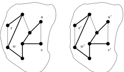
Let G = (V, E) be a graph (together with an assignment ID of vertex identifiers), T be a subgraph and let e1 = (u, v) and e2 = (z, w) be two of its edges. (See example in Figure 3.) Let
G0 = (V0, E0) be some copy of G = (V, E), where the identifiers of the vertices in V0 are not only pairwise distinct but also distinct from the given identifiers on V . Consider the following graphs G2 and GX and the subgraph T2.
• Graph G2 is simply G2 = (V2, E2) = G ∪ G0 = (V ∪ V0, E ∪ E0). The subgraph T2 of G2 is
defined as the union of the two copies of T , one in G and the other in G0. See example in Figure 4. Note that G2 is not connected, hence it is not a legal input to our problem.
• The graph GX is a “cross-wired” version of G2. Formally, GX = (V2, EX), where EX =
E2 r {(u, v), (z0, w0)} ∪ {(u, w0), (v, z0)}. (Observe that for e1, e2 ∈ T , T/ 2 is also a subgraph
of GX.) See example in Figure 5.
Let Π be a protocol that correctly solves the ST verification problem. Fix G to be some arbitrary graph, fix a copy G0 of G, fix a spanning tree T of G, and consider the execution of Π on either of the graphs G, G0, G2 and GX with the ST candidates T, T, T2 and T2, respectively. We stress that G2 (with candidate T2) is not a valid input for the ST (or the MST) verification problem since it is not connected. Still, we can consider the execution EX(Π, G2, T2), without requiring anything from its output.
Lemma 5.1 Let e1 ∈ E \ E(T ) and e02 ∈ E0\ E0(T ), such that no message is sent over the edges
e1 and e02 in execution EX(Π, G2, T2). Then executions EX(Π, G2, T2) and EX(Π, GX, T2) are
u v u’ v’ w z z’ w’
Figure 4: Graph G2 with ST candidate T2 (the bold edges belong to T2)
u v u’ v’ w z z’ w’
Figure 5: Graph GX with ST candidate T2 (the bold edges belong to T2)
Proof We show that in both executions each vertex sends and receives identical sequences of messages in each communication round of the protocol. Note that at each round the messages sent by some vertex x are dependent on x’s topological view (neighbors of x), x’s initial input (its identity and the indicator variables of the edges incident to x), and the set of messages sent and received by x in previous communication rounds. Denote by EX2 and EXX executions EX(Π, G2, T2) and EX(Π, GX, T2) respectively. Note that any vertex x ∈ V2r {u, v, z0, w0} has identical topological view and identical initial input in both executions. Vertex u has identical initial input and identical number of neighbors in both executions. Although the communication link connecting u to v in G2 connects u to w0 in GX, vertex u is initially unaware of this difference between the executions since it does not know the identifiers of its neighbors. (The same holds for vertices v, z0 and v0.) The proof is by induction on r, the number of communication rounds of protocol Π.
Induction base: For r = 0. In the first communication round, the messages sent by each vertex depend solely on its topological view and initial input. Let us analyze the sequence of messages sent by vertices in V (the vertices of graphs G2 and GX that belong to the first copy of G). Following are the possible cases.
• Vertex x /∈ {u, v}: Vertex x has identical topological view and identical initial input in both execution, thus it sends identical sequences of messages in the first round of both executions.
• Vertex u: As mentioned above, although in execution EXX vertex u is connected to w0instead
of v, it has no knowledge of this difference. Thus u sends identical sequences of messages over each of its communication links. The fact that no messages are sent over edge e in execution EX2, implies that in execution EXX no message is sent by u to its neighbor w0. Thus, u sends identical sequences of messages in the first communication round of both executions.
• Vertex v: can be analyzed in the same manner as vertex u.
The above shows that vertices in V send the same sequence of messages in the first communication round of both executions. The induction base claim follows by applying the same argument on vertices of V0.
Inductive step: Can be shown using a similar case analysis as in the induction base.
Theorem 1.2 follows as a consequence of the following Lemma. Lemma 5.2 Execution EX(Π, G2, T2) requires Ω(|E2r T2|) messages.
Proof Assume, towards contradiction, that there exists a protocol Π that correctly solves the ST verification problem for every graph G and ST candidate T , such that execution EX(Π, G, T ) sends fewer than |E r T |/2 messages over edges from E r T .
For the rest of the proof we fix G = (V, E) to be an arbitrary connected graph and denote the ST candidate by T . We take T to be a spanning tree and not just any subgraph. (See Figure 3).
Consider the graph G2 as previously defined with ST candidate T2 = {e = (x, y) ∈ T } ∪ {e0 = (x0, y0) | e = (x, y) ∈ T } (See Figure 4).
Then by the assumption on Π, execution EX2 = EX(Π, G2, T2) sends fewer than |E2r T2|/2 messages over edges from E2 r T2. Hence there exist e1 = (u, v) and e02 = (w0, z0) such that
e1, e02 ∈ E2r T2 and no message is sent over e1 and e02 in execution EX2. Consider the graph GX
with ST candidate T2 as previously defined (See Figure 5).
By Lemma 5.1, executions EX2 and EXX = EX(Π, GX, T2) are similar. Note that e1, e02 ∈ T/ 2,
thus T2 is not a spanning tree of GX (since the two copies of G contained in GX are connected solely by edges e1 and e02). Since Π correctly solves the ST verification problem, the output of all
vertices in EXX is “0” (i.e., the given ST candidate T2 is not a spanning tree of the graph GX). On the other hand, consider the execution EX = (Π, G, T ) with ST candidate T . Note that EX is exactly the restriction of EX2 on the first copy of G contained in G2. Since G2 contains two disconnected copies of G the output of all vertices in execution EX2 will be identical to the output of the same vertices in EX (since in both executions the vertices have identical topological view and the input variables contain identical values). Since executions EX2 and EXX are similar, the output of EX is “0”, in contradiction to the correctness of Π.
References
[1] Y. Afek, S. Kutten, and M. Yung. The local detection paradigm and its applications to self stabilization. Theoretical Computer Science, 186(1-2):199–230, 1997.
[2] B. Awerbuch. Optimal distributed algorithms for minimum weight spanning tree, counting, leader election, and related problems. In Proc. 19th ACM Symp. on Theory of computing (STOC), 230–240, NY, 1987.
[3] B. Awerbuch, B. Patt-Shamir, and G. Varghese. Self-stabilization by local checking and cor-rection. In Proc. IEEE Symp. on the Foundations of Computer Science, 268–277, 1991. [4] B. Awerbuch, O. Goldreich, R. Vainish, and D. Peleg. A trade-off between information and
communication in broadcast protocols. J. ACM, 37(2):238–256, 1990.
[5] A.L. Buchsbaum, L. Georgiadis, H. Kaplan, A. Rogers, R.E. Tarjan, and J.R. Westbrook. Linear-time algorithms for dominators and other path-evaluation problems. SIAM J. on Com-puting, 38(4):1533–1573, 2008.
[6] J.E. Burns. A formal model for message passing systems. Technical Report TR-91, Computer Science Dept., Indiana University, Bloomington, 1980.
[7] I. Cidon, I. Gopal, M. Kaplan, and S. Kutten. A distributed control architecture of high-speed networks. IEEE Trans. on Communications, 43(5):1950–1960, 1995.
[8] A. Das Sarma, S. Holzer, L. Kor, A. Korman, D. Nanongkai, G. Pandurangan, D. Peleg, and R. Wattenhofer. Distributed verification and hardness of distributed approximation. In Proc. 43th ACM Symp. on Theory of computing (STOC), 2011.
[9] A. Das Sarma, D. Nanongkai, and G. Pandurangan. A tight unconditional lower bound on distributed random walk computation. In Proc. 30th ACM SIGACT-SIGOPS Symp. on Prin-ciples of Distributed Computing (PODC), 2011.
[10] B. Dixon, M. Rauch, and R.E. Tarjan. Verification and sensitivity analysis of minimum span-ning trees in linear time. SIAM J. on Computing, 21(6):1184–1192, 1992.
[11] B. Dixon and R.E. Tarjan. Optimal parallel verification of minimum spanning trees in loga-rithmic time. Algologa-rithmica, 17(1):11–18, 1997.
[12] S. Dolev, M. Gouda, and M. Schneider. Requirements for silent stabilization. Acta Informatica, 36(6):447–462, 1999.
[13] P. Fraigniaud, A. Korman, and D. Peleg. Local Distributed Decision. FOCS 2011: 708-717 [14] P. Fraigniaud, A. Korman, M. Parter, and D. Peleg. Randomized Distributed Decision. DISC
2012: 371-385
[15] G.N. Frederickson and N.A. Lynch. The impact of synchronous communication on the problem of electing a leader in a ring. In Proc. 16th ACM Symp. on Theory of computing (STOC), 493–503, NY, 1984.
[16] M. L. Fredman and D. E. Willard. Trans-dichotomous algorithms for minimum spanning trees and shortest paths. Proc. 31st IEEE FOCS, 719–725, 1990.
[17] R. G. Gallager, P. A. Humblet, and P. M. Spira. A distributed algorithm for minimum-weight spanning trees. ACM Trans. Program. Lang. Syst., 5(1):66–77, 1983.
[18] J. Garay, S. A. Kutten, and D. Peleg. A sub-linear time distributed algorithm for minimum-weight spanning trees. SIAM J. on Computing, 27(1):302–316, 1998.
[19] R. L. Graham and P. Hell. On the history of the minimum spanning tree problem. Ann. Hist. Comput., 7(1):43–47, 1985.
[20] D. Harel. A linear time algorithm for finding dominators in flow graphs and related problems. In Proc. 17th ACM Symp. on Theory of computing (STOC), 185–194, 1985.
[21] D.R Karger, P.N. Klein, and R. E. Tarjan. A randomized linear-time algorithm to find mini-mum spanning trees. J. ACM, 42(2):321–328, 1995.
[22] M. Katz, N.A. Katz, A. Korman, and D. Peleg. Labeling schemes for flow and connectivity. SIAM J. Comput., 34(1):23–40, 2005.
[23] V. King. A simpler minimum spanning tree verification algorithm. Algorithmica, 18:263–270, 1997.
[24] V. King, C.K Poon, V Ramachandran, and S. Sinha. An optimal erew pram algorithm for minimum spanning tree verification. Information Processing Letters, 62(3):153–159, 1997. [25] J. Koml`os. Linear verification for spanning trees. Combinatorica, 5:57–65, 1985.
[26] A. Korman and S. Kutten. Distributed verification of minimum spanning trees. Distributed Computing, 20(4):253–266, 2007.
[27] A. Korman, S. Kutten, and D Peleg. Proof labeling schemes. Distributed Computing, 22(4):215–233, 2010.
[28] E. Kushilevitz and N. Nisan. Communication complexity. Cambridge Univ. Press, NY, 1997. [29] S. Kutten and D. Peleg. Fast distributed construction of small k-dominating sets and
appli-cations. J. Algorithms, 28(1):40–66, 1998.
[30] S. Kutten, G. Pandurangan, D. Peleg, P. Robinson, and A. Trehan. Universal Bounds for Leader Election. Unpublished manuscript, 2012.
[31] Z. Lotker, B. Patt-Shamir, and D. Peleg. Distributed mst for constant diameter graphs. In Proc. 20th ACM Symp. on Principles of distributed computing (PODC), 63–71, NY, 2001. [32] D. Peleg and V. Rubinovich. A near-tight lower bound on the time complexity of distributed
minimum-weight spanning tree construction. SIAM J. Comput., 30(5):1427–1442, 2000. [33] S. Pettie and V. Ramachandran. An optimal minimum spanning tree algorithm. J. ACM,
49(1):16–34, 2002.
[34] V. Rubinovich. Distributed minimum spanning tree construction. Master’s thesis, Department of Computer Science and Applied Mathematics, The Weizmann Institute of Science, 1999. [35] R.E. Tarjan. Applications of path compression on balanced trees. J. ACM, 26:690–715, 1979. [36] R.E. Tarjan. Data Structures and Network Algorithms. SIAM, 1983.