Comparing linear and neural models for competitive MWE identification

(1)

HAL Id: hal-02436433

https://hal.archives-ouvertes.fr/hal-02436433

Submitted on 13 Jan 2020

HAL is a multi-disciplinary open access archive for the deposit and dissemination of sci-entific research documents, whether they are pub-lished or not. The documents may come from teaching and research institutions in France or abroad, or from public or private research centers.

L’archive ouverte pluridisciplinaire HAL, est destinée au dépôt et à la diffusion de documents scientifiques de niveau recherche, publiés ou non, émanant des établissements d’enseignement et de recherche français ou étrangers, des laboratoires publics ou privés.

Comparing linear and neural models for competitive

MWE identification

Hazem Al Saied, Marie Candito, Mathieu Constant

To cite this version:

Hazem Al Saied, Marie Candito, Mathieu Constant. Comparing linear and neural models for com-petitive MWE identification. The 22nd Nordic Conference on Computational Linguistics, Sep 2019, Turku, Finland. �hal-02436433�

(2)

Comparing linear and neural models for competitive MWE identification

Hazem Al Saied ATILF, Universit´e de Lorraine

France halsaied@atilf.fr

Marie Candito LLF, Universit´e Paris Diderot

France

marie.candito@gmail.com

Mathieu Constant ATILF, Universit´e de Lorraine

France

mathieu.constant@univ-lorraine.fr

Abstract

In this paper, we compare the use of lin-ear versus neural classifiers in a greedy transition system for MWE identification. Both our linear and neural models achieve a new state-of-the-art on the PARSEME 1.1 shared task data sets, comprising 20 languages. Surprisingly, our best model is a simple feed-forward network with one hidden layer, although more sophisticated (recurrent) architectures were tested. The feedback from this study is that tuning a SVM is rather straightforward, whereas tuning our neural system revealed more challenging. Given the number of lan-guages and the variety of linguistic phe-nomena to handle for the MWE identifi-cation task, we have designed an accurate tuning procedure, and we show that hyper-parameters are better selected by using a majority-vote within random search figurations rather than a simple best con-figuration selection.

Although the performance is rather good (better than both the best shared task system and the average of the best per-language results), further work is needed to improve the generalization power, espe-cially on unseen MWEs.

1 Introduction

Multi-word expressions (MWE) are composed of several words (more precisely of elements that are words in some contexts) that exhibit irregularities at the morphological, syntactic and/or semantic level. For instance, ”prendre la porte” is a French verbal expression with semantic and morphological idiosyncrasy because (1) its idiomatic meaning (”to leave the room”) differs from its literal meaning (”to take the

door”) and (2) the idiomatic reading would be lost if ”la porte” were used in the plural. Identifying MWE is known to be challenging (Constant et al., 2017), due to the highly lexical nature of the MWE status, the various degrees of the MWE irregularities and the various linguistic levels in which these show. In this paper we focus on the task of identifying verbal MWEs, which have been the focus of two recent shared tasks, accompanied by data sets for 20 languages: PARSEME shared task ST.0 (Savary et al., 2017) and ST.1 (Ramisch et al., 2018). Verbal MWEs are rather rare (one every 4 sentences overall in ST1.1 data sets) but being predicates, they are crucial to downstream semantic tasks. They are unfortunately even more difficult to identify than other categories of MWEs: they are more likely to be discontinuous sequences and to exhibit morphological and structural variation, if only the verb generally shows full inflectional variation, allows adverbial modification and in some cases syntactic reordering such as relativization.

Our starting point to address the MWE iden-tification task is to reuse the system of Al Saied et al. (2018), an enhanced version of the winning system of ST.0, a transition system using a linear (SVM) model. Our objective has been to incor-porate neural methods, which are overwhelming in current NLP systems. Neural networks have brought substantial performance improvements on a large variety of NLP tasks including transition-based parsing (e.g. Kiperwasser and Goldberg (2016) or Andor et al. (2016)), in particular thanks to the use of distributed representations of atomic labels, their ability to capture contextual informa-tion. Moreover, neural methods supposedly learn combinations from simple feature templates, as an alternative to hand-crafted task-specific feature engineering.

(3)

Yet, using neural methods for our task is challenging, the sizes of the available corpus are relatively modest (no ST.1 language has more than 5000 instances of training MWEs), albeit neural models generally have more parameters to learn than linear models. Indeed, the best systems at the shared tasks ST.0 and ST.1 (Al Saied et al., 2017; Waszczuk, 2018) (in closed track) are not neural and surpassed some neural approaches.

In this paper, we carefully describe and com-pare the development and tuning of linear versus neural classifiers, to use in the transition system for MWE identification proposed in Al Saied et al. (2018), which itself built on the joint syntactic / MWE analyzer of Constant and Nivre (2016). We set ourselves the constraints (i) of building systems that are robust across languages, hence using the same hyperparameter configuration for all languages and (ii) of using lemma and POS information but not syntactic parses provided in the PARSEME data sets, so that the resulting systems require limited preprocessing. We report a systematic work on designing and tuning linear and neural transition classifiers, including the use of resampling, vocabulary generalization and several strategies for the selection of the best hyperparameter configuration. We address both the open and closed tracks of the PARSEME ST.1, i.e with and without external resources (which in our case amount to pre-trained word embeddings).

The contributions of our work are:

• a new state-of-the art for the MWE identifica-tion task on the PARSEME ST1.1 data sets. Our neural model obtains about a four-point error reduction on an artificial score mixing the best results for each language, and 4.5 points compared to the best participating sys-tem (even though we do not use syntactic parses);

• a report on which hyperparameters proved crucial to obtain good performance for the neural models, knowing that a basic feed-forward network without class balancing showed high instability and achieves very poorly (average F-score between 15% and 30%);

• an alternative strategy for tuning the hyperpa-rameters, based on trends in random search

(Bergstra and Bengio, 2012);

• a fine-grained analysis of the results for vari-ous partitions of the MWE, shedding light on the necessity to address unknown MWE (not seen in train);

• a negative result concerning the basic semi-supervised strategy of using pre-trained word embeddings.

We discuss the related work in Section 2, data sets in Section 3 and the transition system in Sec-tion 4. Linear and neural models are described in Sections 5 and 6, and the tuning methodology in Section 7. We present experiments and discuss results in Sections 8 and 9, and conclude in Sec-tion 10.

2 Related work

Supervised MWE identification has made sig-nificant progress in the last years thanks to the availability of new annotated resources (Schneider et al., 2016; Savary et al., 2017; Ramisch et al., 2018). Sequence tagging methods have been largely used for MWE identification. In particular, first studies experimented IOB or IOB-like anno-tated corpora to train conditional random fields (CRF) models (Blunsom and Baldwin, 2006; Constant and Sigogne, 2011; Vincze et al., 2011) or other linear models (Schneider et al., 2014).

Recently, Gharbieh et al. (2017) experimented on the DiMSUM data set various IOB-based MWE taggers relying on different deep learning models, namely multilayer perceptron, recurrent neural networks and convolutional networks. They showed that convolutional networks achieve better results. On the other hand, Taslimipoor and Rohanian (2018) used pre-trained non-modifiable word embeddings, POS tags and other technical features to feed two convolutional layers with window sizes 2 and 3 in order to detect n-grams. The concatenation of the two layers is then passed to a Bi-LSTM layer.

Legrand and Collobert (2016) used a phrase representation concatenating word embeddings in a fixed-size window, combined with a linear layer in order to detect contiguous MWEs. They reach state-of-the-art results on the French Treebank (Abeill´e et al., 2003; Seddah et al., 2013). Ro-hanian et al. (2019) integrate an attention-based

(4)

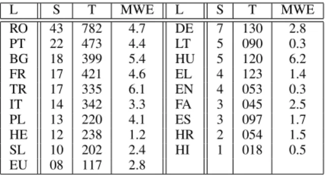
L S T MWE L S T MWE RO 43 782 4.7 DE 7 130 2.8 PT 22 473 4.4 LT 5 090 0.3 BG 18 399 5.4 HU 5 120 6.2 FR 17 421 4.6 EL 4 123 1.4 TR 17 335 6.1 EN 4 053 0.3 IT 14 342 3.3 FA 3 045 2.5 PL 13 220 4.1 ES 3 097 1.7 HE 12 238 1.2 HR 2 054 1.5 SL 10 202 2.4 HI 1 018 0.5 EU 08 117 2.8

Table 1: The number of Sentences, Tokens and MWEs in train sets of ST.1 Languages. Dev and test sets have all a close number of MWEs (between 500 and 800). Languages are represented by their ISO 639-1 code and all table numbers are scaled and rounded (1/1000).

neural model with a graph convolutional neural network to produce an efficient model that outper-forms the state-of-the-art on certain languages of the PARSEME Shared Task 1.1.

The work of Waszczuk (2018) extends a se-quential CRF to tree structures, provided that MWEs form connected syntactic components and that dependency parse trees are given as input. De-pendency trees are used to generate a hypergraph of possible traversals and a binary classifier labels nodes as MWEs or not using local context infor-mation. A multi-class logistic regression is then used to determine the globally optimal traversal. This method has showed very competitive scores on the data sets of the PARSEME ST1.1, by rank-ing first overall on the closed track.

By contrast, some authors have used Transition systems, introducing a greedy structured method that decomposes the MWE prediction problem into a sequence of local transition predictions. Constant and Nivre (2016) proposed a two-stack transition system to jointly perform MWE iden-tification and syntactic parsing. Al Saied et al. (2017) experimented a partial implementation of this system for identifying and categorizing ver-bal MWEs. This system eliminates the syntac-tic aspects of Constant and Nivre (2016)’s system and learn a SVM model using linguistic and tech-nical features to classify transitions. Relying on Al Saied et al. (2017), Stodden et al. (2018) re-placed the linear model with a convolutional mod-ule that transforms the sparse feature vectors into continuous ones and connect them to a dense layer.

Name Cond. Action

Figure 1:Set of transitions, each with its precondition.

3 Data sets

For our investigation, we focus on the data sets of the PARSEME Shared Task on verbal MWE iden-tification edition 1.1 (Ramisch et al., 2018), there-after ST.1. Table 1 provides statistics on this data set, which includes 20 languages1covering a wide range of families and corpus sizes. All languages come with train and test sets, and all but EN, HI and LT have a development set. They contain tok-enized sentences in which MWEs are annotated. Each token comes with its word and lemma forms and its part of speech (POS) tag. ST.1 also has extra linguistic annotations such as morphologi-cal features and syntactic dependency trees, but we do not use them for the purpose of the pa-per. One MWE instance is either a set of sev-eral potentially non-continuous tokens, or a sin-gle token compounding multiple words (namely a multiword token, hereafter MWT).2Data sets also contain rare MWEs embedded in another one, and overlapping MWEs.

4 System description

Transition system A transition system incre-mentally builds the expected output structure by sequentially applying a transition to a con-figuration that encodes the state of the system, outputting a new configuration. It has been used in particular to build a syntactic tree for a given input sentence (Nivre, 2004), and to build both the syntactic tree and the MWE list (Constant and Nivre, 2016). We use such a system here to build the list of MWEs only.We reuse the transition system of Al Saied et al. (2018), simplified in that we do not predict the MWE types.

In this system, a configuration is a triplet c = (σ, β, γ), where β is a buffer of (remaining) tokens, σ is a stack of ”elements”, which are either single tokens or binary trees of tokens, and γ is the list of elements that have been

1

We used all languages but Arabic due to licence issues.

2_{MWTs are extremely marginal for all ST.1 languages}

(5)

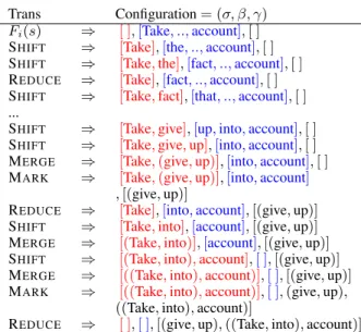
Trans Configuration = (σ, β, γ) Fi(s) ⇒ [ ],[Take, .., account], [ ]

SHIFT ⇒ [Take],[the, .., account], [ ] SHIFT ⇒ [Take, the],[fact, .., account], [ ] REDUCE ⇒ [Take],[fact, .., account], [ ] SHIFT ⇒ [Take, fact],[that, .., account], [ ] ...

SHIFT ⇒ [Take, give],[up, into, account], [ ] SHIFT ⇒ [Take, give, up],[into, account], [ ]

MERGE ⇒ [Take, (give, up)],[into, account], [ ] MARK ⇒ [Take, (give, up)],[into, account]

, [(give, up)]

REDUCE ⇒ [Take],[into, account], [(give, up)] SHIFT ⇒ [Take, into],[account], [(give, up)] MERGE ⇒ [(Take, into)],[account], [(give, up)] SHIFT ⇒ [(Take, into), account],[ ], [(give, up)] MERGE ⇒ [((Take, into), account)],[ ], [(give, up)] MARK ⇒ [((Take, into), account)],[ ], (give, up),

((Take, into), account)]

REDUCE ⇒ [ ],[ ], [(give, up), ((Take, into), account)] Figure 2: Application of the oracle transition sequence for the sentence Take the fact that I didn’t give up into account, containing two verbal MWEs: Take into account and give up.

identified as MWEs so far3. To build the list of MWEs for a given input sentence w1, w2, ...wn,

the system starts by the initial configuration (σ = [ ], β = [w1, ..., wn], γ = [ ]), and applies

a sequence of transitions until a terminal config-uration is reached, namely here when both the buffer and stack are empty. The transition set, and their precondition is described in Figure 1. Note the MERGEtransition creates complex stack elements, by merging the top 2 elements of the stack4.

The identification of a MWE made of m com-ponents t1, ..., tm necessitates m − 1 MERGEs,

and one final MARK. The REDUCE transition allows to manage discontinuities in MWEs. Note that MARK identifies S0 as MWE, but does

not remove it from the stack, hence enabling to identify some cases of embedded MWEs (we refer to Al Saied et al. (2018) for the precise expressive power). At prediction time, we use a greedy algorithm in which the highest-scoring applicable transition according to a classifier is applied to the current configuration.

Learning algorithm and oracle To learn this

3_{In all the following, we use σ|i to denote a stack with}

top element i and remainder σ, and i|β for a buffer with first token i followed by the elements in β. Siand Bidenote the

ith element of the stack and buffer respectively, starting at 0.

4_{Hence S}

i elements are either single tokens or binary

trees of tokens. In the latter case, their linguistic attributes (lemma, POS, word form) are obtained by simple concatena-tion over their components.

Tuning BoR TB Feature template Prelim + + Unigrams S0, S1, B0

Prelim + + Bigrams S0S1, S0B0, S0B1, S1B0

Prelim + + Lemma ngrams and POS ngrams

Prelim + + S0in MWT dictionary

Prelim - - Resampling

Rdm Sch - - word forms ngrams

Rdm Sch + - Unigram B1

Rdm Sch + - Bigram S0B2

Rdm Sch + - Trigram S1S0B0

Rdm Sch + + Distance between S0and S1

Rdm Sch + + Distance between S0and B0

Rdm Sch + - MWE component dictionary Rdm Sch - - Stack length

Rdm Sch + + Transition history (length 1) Rdm Sch - + Transition history (length 2) Rdm Sch + - Transition history (length 3)

FG 62.5 60

Table 2: Linear model feature hyperparameters. First col-umn: prelim if the hyperparameter was fixed once and for all given preliminary tests vs. Rdm Sch for tuning via random search (see Section 7). Best of random BoR column: whether the template is activated (+) or not (-) in the best performing hyperparameter set of the random search. Trend-based TB: same but for the trend-based hyperparameter set (cf. sec-tion 7). The last line provides the corresponding global F-scores on dev sets of the three pilot languages (BG, PT and TR).

transition classifier, we use the static deterministic oracle of Al Saied et al. (2018). For any input sentence and list of gold MWEs, the oracle defines a unique sequence of transitions, pro-viding example pairs (config / next transition to apply). Transitions have a priority order (MARK > MERGE> REDUCE> SHIFT), and the oracle greedily applies the highest-priority transition that is compatible with the gold analysis. MERGE is gold-compatible whenever S0 and S1 are part

of the same gold MWE.5 For REDUCE to be gold-compatible, S0 must not be strictly included

in a gold MWE. Moreover, either S0 is not a gold

MWE, or it is already marked as MWE.

Figure 2 shows the application of the ora-cle transition sequence for a sentence with two MWEs.6

5 Linear model

In order to compare linear and neural models for MWE identification, we reused the best

5_{Note that this order will lead to left-branching binary}

trees for elements in the stack.

6

The system is implemented in Python 2.7, using Keras and Scikit-learn libraries. The code is available

at https://github.com/hazemalsaied/MWE.

Identification/releases/tag/v.1 under MIT

(6)

performing linear model of Al Saied et al. (2018), namely a SVM, in a one versus rest scheme with linear kernel and squared hinge loss.

We used the feature templates of Al Saied et al. (2018) minus the syntactic features, since we focus on MWE identification independently of syntactic parsing. Table 2 displays the list of feature templates. We detail the ”S0 in MWT

dictionary” and ”MWE component dictionary” templates, the other features names being rather transparent: ”S0in MWT dictionary” feature fires

when S0 lemma is a MWT at least once in train,

and binary features fire when either S0, S1, B0,

B1 or B2 belong to at least one train multi-token

MWE.

We ran some preliminary experiments which led us to set some hyperparameters once and for all (first four lines of Table 2). In particular, we ended up not using resampling to balance the class distri-bution, because it proved quite detrimental for the linear model, contrary to the neural models. We then performed tuning for all the other features (cf. section 7).

6 MLP model

Though we investigated various neural archi-tectures7, the ”baseline” multi-layer perceptron (hereafter MLP) proved to be the best in the end. It is a plain feed-forward network, with an embedding layer concatenating the embeddings for the POS of S0, S1, B0 and B1 and for either

their word form or lemma (hyperparameter), fully connected to a dense layer with ReLU activation, in turn connected to the output layer with softmax activation.

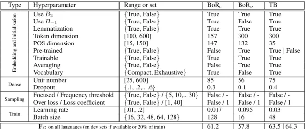
Table 3 provides the exhaustive list of MLP hyperparameters, along with their possible values and their optimal values for the most performing

7

We tried in particular (1) a MLP with several hidden lay-ers; (2) a MLP fed with a bidirectional recurrent layer to rep-resent the sequence of elements S0S1B0; (3) We also built a

model inspired by Kiperwasser and Goldberg (2016) in which the recurrent (LSTM) embeddings of certain focus elements (S0, S1, B0 and B1) are dynamically concatenated and fed

into a MLP, with back-propagation for a whole sentence in-stead of for each transition. The recurrent representations of the focus elements are supposed to encode the relevant con-textual information of these elements in the sentence. These models suffered from either a non-competitive performance or a very unstable loss (36.7 for the bidirectional MLP and 8.4 for kiperwasser on test data sets of ST1.1).

configurations. Lines 1 to 9 correspond to embed-ding and initialization hyperparameters: Lines (1, 2) concern which elements to include as additional input (Use B2, Use B−1)8, (3) which form for

input tokens (Lemmatization), (4, 5) which size for token and POS tag embeddings (Token and POS dimensions), (6) whether the embeddings are initialized randomly or pre-trained (pre-trained), (7) whether the embeddings are Trainable or not, and (8) how to generate embedding vectors for stack elements: as the average of tree token embeddings or as their sum (Averaging).

Vocabulary For the neural model, when Si

or Bi are missing, a special dummy word is used

instead. Moreover, we investigated an aggressive reduction of the known vocabulary. We compared 2 strategies to define it: in exhaustive vocabulary mode, hapaxes are replaced at training time by a UNK symbol, with probability 0.5. In compact vocabularymode, any token (or complex element) whose lemma is never a component of a MWE in the training set is replaced by UNK. Note that in both modes, the used vocabulary contains the con-catenated symbols in case of complex Sielements.

Resampling Given that tokens are mostly not part of a VMWE, the transitions for their identi-fication are very rare, leading to a very skewed class distribution.9Resampling techniques aiming at balancing class distribution are known to be efficient in such a case (Chawla, 2009). Moreover, preliminary experiments without resampling showed unstable loss and rather low performance. We thus used in subsequent experiments a hy-brid resampling method composed of (1) under sampling, that removes training sentences non containing any MWE, and (2) random over-sampling, that forces a uniform distribution of the classes by randomly duplicating minority class instances (all but SHIFT) (Chawla, 2009). Preliminary experiments showed that without these strategies, the systems suffered from very unstable loss and low performance, which led us to systematically use these two strategies in the subsequent experiments.

8_B

−1is the last reduced element (its right-most token if

it is a complex stack element).

9_{For all ST.1 languages, the transitions in training sets are}

approximately distributed as follows: 49% for SHIFT, 47% for REDUCE, 3% for MERGEand 1% for MARK.

(7)

Type Hyperparameter Range or set BoRc BoRo TB

Embedding

and

initialisation

Use B2 {True, False} True True True

Use B−1 {True, False} True False True

Lemmatization {True, False} True True True

Token dimension [100, 600] 157 300 300

POS dimension [15, 150] 147 132 35

Pre-trained {True, False} False True True | False

Trainable {True, False} True True True

Averaging {True, False} False True True

Vocabulary {Compact, Exhaustive} True False True

Dense Unit number [25, 600] 85 56 75

Dropout {.1, .2,.. .6} 0.3 0.1 0.4

Sampling Focused / Frequency threshold {True, False} / {5, 10,.. 30} False / - False / - False /

-Over loss / Loss coefficient {True, False} / [1, 40] False / 1 False / 1 False / 1

Train Learning rate [.01, .2] 0.017 0.095 0.03

Batch size {16, 32, 48, 64, 128} 128 16 48

FGon all languages (on dev sets if available or 20% of train) 61.2 57.8 63.5 | 64.3

Table 3: MLP hyperparameters and their possible values (”range or set” column). Best-of-random closed (BoRc) and

Best-of-random open (BoRo) columns: hyperparameter values in best configurations according to random search on the three pilot

languages, in closed and open tracks. Last column: Trend-based (TB) configuration (see text in section 7). Last line: global F-scores for these configurations, calculated using the average precision and recall for all ST.1 languages. The models are fit on truncated training sets of the three pilot languages (BG, PT and TR) (cf. section 7).

Tuning explored two supplementary resampling techniques: ”focused” oversampling which aims at mimicking a minimum number of occurrences for all MWEs. When set, training instances with MERGEand MARK transitions are duplicated for each training MWE below a frequency threshold. ”Over loss” hyperparameter penalizes the model when it fails to predict MERGE and MARK, by multiplying the loss by a coefficient (see Table 3).

7 Tuning methodology

The tuning phase served us to choose a hyperpa-rameter configuration for the linear model and the neural model, in closed and open track. In our case, we experimented open track for the neural model only, by using pre-trained embeddings instead of random initialization. We thus consider three cases: closed track linear, closed track MLP and open track MLP.

For each of these three cases, in order to enforce the robustness across languages of the selected perparameters, we aimed at selecting the same hy-perparameter configuration for all the languages.

Yet, to reduce the tuning time, we have chosen to work on three pilot languages, from three different language families. But because the various training sets have various sizes, we tried to neutralize this variation by using training sets of average size. This led us to choose three languages (Bulgarian, Portuguese and Turkish) among ST.1 languages having training sets bigger

than average and to tune the hyperparameters using training sets truncated to that average size (270k tokens) and evaluating on dev sets.

Multilingual metric: the official metric for the PARSEME shared task is the macro average of the F-scores over all languages (hereafter FAV G).

Yet we noted that although macro-averaging precision and recall is appropriate because the number of dev and test MWEs is almost the same for all languages, averaging the F-scores of all languages sometimes substantially differs (e.g. by 2 points) from taking the F-score of the macro-averaged precision and the macro-averaged recall (hereafter FG). We thus use FAV G for

comparability with the shared task results, but also report the FGscore, and use the latter during

tuning.

Random search: To tune the hyperparame-ters on the three pilot languages, we used random search, which proved to be more efficient than grid search when using the same computational budget, because it allows to search larger ranges of values (Bergstra and Bengio, 2012). We thus run about 1000 trials for SVM, closed track MLP and open track MLP. For the SVM, random search used a uniform distribution for the hyperparam-eters, which are all boolean. For the MLP, the random hyperparameter values are generated from either a set of discrete values using a uniform distribution or from a range of continuous values

(8)

using logarithmic distribution. For the MLP, each resulting random hyperparameter configuration was run on each pilot language twice, using always the same two seeds 0 and 110. We then averaged the precision and recall on the dev sets, for the three languages and the two seeds (i.e. use the global F-score FG).

Selecting hyperparameter configurations: Random hyperparameter search for the three pilot languages led us to use two strategies to select the hyperparameter sets. The first one is simply to select the best performing hyperparameter sets (shown in column BoR in Table 2 for the linear model, and in the BoRcand BoRocolumns in

Ta-ble 3). Yet, we noted that some hyperparameters varied a lot among the top performing systems. We thus investigated to build a ”trend-based” configuration, by selecting each hyperparameter value according to the observed trend among the top k best configurations (with k=500/250 for MLP/SVM)11. This results in two sets for the linear model (best-of-random and trend-based, in closed mode) and four configurations for the MLP: best-of-random or trend-based, in closed or open mode.

We then trained these six configurations on the full-size training sets for all ST.1.1 languages, using two seeds (0 and 1), and retaining the best seed for each language. For the MLP case, the global F-scores on dev sets are provided in the last row of Table 3. Interestingly, the trend-based configuration largely beats the best-of-random configurations, both in closed and open tracks12. This shows that choosing hyperparameter values independently of each other is compensated by choosing more robust values, by using the top k best performing systems instead of one.

Note that for the linear case, the trend-based configuration does not surpass the best perform-ing random search configuration (the last line of

10

Preliminary experiments showed a relative stability when changing seeds, hence we used only two seeds in the end. Changing seeds was useless for the linear model which is more stable.

11_{We chose the values using an approximate majority vote,}

using a graphical visualization of the hyperparameter values in the top k best performing systems.

12_Moreover, _the _{best-of-random} _open _{configuration}

showed instability when switching from the three pilot lan-guages to all lanlan-guages, leading to a null score for Hindi (hence the rather low global F-score of 57.8).

Language Closed track Open track

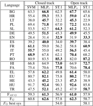
SVM MLPc ST.1 MLPo ST.1 BG 63.3 66.8 62.5 67.7 65.6 HR 55.4 59.3 55.3 59.0 47.8 LT 38.0 45.7 32.2 45.3 22.9 PL 69.4 71.8 67.0 72.2 63.6 SL 53.5 62.7 64.3 61.2 52.3 DE 49.5 51.5 45.3 49.9 45.5 EN 28.4 31.4 32.9 31.9 33.3 ES 39.2 40.0 34.0 39.7 38.4 FR 61.1 59.0 56.2 58.8 60.9 IT 55.7 55.0 49.2 56.5 45.4 PT 68.9 67.8 62.1 70.4 68.2 RO 80.9 83.5 85.3 82.0 87.2 HI 66.8 64.9 73.0 64.9 72.7 FA 75.4 70.6 77.8 70.6 78.4 EL 57.8 62.2 49.8 61.4 58.0 EU 80.7 82.1 75.8 80.2 77.0 HE 43.3 45.2 23.3 47.3 38.9 HU 91.7 92.4 90.3 92.6 85.8 TR 47.5 52.1 45.2 47.9 58.7 FAV G 59.3 61.3 56.9 61.0 57.9 FG 60.8 62.6 57.8 62.3 58.7 FGbest sys 54.0 58.1

Table 4: MWE-based F-scores for ST.1 languages on test sets using our tuned SVM and MLP models, fit on train and dev sets when available. ST.1 stands for the most perform-ing scores of the shared task for each language in closed and open tracks. All ST.1 systems fit training and development sets except the system that produced the best score of BG on closed track. Languages are grouped according to their linguistic families (Slavic, Germanic, Romance, Indo-Iranian and other).) FAV Gis the official metric (average F-scores).

FGis the global F-score (see Section 7). In the FAV Gand

FGlines, the best ST.1 per-language scores are used, whereas

the last line concerns the FGscore of the best ST.1 systems

(Waszczuk, 2018; Taslimipoor and Rohanian, 2018).

Table 2). This asymmetry could mean that the number of random trials is sufficient for the lin-ear case, but not for the neural models, and that a trend-based strategy is advantageous within a lim-ited computational budget.

8 Experiments and results

Table 4 provides identification scores on test sets, for our tuned SVM and MLP models for each ST.1 language, along with the best score of ST.1 for each language, in open and closed tracks. It also displays overall scores using both the official ST.1 metrics (FAV G) and the more precise FG

score introduced in section 7. This FG score for

the ST.1 results is computed in two modes: in line FG, the ST.1 columns correspond to artificially

averaging the best result of each language (in closed / open tracks), whereas ”FGbest sys” is the

score of the best system of ST.1. The differences between SVM and MLPc results are significant13

(9)

for all languages except EU, HU, LT and PL. For both FAV G and FG metrics, results show

that MLP models significantly outperforms all other systems both in the closed and open tracks. In the closed track, MLP surpasses SVM by 1.8 points, the best ST.1 systems per language by 4.8 points, and the best ST.1 system (Waszczuk, 2018) by 8.6 points. In the open track, MLP beats the best ST.1 system (Taslimipoor and Rohanian, 2018) by 4.2 points, and the best ST.1 systems per language by 3.6 points14.

In the closed track, MLP ranks first for 11 languages, while the SVM model and the best ST.1 systems per language reach the first position respectively for three and five languages. In open track, MLP achieves the highest scores for 13 languages while ST.1 systems beat it for six languages. These results tend to validate the robustness of our approach across languages. Regarding language families, MLP reports remarkable gains for Slavic languages and lan-guages from the other family, but achieve lower performance on Indo-Iranian languages when compared with best ST.1 results. For Romance languages, our models surpass the ST.1 best results (except for RO), and the SVM model is globally better than the MLP.

Comparing the results of the open and the closed track, we can observe that the use of pre-trained word embeddings has no significant im-pact on the MLP results. This might mean that static embeddings are not well-suited for repre-senting tokens both when used literally and within MWE. This tendency would deserve more investi-gation using other word embedding types, in par-ticular contextualized ones (Devlin et al., 2018).

9 Discussion

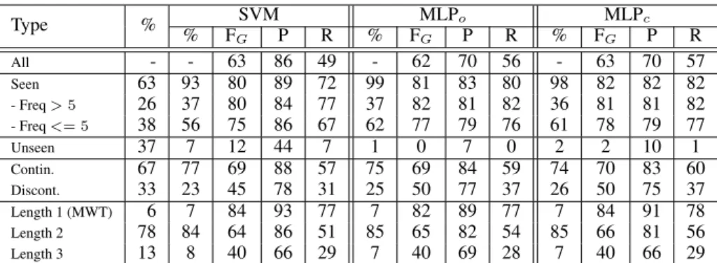
Performance analysis In order to better under-stand the strengths and weaknesses of the various systems, we provide in Table 5 an in-depth performance analysis of our models, on dev sets, broken-down by various classifications of MWEs,

14

It is worth noting that the model of Rohanian et al. (2019), published while writing this paper, outperforms our scores for the languages they use for evaluating their model (EN:41.9, DE:59.3, FR:71.0, FA:80.0) on the ST.1 test sets. However, this model exploits syntactic information (See Sec-tion 2).

namely (1) whether a dev MWE was seen in train (and if so, more than 5 times or not) or unseen; (2) whether the MWE is continuous or has gaps; and (3) according to the MWE length. The table provides the proportions of each subclass within the gold dev set and within the predictions of each model (% columns), in addition to the average precision and recall over all languages, and the global FGscore, for each model. Overall,

neural models (in closed and open tracks) tends to get better recall than the SVM model (56 and 57, versus 49) but lower precision (70 versus 86), which is coherent with the use of embeddings. Generalization power Without surprise, the global F-score on seen MWEs is high for all our systems (> 80), and it is still above 75 for MWEs with frequency ≤ 5. Yet this masks that the neural models have comparable precision and recall on seen MWEs, whereas the SVM has better precision than recall. Now when turning to the unseen category, we can observe that all systems get very low performance.

In comparison with MLP models, the most important advantage of SVM is its (little) ability to generalize (FG = 12 on unseen MWEs),

whereas the MLPs have none at all. Note that frequency ≤ 5 is sufficient for the MLP models to surpass the linear model. For comparison, the average F-scores on test sets of the PARSEME ST.1 for unseen MWEs range from 0 to almost 20. This very low generalization of our MLP models is understandable since tuning led us to favor the compact vocabulary mode, which agressively reduces the known vocabulary to seen MWE components. Yet our best result on unseen MWEs with a MLP with exhaustive vocabulary mode only achieves FG = 4 on unseen MWEs.

It appears that for all models, more than 90% of the unindentified MWEs (the silence) are either unseen or with frequency ≤ 5, which clearly shows that the frequency of a MWE in train set is the crucial trait for identification. Further analysis is needed to study the performance according to the literal versus MWE ambiguity rate.

Continuous/discontinuous MWEs MLP

models show better performances for discon-tinuous MWEs than SVM, whereas they reach

(10)

Type % SVM MLPo MLPc % FG P R % FG P R % FG P R All - - 63 86 49 - 62 70 56 - 63 70 57 Seen 63 93 80 89 72 99 81 83 80 98 82 82 82 - Freq > 5 26 37 80 84 77 37 82 81 82 36 81 81 82 - Freq <= 5 38 56 75 86 67 62 77 79 76 61 78 79 77 Unseen 37 7 12 44 7 1 0 7 0 2 2 10 1 Contin. 67 77 69 88 57 75 69 84 59 74 70 83 60 Discont. 33 23 45 78 31 25 50 77 37 26 50 75 37 Length 1 (MWT) 6 7 84 93 77 7 82 89 77 7 84 91 78 Length 2 78 84 64 86 51 85 65 82 54 85 66 81 56 Length 3 13 8 40 66 29 7 40 69 28 7 40 66 29

Table 5: Performance of our tuned models, on all languages, with models fit on train and evaluated on dev sets if available, otherwise fit on 80% of train and evaluated on the rest (with seed 0 for MLP models). First line: performance on all languages. Subsequent lines: break-down according to various MWE classifications (first column). Second column: proportion of the subclass in gold dev set. For each model (SVM, MLPo(open)and MLPc(losed)), we report for each subclass: the proportion of

the subclass in the system prediction, the global F-score (FG), Precision (P) and Recall (R).

comparable scores for continuous MWEs. In particular, they display a 5-point gain in F-score, due to a 6-point gain in recall on discontinuous MWEs.

MWE length The three systems display com-parable scores regarding MWE length. Results validate the intuition that the shorter the MWE, the easier it is to identify.

10 Conclusion

We described and compared the development of linear versus neural classifiers to use in a transition system for MWE identification (Al Saied et al., 2018). Surprisingly, our best neural architecture is a simple feed-forward network with one hidden layer, although more sophisticated architectures were tested. We achieve a new state-of-the art on the PARSEME 1.1 shared task data sets, comprising 20 languages.

Our neural and linear models surpass both the best shared task system (Waszczuk, 2018) and the artificial average of the best per-language results. Given the number of languages and the variety of linguistic phenomena to handle, we designed a precise tuning methodology.

Our feedback is that the development of the linear (SVM) system was pretty straightforward, with low variance between the configurations. For the neural models on the contrary, preliminary runs led to low and unstable performance. Class balancing proved crucial, and our proposal to select hyperparameter values using majority vote on the top k best performing systems in random search also proved beneficial.

Although our systems are competitive, their generalization power reveals disappointing: per-formance on unseen MWEs is very low for the linear model (F-score=12) and almost zero for the neural models (whereas the shared task results range from 0 to 20 for unseen MWEs). Basic semi-supervised experiments, consisting in using pre-trained word embeddings, did not bring any improvement. Static embeddings might not be suitable representations of MWE components, as their behavior differs when used literally or within a MWE. This definitely calls for future work that can incorporate information on semantic irregular-ity.

Acknowledgement

This work was partially funded by the French Na-tional Research Agency (PARSEME-FR ANR-14-CERA-0001).

(11)

References

Anne Abeillé, Lionel Clément, and François Toussenel. 2003. Building a treebank for French. In Anne Abeillé, editor, Treebanks. Kluwer, Dordrecht. Hazem Al Saied, Marie Candito, and Matthieu

Con-stant. 2017. The ATILF-LLF system for parseme shared task: a transition-based verbal multiword ex-pression tagger. In Proceedings of the 13th Work-shop on Multiword Expressions (MWE 2017), pages 127–132, Valencia, Spain. Association for Compu-tational Linguistics.

Hazem Al Saied, Marie Candito, and Matthieu Con-stant. 2018. A transition-based verbal multiword expression analyzer. In Multiword expressions at length and in depth: Extended papers from the MWE 2017 workshop, volume 2, page 209. Language Sci-ence Press.

Daniel Andor, Chris Alberti, David Weiss, Aliaksei Severyn, Alessandro Presta, Kuzman Ganchev, Slav Petrov, and Michael Collins. 2016. Globally nor-malized transition-based neural networks. arXiv preprint arXiv:1603.06042.

James Bergstra and Yoshua Bengio. 2012. Random search for hyper-parameter optimization. Journal of Machine Learning Research, 13(Feb):281–305. Phil Blunsom and Timothy Baldwin. 2006.

Multilin-gual deep lexical acquisition for hpsgs via supertag-ging. In Proceedings of the 2006 Conference on Empirical Methods in Natural Language Process-ing, pages 164–171, Sydney, Australia. Association for Computational Linguistics.

Nitesh V Chawla. 2009. Data mining for imbalanced datasets: An overview. In Data mining and knowl-edge discovery handbook, pages 875–886. Springer. Mathieu Constant, G¨uls¸en Eryi˘git, Johanna Monti, Lonneke Van Der Plas, Carlos Ramisch, Michael Rosner, and Amalia Todirascu. 2017. Multiword ex-pression processing: A survey. Computational Lin-guistics, 43(4):837–892.

Matthieu Constant and Joakim Nivre. 2016. A transition-based system for joint lexical and syn-tactic analysis. In Proceedings of the 54th An-nual Meeting of the Association for Computational Linguistics (Volume 1: Long Papers), pages 161– 171, Berlin, Germany. Association for Computa-tional Linguistics.

Matthieu Constant and Anthony Sigogne. 2011. Mwu-aware part-of-speech tagging with a crf model and lexical resources. In Proceedings of the Workshop on Multiword Expressions: from Parsing and Gen-eration to the Real World, pages 49–56. Association for Computational Linguistics.

Jacob Devlin, Ming-Wei Chang, Kenton Lee, and Kristina Toutanova. 2018. BERT: pre-training of deep bidirectional transformers for language under-standing. CoRR, abs/1810.04805.

Waseem Gharbieh, Virendrakumar Bhavsar, and Paul Cook. 2017. Deep learning models for multiword expression identification. In Proceedings of the 6th Joint Conference on Lexical and Computational Semantics (*SEM 2017), pages 54–64, Vancouver, Canada. Association for Computational Linguistics. Eliyahu Kiperwasser and Yoav Goldberg. 2016. Sim-ple and accurate dependency parsing using bidirec-tional lstm feature representations. arXiv preprint arXiv:1603.04351.

Jo¨el Legrand and Ronan Collobert. 2016. Phrase rep-resentations for multiword expressions. In Proceed-ings of the 12th Workshop on Multiword Expres-sions, pages 67–71, Berlin, Germany. Association for Computational Linguistics.

Joakim Nivre. 2004. Incrementality in determinis-tic dependency parsing. In Proceedings of the ACL Workshop Incremental Parsing: Bringing En-gineering and Cognition Together, pages 50–57, Barcelona, Spain. Association for Computational Linguistics.

Carlos Ramisch, Silvio Cordeiro, Agata Savary, Veronika Vincze, Verginica Mititelu, Archna Bhatia, Maja Buljan, Marie Candito, Polona Gantar, Voula Giouli, et al. 2018. Edition 1.1 of the parseme shared task on automatic identification of verbal multiword expressions. In the Joint Workshop on Linguistic Annotation, Multiword Expressions and Constructions (LAW-MWE-CxG-2018), pages 222– 240.

Omid Rohanian, Shiva Taslimipoor, Samaneh Kouchaki, Le An Ha, and Ruslan Mitkov. 2019. Bridging the gap: Attending to discontinuity in identification of multiword expressions. arXiv preprint arXiv:1902.10667.

Agata Savary, Carlos Ramisch, Silvio Cordeiro, Fed-erico Sangati, Veronika Vincze, Behrang Qasem-iZadeh, Marie Candito, Fabienne Cap, Voula Giouli, and Ivelina Stoyanova. 2017. The parseme shared task on automatic identification of verbal multiword expressions.

Nathan Schneider, Emily Danchik, Chris Dyer, and Noah A. Smith. 2014. Discriminative lexical se-mantic segmentation with gaps: running the MWE gamut. TACL, 2:193–206.

Nathan Schneider, Dirk Hovy, Anders Johannsen, and Marine Carpuat. 2016. Semeval-2016 task 10: De-tecting minimal semantic units and their meanings (dimsum). In Proceedings of the 10th International Workshop on Semantic Evaluation (SemEval-2016), pages 546–559.

Djamé Seddah, Reut Tsarfaty, Sandra Kübler, Marie Candito, Jinho D. Choi, Richárd Farkas, Jen-nifer Foster, Iakes Goenaga, Koldo Gojenola Gal-letebeitia, Yoav Goldberg, Spence Green, Nizar Habash, Marco Kuhlmann, Wolfgang Maier, Joakim

(12)

Nivre, Adam Przepiórkowski, Ryan Roth, Wolfgang Seeker, Yannick Versley, Veronika Vincze, Marcin Woliński, Alina Wróblewska, and Eric Villemonte de la Clergerie. 2013. Overview of the SPMRL 2013 shared task: A cross-framework evaluation of pars-ing morphologically rich languages. In Proceed-ings of the Fourth Workshop on Statistical Parsing of Morphologically-Rich Languages, pages 146–182, Seattle, Washington, USA. Association for Compu-tational Linguistics.

Regina Stodden, Behrang QasemiZadeh, and Laura Kallmeyer. 2018. Trapacc and trapaccs at parseme shared task 2018: Neural transition tagging of ver-bal multiword expressions. In Proceedings of the Joint Workshop on Linguistic Annotation, Multi-word Expressions and Constructions (LAW-MWE-CxG-2018), pages 268–274.

Shiva Taslimipoor and Omid Rohanian. 2018. Shoma at parseme shared task on automatic identifica-tion of vmwes: Neural multiword expression tag-ging with high generalisation. arXiv preprint arXiv:1809.03056.

Veronica Vincze, Istv´an Nagy, and G´abor Berend. 2011. Multiword expressions and named entities in the Wiki50 corpus. In Proc. of RANLP 2011, pages 289–295, Hissar.

Jakub Waszczuk. 2018. Traversal at parseme shared task 2018: Identification of verbal multiword expressions using a discriminative tree-structured model. In Proceedings of the Joint Workshop on Linguistic Annotation, Multiword Expressions and Constructions (LAW-MWE-CxG-2018), pages 275– 282.