HAL Id: hal-00298088
https://hal.archives-ouvertes.fr/hal-00298088
Submitted on 13 Sep 2007
HAL is a multi-disciplinary open access
archive for the deposit and dissemination of
sci-entific research documents, whether they are
pub-lished or not. The documents may come from
teaching and research institutions in France or
abroad, or from public or private research centers.
L’archive ouverte pluridisciplinaire HAL, est
destinée au dépôt et à la diffusion de documents
scientifiques de niveau recherche, publiés ou non,
émanant des établissements d’enseignement et de
recherche français ou étrangers, des laboratoires
publics ou privés.
Tropical cooling and the onset of North American
glaciation
P. Huybers, P. Molnar
To cite this version:
P. Huybers, P. Molnar. Tropical cooling and the onset of North American glaciation. Climate of the
Past, European Geosciences Union (EGU), 2007, 3 (3), pp.549-557. �hal-00298088�
under a Creative Commons License.
Tropical cooling and the onset of North American glaciation
P. Huybers1and P. Molnar2
1Department of Earth and Planetary Sciences, Harvard University, Cambridge MA, USA
2Department of Geological Sciences and Cooperative Institute for Research in Environmental Sciences, University of Colorado, Boulder CO, USA
Received: 20 April 2007 – Published in Clim. Past Discuss.: 15 May 2007
Revised: 27 July 2007 – Accepted: 31 August 2007 – Published: 13 September 2007
Abstract. We offer a test of the idea that gradual cooling in the eastern tropical Pacific led to cooling of North America and the initiation of glaciation ∼3 Myr ago. Using modern climate data we estimate how warming of the eastern tropical Pacific affects North American temperature and ice-ablation. Assuming that the modern relationship holds over the past millions of years, a ∼4◦C warmer eastern tropical Pacific between 3–5 Ma would increase ablation in northern North America by approximately two meters per year. By com-parison, a similar estimate of the ablation response to varia-tions in Earth’s obliquity gives less than half the magnitude of the tropically-induced change. Considering that variations in Earth’s obliquity appear sufficient to initiate glaciations between ∼1–3 Ma, we infer that the warmer eastern equato-rial Pacific prior to 3 Ma suffices to preclude glaciation.
1 Introduction
Milankovitch (1941) hypothesized that when the Northern Hemisphere is relatively distant and less pointed toward the sun during summer, ablation is weak and Northern Hemi-sphere icesheets grow – and that under less favorable orbital conditions, icesheets decay. Elaborated upon in the following decades, this hypothesis nonetheless remains the predom-inant view regarding the control of glaciation (e.g. Imbrie et al., 1992). Such glacial cycles are, however, the excep-tion when considering the whole of Earth’s history (e.g. Za-chos, 2001). Indeed, for glacial cycles to occur over the past few million years the climate would seem to be precariously poised between glaciated and unglaciated states, particularly if icesheets are to wax and wane in response to the rela-tively weak redistribution of insolation induced by orbital variations – no more than some tens of W/m2 and usually
Correspondence to: P. Huybers
(phuybers@fas.harvard.edu)
much less. Milankovitch’s hypothesis suggests that glacia-tion would be precluded if summer ablaglacia-tion were greater by an amount equivalent to that associated with orbital varia-tions. Here we consider whether warmer tropical sea-surface temperature can account for the apparent absence of glacial cycles in North America prior to 3Ma.
There is a growing interest in whether the tropical climate could change high-latitude conditions (e.g. Cane, 1998). In particular, a change in tropical SSTs may be capable of alter-ing climates at high latitudes through atmospheric telecon-nections (Cane and Molnar, 2001; Philander and Fedorov, 2003; Molnar and Cane, 2002). Recent estimates of eastern Pacific SSTs using δ18O (e.g. Ravelo et al., 2004; Haywood et al., 2005), Mg/Ca (e.g. Wara et al., 2005; Ravelo et al., 2006), and alkenones (e.g. Lawrence et al., 2006) show that temperatures were ∼4◦C warmer between ∼3 to 5Ma than
is typical today (but see Rickaby and Halloran (2005) for a different view), and δ18O and Mg/Ca measurements indi-cate that western tropical Pacific SSTs were cooler by ∼1◦C (Wara et al., 2005; Ravelo et al., 2006). The implied flat-tening of the tropical Pacific zonal SST gradient between ∼3 to 5Ma is thus similar to, if more complete than, the SST relaxation during typical modern El Ni˜no events. (Modern El Ni˜no events involve a seasonal warming in the eastern Equatorial Pacific of only ∼2◦C.) Thus, the idea has emerged that tropical Pacific SSTs resembled a permanent El Ni˜no state during much of the Pliocene, with a warm SST ex-tending across the Pacific, and with extratropical climates mimicking those associated with El Ni˜no teleconnections (e.g. Federov et al., 2006; Molnar and Cane, 2002; Philander and Fedorov, 2003). The warming of much of Canada and Alaska during El Ni˜no events suggests that a warm eastern equatorial Pacific Ocean may explain the absence of conti-nental ice sheets in the period preceding ∼3Ma (e.g. Barreiro et al., 2006).
Haywood et al. (2007) challenged this scenario of trop-ical inhibition of glaciation. They explored the sensitivity
550 P. Huybers and P. Molnar: Tropical temperature and glaciation J F MAM J J A S ON D J F MAM J J A S ON D −2 0 2 month
EOF loadings (unitless) NINO3.4 (
°C) (1) 42% (2) 17% (3) 12% (d) 120 o W 60oW 0 o 60o E 120 oE 180 oW 36 o N 48 o N 60 o N 72 o N 84 o N (a) −1 0 1 120 o W 60oW 0 o 60o E 120 oE 180 oW 36 o N 48 o N 60 o N 72 o N 84 o N (b) −1 −0.5 0 0.5 1 120 o W 60 oW 0 o 60o E 120 oE 180 oW 36 o N 48 o N 60 o N 72 o N 84 o N (c) −0.5 0 0.5
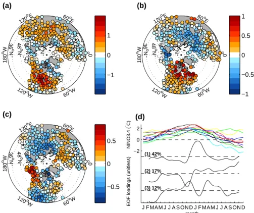
Fig. 1. Singular value decomposition of surface air temperature variability during El Ni˜no events for regions North of 30◦N. (a–c) The spatial patterns (empirical orthogonal functions) associated with modes one through three. Shading indicates the temperature change in degrees Celsius from a one-standard-deviation increase in the corresponding principal component. Note that the two leading patterns indicate a warming concentrated in the interior of northern North America. (d) (top) The NINO3.4 temperature index during a two-year interval for the ten largest El Ni˜no events since 1880. (below) The temporal variability (principal components) associated with modes one through three. Dashed lines indicate the zero-level and percentages indicate the relative amount of variance each mode describes. Note that the second principal component has a positive loading during the second half of the El Ni˜no interval, suggesting that an El Ni˜no event causes northern North America to warm during the ablation season.
of a coupled GCM to changes in tropical temperatures and concluded that warming the eastern equatorial Pacific would have a small influence on North American glaciation on the basis of small changes in the global annual mean tempera-ture. More locally, however, warming the eastern equatorial Pacific in their model appears to warm the high-latitudes of North America by as much as 5◦C in the winter and 2◦C
in the summer (Haywood et al., 2007, Fig. 1b) – consistent with other studies (Barreiro et al., 2006). Investigation of the local North American temperature response, as well as the structure of the full seasonal cycle, seems necessary prior to drawing conclusions regarding El Ni˜no’s influence on glacia-tion.
As simple as a warmer eastern tropical Pacific may seem for accounting for the absence of icesheets before ∼3 Ma, it needs to be reconciled with a fundamental component of Milankovitch’s hypothesis – that summer ablation must in-crease. El Ni˜no teleconnections are clearly documented to cause winter warming in North America (e.g. Ropelewski and Halpert, 1986; Trenberth et al., 1998), but to increase
ablation of ice, summer – not winter – must warm. This co-nundrum motivates us to explore the influence of El Ni˜no on the full seasonal cycle of temperature in North America and then to extrapolate this relationship to past climates.
While our focus is on eastern tropical Pacific tempera-tures, other components of the climate could also contribute to, or themselves explain, the absence of glaciation in North America during the early Pliocene. Such components in-clude higher concentrations of greenhouse gases (e.g. Hay-wood et al., 2005), greater ocean transport of heat (e.g. Rind and Chandler, 1991), or decreased precipitation in response to a less stratified North Pacific (Haug et al., 2005) . But the strong evidence that the eastern tropical Pacific was warmer during the early Pleistocene prompts our consideration of whether this warming and the associated climatic teleconnec-tions could alone account for the absence of North American glaciation. The calculation is in the spirit of what might be done on the back of envelope – with the aim of estimating whether eastern equatorial Pacific cooling could lower sum-mer ablation sufficiently to permit initiation of glaciation.
We begin by making an empirical estimate of the high-latitude temperature response to El Ni˜no events using em-pirical data. The analysis relies mostly upon the Global His-torical Climatology Network (GHCN) (Peterson and Vose, 1997), which provides daily resolution instrumental temper-ature. As the GHCN records give only daily maximum and minimum temperature, we use the average of these two to estimate daily average temperature. The GHCN network has recently been updated through 2006, and most records ex-tend back to at least 1950 and some as far back as 1850. Note, in particular, that El Ni˜no events are associated with small variations in precipitation and snow accumulation at high-latitudes, so that discussion is focused on temperature. The extra-tropical temperature response is analyzed in three steps:
Identification: The strength of El Ni˜no is estimated by av-eraging the sea-surface-temperature anomalies (Kaplan et al., 1998) over the NINO3.4 region, between 120◦W and 170◦W and within 5◦of the equator, yielding a NINO3.4 index. Af-ter smoothing the NINO3.4 index with a five-month running mean, we selected the ten largest temperature excursions. These largest temperature excursions demarcate “El Ni˜no in-tervals”, defined to begin in January of 1877, 1888, 1902, 1905, 1940, 1972, 1982, 1986, 1991, and 1997 and to extend for two years, thus encapsulating the period of anomalous eastern equatorial Pacific SSTs. (If instead of ten events, five or fifteen are selected, the results do not change.)
Extra-tropical response: We average as many of the ten El Ni˜no intervals as are present in each GHCN temperature record into a single, composite El Ni˜no interval. Averaging helps to suppress random temperature variability and thus isolate the consistent extra-tropical response to an El Ni˜no event. (Later, we return to these averages, as well the stan-dard deviation between El Ni˜no intervals, when discussing ablation.) Only records from the northern extra-tropics that span at least one El Ni˜no event are included, giving 363 records with, on average, 62 years of daily observations.
Time/space description: A singular value decomposi-tion (e.g. von Storch and Zwiers, 1999) of the 363 com-posite El Ni˜no intervals yields the spatial and temporal pat-terns which “explain” the greatest possible variance of extra-tropical temperatures. Our primary interest is in the low-frequency temperature response to warming in the eastern equatorial Pacific. Thus, we first smooth each composite temperature record using a 90 day tapered running average to suppress synoptic scale variations while still retaining the seasonal temperature variability. We also truncate the first and last 45 days of the record (i.e. half the length of the smoothing window) so that the retained points are equally smoothed. The first three principal component / empirical or-thogonal function pairs (PC/EOF) are readily interpreted (see Fig. 1). The leading PC/EOF pair, accounting for 42% of the temperature variance, indicates warming between December
1900 1920 1940 1960 1980 2000 −1.5 −1 −0.5 0 0.5 1 1.5 year temperature anomaly ( °C) −1 0 1 −1 0 1 2 NINO3.4 index (°C)
high−latitude temp. anom. (
°C
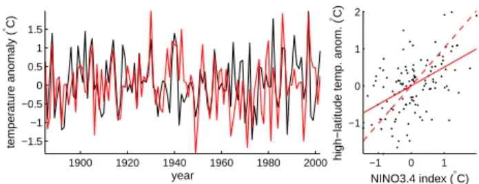
Fig. 2. (Left) Tropical Pacific (black) and high-latitude continental (red) temperature anomalies. Tropical temperature anomalies from the NINO3.4 region are averaged between June to May and high-latitude temperature anomalies from continental stations between 160◦W and 55◦W and North of 50◦N are averaged between De-cember to November. Both time-series are plotted against the year associated with December. (Right) The cross-correlation between the NINO3.4 index and high-latitude temperature anomalies is 0.5. A least-squares fit of the linear trend (solid line) yields a slope of 0.5, and a bias-corrected estimate of the slope yields 1 (dashed line).
and March, and is concentrated in the interior of North Amer-ica at mid-latitudes. Note that at mid-latitudes winter tem-perature can breach the freezing point and can be associated with modest changes in ablation.
The second PC/EOF pair, which explains 17% of the tem-perature variance, indicates warmer temtem-peratures through-out northern North America during the second year of the El Ni˜no interval. This sustained high-latitude warm-ing of North America appears the most pertinent with re-gard to glaciation. We checked this relationship further by comparing the NINO3.4 index with northern North Amer-ican surface air temperatures from the Climate Research Unit’s monthly resolved temperature compilation (Jones and Moberg, 2003). (To be specific, we define the region between 130◦W and 70◦W and north of 50◦N as the high-latitudes or northern North America.) These data reach back to 1885, earlier than most GHCN records. For the NINO3.4 index we took the annual average for the period from June to May (the warmest El Ni˜no months), and for the surface air tempera-tures we used the average between January and December (consistent with the warm phase of the second PC).
After detrending both time-series, the cross-correlation between the surface air temperature and NINO3.4 between 1885 and 2005 is 0.5 (Fig. 2). Monte Carlo experiments, ac-counting for the autocorrelation in both time-series, indicate this correlation is significant at the 99% confidence level. A least-squares estimate of the slope treating the NINO3.4 in-dex as the independent variable and high-latitude tempera-tures as the dependent variable yields 0.5, but this is biased low owing to noise in the NINO3.4 index. A simple correc-tion is to divide the slope by the cross-correlacorrec-tion (see Sokal and Rohlf, 1981; Frost and Thompson, 2000), giving a bias corrected slope of 1, but this assumes that the two quanti-ties covary perfectly, and is biased high. The slope estimates of 1 and 1/2 are thus indicative of upper and lower bounds.
552 P. Huybers and P. Molnar: Tropical temperature and glaciation 120 o W 60 oW 0 o 60o E 120 oE 180 o W 50 o N 60 o N 70 o N 80 o N (a) −20 −10 0 10 20 120 o W 60 oW 0 o 60o E 120 oE 180 oW 50 o N 60 o N 70 o N 80 o N (b) 1000 2000 3000 4000 120 o W 60oW 0 o 60o E 120 oE 180 o W 50 o N 60 o N 70 o N 80 o N (c) −1 0 1 120 o W 60oW 0 o 60o E 120 oE 180 oW 50 o N 60 o N 70 o N 80 o N (d) −200 0 200
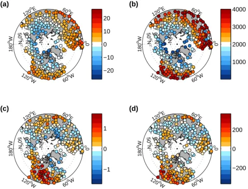
Fig. 3. (a) Mean annual temperature in◦C for regions North of 40◦N from the GHCN database (Peterson and Vose, 1997), (b) the number of positive-degree-days in◦C-days, and (c, d) their respective anomalies during El Ni˜no events. Temperature and PDD anomalies are the December to November average of the ten largest El Ni˜nos intervals since 1880, or fewer, if the record begins after 1880.
(Reassuringly, the conclusions we later come to hold within a factor-of-two range in the sensitivity of northern North America to tropical temperatures.)
The third PC/EOF, which accounts for 12% of the vari-ance, is the final useful descriptor of temperature variability – subsequent PC/EOF pairs explain less than 6% of the vari-ance. The third PC/EOF most closely resembles the time-evolution of the NINO3.4 temperature during an El Ni˜no event – excepting the January to February negative excur-sion. Measures of teleconnections with El Ni˜no that rely upon a linear fit with NINO3.4 tend to emphasize this mode, giving the incorrect impression that El Ni˜no warming in North America is confined to the margins (see e.g. Halpert and Ropelewski, 1992). In actuality, PC/EOF pairs one and two show not only that warming is greatest in the interior of North America, but also that some warming occurs dur-ing the sprdur-ing, summer, and fall – suggestdur-ing that the eastern tropical Pacific could influence glaciation. A similar analysis performed using only North American temperature records yields these same conclusions.
3 Temperature and ablation
Surface temperature reconstructions in the eastern Equatorial Pacific indicate a long-term cooling trend of approximately four degrees Celsius since four million years ago (e.g. Rav-elo et al., 2004; Wara et al., 2005; Lawrence et al., 2006).
The simplest approach to estimating the extra-tropical re-sponse is to assume that in the past the eastern equatorial Pacific was uniformly warmer throughout the year, and that the annual average warming observed for NINO3.4 is propor-tional to a constant temperature change in the extra-tropical Northern Hemisphere. We estimate the proportionality as the ratio of the annual average (December to November) land temperature anomaly to the annual average (June to May) NINO3.4 temperature during the ten largest El Ni˜no events. The NINO3.4 (Fig. 1) and northern North American temper-ature anomalies (Fig. 3c) both average ∼1◦C, giving a ratio
of ∼1, as might be expected from EOFs one and two (Fig. 1) and from the bias-corrected regression between the NINO3.4 index and average temperature in northern North America (Fig. 2).
Is it reasonable to extrapolate El Ni˜no’s influence on high-latitude temperature to the case of a constantly warmer east-ern Equatorial Pacific? Two recent general circulation model simulations permit comparison: (1.) Barreiro et al. (2006) impose an approximately four degree Celsius annual average warming on the eastern Equatorial Pacific as well as warm-ing in the Indian and Atlantic oceans and obtain approxi-mately four degrees of annual average warming in the in-terior of northern North America, thus simulating a tempera-ture response in close agreement with our extrapolation both in terms of spatial distribution and magnitude (see our Fig. 3c and their Fig. 8) and (2.) Haywood et al. (2007) impose an
Pacific on a background climate that is already made warmer than the present, and they obtain a northern North Ameri-can warming of about two degrees in the winter and half a degree in the summer, thus yielding an annual average mag-nitude roughly half that of our extrapolation, but referenced to a different background climate state. We conclude that our temperature extrapolation is consistent with model sim-ulations to within a factor of two.
High-latitude temperature anomalies, of themselves, do not indicate changes in ablation simply because warmer tem-peratures that are still sub-freezing do not much affect tion. To quantify the influence of daily temperature on abla-tion we use positive degree days (PDDs),
PDD =XδdTd. (1)
Td is the daily temperature and δd is zero if Td<0◦C and
one otherwise. The composite El Ni˜no intervals, however, come from averages over different years, and the distribution of temperature around this average needs to be accounted for (see Braithwaite, 1984). For example, if the average temper-ature on January first hovers just below freezing, the expected PDDs are nonetheless positive because some realizations of January first temperature will inevitably exceed freezing. We assume a normal distribution with a standard deviation cal-culated from, for example, all January first temperatures in a record. The expected number of PDDs becomes,
< PDD >= 365 X d=1 Z ∞ 0 xγ ( ¯Td, σd, x)dx. (2)
γ is a normal distribution of temperature with mean ¯T and standard deviation σ on day d, and x is temperature in Cel-sius integrated from the freezing point upward. All PDDs reported in this paper are the expected values, but with the brackets left off for simplicity. For stations where seasonal temperatures hover near freezing, PDDs calculated using Eq. (2) exceed those using Eq. (1) by as much as 50%.
PDDs tend to be smallest at high-latitudes and in the in-terior of continents. A one degree annual average rise in the NINO3.4 index – corresponding to a moderate El Ni˜no event – is associated with, on average, a 90◦C-day increase in northern North America (Fig. 3d). Note that peak differ-ences in PDDs lie south of peak differdiffer-ences in temperature because more days breach the freezing point to the south. PDDs increase super-linearly with temperature because both the magnitude increases and the number of days with positive temperatures increases. Thus, assuming that extra-tropical temperatures continue to scale linearly with the NINO3.4 index, a 2◦C warming in the NINO3.4 region is associated with a 300◦C-day increase; a 4◦C tropical warming gives a 630◦C-day increase, but this pushes the limits of plausibility in extrapolating teleconnections from large modern El Ni˜no events to climates that include a warmer eastern equatorial
slightly in the interior and increase slightly near the margins. Common scaling factors relating ablation rates (in terms of water equivalent thickness) to PDDs range from 3 mm/(day◦C) for snow-covered surfaces to 8 mm/(day◦C) for bare ice (Braithwaite and Zhang, 2000; LeFrebre et al., 2002). The higher rate of ice ablation owes to a lower albedo. Thus a 300 (day◦C) increase in northern North America cor-responds to an ablation rate higher by one to two meters per year than today. Considering that for the modern cli-mate northern North America receives an average of 0.4 m of precipitation per year (according to GHCN records, Peter-son and Vose, 1997), such a large increase in ablation would presumably inhibit glaciation.
So far we have assumed that the response to eastern trop-ical Pacific warming is constant through the seasons, as a simplest possible case, but a seasonally varying response is perhaps more realistic. Furthermore, paleoceanographic ob-servations of past temperatures are usually spaced at cen-turies or longer, and therefore cannot resolve ENSO ity over shorter durations, let alone 3-7 years, if such variabil-ity is present at all. Thus we cannot distinguish whether the long-term decline in eastern equatorial temperatures owes to a shift in mean temperature or to decreases in the frequency or amplitude of El Ni˜no events (e.g. Haywood et al., 2007). To explore the implications of seasonal temperature variabil-ity – as opposed to a constant response across the seasons – we perturbed each extra-tropical temperature record by a sea-sonally varying temperature anomaly. Specifically, we add to the temperature on each day of a record the temperature anomaly on the corresponding day in the composite El Ni˜no interval, taken between December to November. The result-ing increase in PDDs is actually somewhat larger for northern North America than that obtained from the annual average scaling described earlier. Thus, the inference of greater abla-tion in response to a warmer eastern equatorial Pacific holds assuming either the seasonally varying temperature pertur-bation associated with modern El Ni˜no events or a constant annual warming.
In contrast to our line of reasoning, Kukla et al. (2002) suggest that El Ni˜no conditions will increase the moisture supply to North America and, thus, actually promote glacia-tion. Using the same procedure of averaging temperature for the ten largest El Ni˜no intervals but now for precipitation, we find that precipitation increases in North America by no more than 10 cm/year between 25◦to 50◦N, and that at higher
lat-itudes precipitation increases by less than 1cm/year. These observational results appear consistent with the simulation of Barreiro et al. (2006, their Fig. 7). While changes in pre-cipitation almost certainly contribute to changes in the mass balance of North American icesheets, we estimate El Ni˜no increases the magnitude of ablation by more than a factor of ten relative to changes in precipitation. Thus, as is generally the case for glaciers and icesheets (e.g. Paterson, 1994), we anticipate ablation to exert the primary control on glaciation.
554 P. Huybers and P. Molnar: Tropical temperature and glaciation 120 o W 60 oW 0 o 60o E 120 oE 180 oW 50 o N 60 o N 70 o N 80 o N (a) 0.9 0.92 0.94 0.96 0.98 1 120 o W 60 oW 0 o 60o E 120 oE 180 oW 50 o N 60 o N 70 o N 80 o N (b) 0.02 0.04 0.06 0.08 0.1 0.12 120 o W 60oW 0 o 60o E 120 oE 180 oW 50 o N 60 o N 70 o N 80 o N (c) 20 30 40 50 120 o W 60oW 0 o 60o E 120 oE 180 oW 50 o N 60 o N 70 o N 80 o N (d) 0 100 200 300
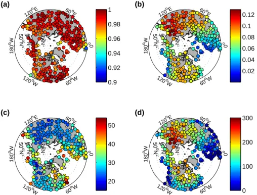
Fig. 4. The temperature and positive degree day (PDD) response to changes in insolation at latitude North of 40◦N. (a) The squared-cross-correlation between lagged insolation and the average seasonal cycle in temperature. (b) The sensitivity of temperature to insolation, in units of◦C/(W/m2). (c) The number of days temperature lags incoming insolation at the top of the atmosphere. (d) The calculated difference in PDDs resulting from changing the tilt of Earth’s spin axis, or its obliquity, from 22.2◦to 24.2◦, an amount similar to the amplitude of an average obliquity cycle.
4 Comparison with insolation
The magnitude of the tropically-induced changes in PDDs can be placed in context by comparison with the effects of Earth’s orbital variations. If changes in Earth’s orbital con-figuration, and the resulting shifts in insolation, force North America between unglaciated and glaciated states, then the difference in ablation between orbital configurations associ-ated with glacial and interglacial periods indicates the forc-ing required to preclude glaciation. Two factors complicate simple application of this logic. First, glacial cycles might occur independent of orbital variation and are perhaps only paced by changes in insolation (e.g. Tziperman et al., 2006). Such self-sustained oscillation seem most relevant for the ∼100 kyr late Pleistocene glacial cycles, but the early Pleis-tocene 40 kyr glacial cycles appear to respond directly to ra-diative forcing, with the timing and amplitude of changes in glaciation closely following the insolation integrated over the summertime (Huybers, 2006). As the integrated summer en-ergy is almost wholly a function of obliquity, we use the dif-ference in PDDs between low and high obliquity to gauge the forcing required to preclude glaciation.
The second complication is that feedbacks – for exam-ple, involving ice-albedo, icesheet instabilities, greenhouse gases, or ocean and atmospheric circulation shifts – could
amplify the glacial response to insolation variability. Fur-thermore, Liu and Herbert (2004) found that eastern tropical Pacific temperatures covary with obliquity and the extent of glaciation, confounding separation of orbital and tropical Pa-cific influences on glaciation. Insofar as climate feedbacks contribute only after ice is growing, however, their effects are irrelevant with respect to the onset of glaciation.
Earth’s orbital variations are well-known over the last 5Ma (e.g. Berger and Loutre, 1992), and these have been specified within a general circulation model (Jackson and Broccoli, 2003) and, more simply, energy balance models (e.g. Huy-bers and Tziperman, 2007) to determine the sensitivity of PDDs. Our experiments with energy balance models, how-ever, indicate that the relationship between solar insolation and temperature can be winnowed down to three parameters – a lag, L; sensitivity, S; and constant, B – and we opt for a very simple representation,
Ti(d + L) = SiI (d, φi) + Bi, (3)
In words, the lagged daily average temperature, T (d+L), at station i is related to daily average insolation, I (d, φ), by a sensitivity, S, and a constant temperature, B. φi is the
lati-tude at which temperature is recorded. The average cross-correlation obtained between Eq. (3) and the average sea-sonal cycle at each site is 0.99 (Fig. 4a) – as high as could be
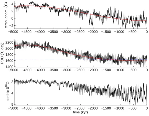
−5000 −4500 −4000 −3500 −3000 −2500 −2000 −1500 −1000 −500 0 −2 0 2 4 temp. anom. ( ° C −5000 −4500 −4000 −3500 −3000 −2500 −2000 −1500 −1000 −500 0 1400 1600 1800 2000 2200 PDD ( ° C day) −5000 −4500 −4000 −3500 −3000 −2500 −2000 −1500 −1000 −500 0 3 4 5 time (kyr) benthic δ 18 O
Fig. 5. Glacial implications of tropical cooling. (top) Alkenone derived SST anomalies for the eastern equatorial Pacific (from Lawrence et al., 2006), normalized so that the most recent estimate is 0◦C. Red line indicates the long-term trend, fit using a third-order polynomial. (middle) Calculated average positive degree days for northern North America (between 70◦W and 130◦W and above 50◦N) obtained by applying temperature perturbations expected to result from tropical anomalies (red line) and also including orbital variations (black line). For reference, the lowest number of PDDs obtained by 2.7 Ma is indicated (dashed line). (bottom) A combination of many benthic δ18O records (Lisiecki and Raymo, 2005), where more positive values indicate greater ice-volume. Note the y-axis is reversed.
obtained through fitting an energy-balance-model. Eastern continental interiors show the greatest sensitivity and least lag with insolation, presumably because these regions are the most isolated from the buffering effects of the oceans.
We expect the relationship between temperature and in-solation estimated using modern observations to hold under different orbital configurations, at least to first order, because the variations in insolation are small relative to the mean and are concentrated at the seasonal cycle. For example, shift-ing obliquity from 22.2◦ to 24.2◦ causes an increase in the amplitude (measured from maximum to minimum intensity) of the annual cycle at 65◦N of 40 W/m2but only a 6 W/m2 change in the annual mean insolation. In the case of pre-cession, shifting perihelion from winter to summer solstice causes an increase in the amplitude of the annual cycle by 54 W/m2and the annual mean insolation is invariant.
Assuming that the relationship between temperature and insolation (Eq. 3) estimated from modern data holds under different configurations of Earth’s orbit, we calculate the temperature at these sites for the seasonal cycles when obliq-uity is 22.2◦ and 24.2◦. PDDs are calculated from temper-ature using Eq. (2). The specified two-degree increase in obliquity is a typical amplitude for an obliquity cycle and, according to our calculations, causes an average increase of 170◦C-days in northern North America. Jackson and
Broc-coli (2003) obtain a similar result from their GCM calcu-lation. The amount by which PDDs change in response to changes in obliquity depends on the local change in insola-tion and the sensitivity of temperature to changes in inso-lation. Thus the PDD response to an increase in obliquity is largest in continental interiors, away from the buffering effects of the ocean, and at high latitudes where obliquity-induced difference in insolation are greatest.
Finally, we consider the combined influence of tropical temperature and orbital variations. As our interest is in dis-cerning if the long-term eastern tropical Pacific temperature changes could have initiated glaciation, we fit a third order polynomial to the 5Myr temperature record of Lawrence et al. (2006). This fit indicates an overall cooling of 4◦C, and
we use this as a proxy for the decrease in the NINO3.4 index. The anomalies in the NINO3.4 proxy are used to calculate extra-tropical temperature changes, as described in Sect. 3. The orbitally-forced temperature changes over the last 5 Ma are calculated as described in Sect. 4, in this case includ-ing changes in obliquity, precession, and eccentricity (Berger and Loutre, 1992). Figure 5 shows the variations in PDDs from the combined tropical- and insolation-forced tempera-ture response, assuming that the modern standard deviations in temperature also hold for the past.
556 P. Huybers and P. Molnar: Tropical temperature and glaciation
∼600◦C-days, much larger than the ∼170◦C-days
associ-ated with variations in obliquity (Fig. 5). The steepest trop-ically induced change in PDDs occurs between 3.5 Ma and 2.5 Ma, coinciding with a rapid increase in the δ18O of ben-thic foraminifera, and which Mudelsee and Raymo (2005) associated with the onset of Northern Hemisphere glacia-tion. Although the modern estimate of the ratio between tropical and high-latitude warming need not hold under much warmer tropical conditions, the tropical forcing appears suffi-ciently strong that even were its influence decreased by a fac-tor of two, it would still be larger than the obliquity-induced changes in PDDs.
5 Conclusions
According to Milankovitch’s hypothesis, summer ablation must dip below a threshold value for glaciation to initiate. Our calculations indicate that the decline in eastern tropical Pacific temperatures since ∼5Ma would decrease ablation in northern North America by more than twice as much as orbitally-induced changes, and thus could readily bring the climate close enough to glaciation such that, during a favor-able orbital configuration, an icesheet would form. We thus conclude that tropical cooling appears sufficient to switch North America from an unglaciated state to one with inter-mittent glaciations. Understanding the puzzle of what caused the eastern equatorial Pacific to cool off on a timescale too long to invoke the atmosphere-ocean-cryosphere system by itself now appears all the more pressing.
Acknowledgements. We thank J. C. H. Chiang and G. Roe for
helpful discussion as well as M. Cane, F. Peeters, C. Wunsch, and an anonymous reviewer for useful comments on earlier drafts of this manuscript.
Edited by: F. Peeters
References
Barreiro, M., Philander, G., Pacanowski, R., and Fedorov, A.: Sim-ulations of warm tropical conditions with application to middle Pliocene atmospheres, Clim. Dyn., 26, 349–365, 2006.
Berger, A. and Loutre, M. F.: Astronomical solutions for paleocli-mate studies over the last 3 million years, Earth Planet. Sci. Lett., 111, 369–382, 1992.
Braithwaite, R.: Calculation of degree-days for glacier-climate re-search, Zeitschrift fur Gletscherkunde und Glazialgeologie, 20, 1–8, 1984.
Braithwaite, R. and Zhang, Y.: Sensitivity of mass balance of five Swiss glaciers to temperature changes assessed by tuning a degree-day model, J. Glaciology, 152, 7–14, 2000.
Cane, M.: A role for the tropical Pacific, Science, 282, 59–60, 1998. Cane, M. and Molnar, P.: Closing of the Indonesian seaway as a precursor to east African aridification around 3−4 million years ago, Nature, 411, 157–162, 2001.
Fedorov, A., Dekens, P., McCarthy, M., Ravelo, A., deMenocal, P., Barreiro, M., Pacanowski, R., and Philander, S.: The Pliocene Paradox (Mechanisms for a Permanent El Ni˜no), Science, 312, 1485–1489, 2006.
Frost, C. and Thompson, S.: Correcting for regression dilution bias: comparison of methods for a single predictor variable, Journal of the Royal Statistical Society, 163, 173–190, 2000.
Halpert, M. and Ropelewski, C.: Surface temperature patterns as-sociated with the Southern Oscillation, J. Climate, 5, 577–593, 1992.
Haug, G., Ganopolski, A., Sigman, D., Rosell-Mele, A., Swann, G., Tiedemann, R., Jaccard, S., Bollmann, J., Maslin, M., Leng, M., and Eglinton, G.: North Pacific seasonality and the glaciation of North America 2.7 million years ago, Nature, 433, 821–825, 2005.
Haywood, A., Dekens, P., Ravelo, A., and Williams, M.: Warmer tropics during the mid-Pliocene? Evidence from alkenone paleothermometry and a fully coupled ocean-atmosphere GCM, Geochem. Geophys. Geosyst., 6, Q03010, doi:10.1029/2004GC000799, 2005.
Haywood, A., Valdes, P., and Peck, V.: A permanent El Ni˜no-like state during the Pliocene?, Paleoceanography, 22, PA1213, doi:10.1029/2006PA001323, 2007.
Huybers, P.: Early Pleistocene glacial cycles and the integrated summer insolation forcing, Science, 313, 508–511, 2006. Huybers, P. and Tziperman, E.: Integrated summer insolation
forc-ing and 40 000 year glacial cycles: the perspective from an icesheet/energy-balance model, Paleoceanography, in press. Imbrie, J., Boyle, E. A., Clemens, S. C., Duffy, A., Howard, W. R.,
Kukla, G., Kutzbach, J., Martinson, D. G., McIntyre, A., Mix, A. C., Molfino, B., Morley, J. J., Peterson, L. C., Pisias, N. G., Prell, W. L., Raymo, M. E., Shackleton, N. J., and Toggweiler, J. R.: On the structure and origin of major glaciation cycles. 1. Linear Responses to Milankovitch Forcing, Paleoceanography, 7, 701–738, 1992.
Jackson, C. and Broccoli, A.: Orbital forcing of Arctic cli-mate: mechanisms of climate response and implications for continental glaciation, Clim. Dyn., 21, 539–557, doi:10.1007/ s00382-003-0351-3, 2003.
Jones, P. and Moberg, A.: Hemispheric and large-scale surface air temperature variations: An extensive revision and an update to 2001, J. Climate, 16, 206–223, 2003.
Kaplan, A., Cane, M., Kushnir, Y., Clement, Y., Blumenthal, M., and Rajagopalan, B.: Analyses of global sea surface temperature 1856-1991, J. Geophys. Res., 103, 18 567–18 589, 1998. Kukla, G., Clement, A., Cane, M. Gavin, J., and Zebiak, S.: Last
interglacial and early glacial ENSO, Quat. Res., 58, 27–31, doi: 10.1029/2002PA000837, 2002.
Lawrence, K., Liu, Z., and Herbert, T.: Evolution of the Eastern Tropical Pacific Through Plio-Pleistocene Glaciation, Science, 312, 79–83, 2006.
Lefebre, F., Gallee, H., Van Ypersele, J., and Huybrechts, P.: Modeling of large-scale melt parameters with a regional climate model in South-Greenland during the 1991 melt season, Ann. Glaciol., 35, 391–397, 2002.
Liu, Z. and Herbert, T.: High latitude signature in Eastern Equato-rial Pacific Climate during the Early Pleistocene Epoch, Nature, 427, 720–723, 2004.
Lisiecki, L. and Raymo, M.: A Pliocene-Pleistocene stack of 57
PA1003, doi:10.1020/2004PA001071, 2005.
Milankovitch, M.: Kanon der Erdbestrahlung und seine Andwen-dung auf das Eiszeitenproblem, Royal Serbian Academy, Bel-grade, 1941.
Molnar, P. and Cane, M.: El Ni˜no’s tropical climate and teleconnec-tions as a blueprint for pre-Ice Age climates, Paleoceanography, 17(2), 1021, doi:10.1029/2001PA000663, 2002.
Mudelsee, M. and Raymo, M.: Slow dynamics of the North-ern Hemisphere glaciation, Paleoceanography, 20, PA4022, doi:10.1029/2005PA001153, 2005.
Paterson. W. Physics of Glaciers. Pergamon Press, 3rd edition, 1994.
Peterson, T. and Vose, R.: An overview of the Global Historical Climatology Network temperature database, Bull. Am. Meteorol. Soc., 78, 2837–2849, 1997.
Philander, G. and Fedorov, A.: Role of tropics in changing the re-sponse to Milankovitch forcing some three million years ago, Pa-leoceanography, 1045, doi:10.1029/2002PA000837, 2003. Ravelo, A., Andreasen, D., Lyle, M., Lyle, A., and Wara, M.:
Re-gional climate shifts caused by gradual global cooling in the Pliocene epoch, Nature, 429, 263–267, 2004.
Ravelo, A., Dekens, P., and McCarthy, M.: Evidence for El Ni˜no-like conditions during the Pliocene, GSA Today, 16(3), 4–11, 2006.
the Pliocene?, Science, 307, 1948–1952, 2005.
Rind, D. and Chandler, M.: Increased ocean heat transports and warmer climate, J. Geophys. Res., 96, 7437–7461, 1991. Ropelewski, C. and Halpert, M.: North American precipitation and
temperature patterns associated with the El Ni˜no/Southern Oscil-lation, Monthly Weather Review, 114, 2352–2362, 1986. Storch, v. H. and Zwiers, F.: Statistical analysis in climate research,
Cambridge University Press, 1999.
Sokal, R. and Rohlf, F. Biometry, 2nd edition, Freeman, 1981. Trenberth, K., Branstator, G., Karoly, D., Kumar, A., Lau, N., and
Ropelewski, C.: Progress during TOGA in understanding and modeling global teleconnections associated with tropical sea sur-face temperatures, J. Geophys. Res., 103, 14 291–14 324, 1998. Tziperman, E., Raymo, M., Huybers, P., and Wunsch, C.:
Conse-quences of pacing the Pleistocene 100 kyr ice ages by nonlinear phase locking to Milankovitch forcing, Paleoceanography, 21, PA4206, doi:doi:10.1029/2005PA001241, 2006.
Wara, M., Ravelo, C., and Delaney, M.: Permanent El Ni˜no-like conditions during the Pliocene warm period, Science, 309, 758– 761, 2005.
Zachos, J., Pagani, M., Sloan, L., Thomas, E., and Billups, K.: Trends, Rhythms, and Aberrations in Global Climate 65 Ma to Present, Science, 292, 686–693, 2001.