Supplemental Materials for
Scaling of the Fano effect of the in-plane Fe-As phonon and the superconducting
critical temperature in Ba
1−xK
xFe
2As
2B. Xu,1,∗ E. Cappelluti,2 L. Benfatto,3 B. P. P. Mallett,1, 4 P. Marsik,1 E. Sheveleva,1 F. Lyzwa,1
Th. Wolf,5 R. Yang,6 X. G. Qiu,6 Y. M. Dai,7 H. H. Wen,7 R. P. S. M. Lobo,8, 9 and C. Bernhard1,†
1
University of Fribourg, Department of Physics and Fribourg Center for Nanomaterials, Chemin du Mus´ee 3, CH-1700 Fribourg, Switzerland
2
Istituto di Struttura della Materia, CNR, 34149 Trieste, Italy 3
ISC-CNR and Department of Physics, Sapienza University of Rome, P.le A. Moro 5, 00185 Rome, Italy 4The Photon Factory, Department of Physics, University of Auckland, 38 Princes St, Auckland, New Zealand 5
Institute of Solid State Physics, Karlsruhe Institute of Technology, Postfach 3640, Karlsruhe 76021, Germany 6
Beijing National Laboratory for Condensed Matter Physics, Institute of Physics, Chinese Academy of Sciences, Beijing 100190, China 7
National Laboratory of Solid State Microstructures and Department of Physics, Nanjing University, Nanjing 210093, China 8
LPEM, ESPCI Paris, PSL University, CNRS, F-75005 Paris, France 9Sorbonne Universit´e, CNRS, LPEM, F-75005 Paris, France
OPTICAL RESPONSE IN BKFA AND TEMPERATURE DEPENDENCE OF THE PHONON AND ITS PARAMETERS OBTAINED FROM THE FANO FIT
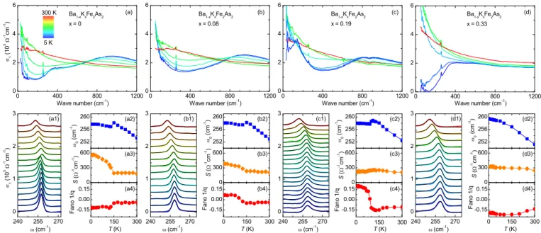
The upper panels of Figure S1 show the temperature dependent spectra of the real part of the optical conductivity,
σ1(ω), in the infrared range for selected doping levels of x = 0, 0.08, 0.19 and 0.33. Their infrared conductivity is
dominated by the strong electronic response that is composed of a Drude peak at the origin, due to the itinerant carriers, and a pronounced tail toward high frequency, that arises from inelastic scattering of the free carriers and/or low-lying interband transitions [1–4]. The spectra agree well with the previously reported ones [5–10] and show the well-known changes due to the spin-density-wave (SDW) at TN = 138 K, 130 K and 90 K for x = 0, 0.08 and 0.19, respectively, and the SC gap below Tc = 18 K, and 38 K at x = 0.19 and 0.33, respectively. The SDW and the SC gaps both reduce the spectral weight of the regular charge carrier response. For the former this spectral weight is shifted to higher energy, where it forms a so-called pair-breaking peak, whereas in the SC state it is transferred to a
δ(ω) function at the origin that accounts for the infinite dc conductivity.
The temperature dependence of the phonon parameters ω0, S and 1/q, obtained from the Fano fits, is shown in
the lower right panels of Fig. S1. For all magnetic samples, the combined AF and structural transition into the o-AF state gives rise to clear anomalies in the T -dependence of ω0, S and, especially, of 1/q. At x = 0, in agreement with
previous reports [11, 12], 1/q has a very small negative value in the paramagnetic state that increases strongly in magnitude below TN (Fig. S1(a4)). For the doped samples with x = 0.08 and 0.19 the o-AF transition gives rise to corresponding anomalies, except that 1/q increase from a negative value above TN (that is larger at x = 0.19 than at 0.08) to a large positive value below TN. Finally, for the optimally doped sample without any AF order (x = 0.33, Fig. S1(d4)) 1/q has the largest negative value and it is only weakly temperature dependent. Quite remarkably, there is hardly a signature of the SC transition at Tc in the temperature dependence of the phonon parameters. This is a clear indication that the Fano effect of the Eu Fe-As mode does not arise from the coupling with the itinerant charge carriers, for which the spectral weight in the vicinity of the phonon mode decreases below Tc due to the formation of the SC energy gap. This implies that the Fano effect of this Eu phonon mode is governed by the coupling to some interband transitions that are part of the electronic background at higher frequency (that is only weakly affected by the SC transition as shown in Fig. S1(d)).
0 400 800 1200 0 2 4 240 255 270 0 1 2 3 252 256 260 0 300 600 0 150 300 -0.15 0.00 0.15 0 400 800 1200 0 2 4 0 400 800 1200 0 2 4 0 400 800 1200 0 2 4 240 255 270 0 1 2 3 252 256 260 0 300 600 0 150 300 -0.15 0.00 0.15 252 256 260 0 300 600 0 150 300 -0.15 0.00 0.15 252 256 260 0 300 600 0 150 300 -0.15 0.00 0.15 240 255 270 0 1 2 3 240 255 270 0 1 2 3 5 K 300 K x = 0 Ba 1-x K x Fe 2 As 2 1 ( 1 0 3 -1 c m -1 ) W ave number (cm -1 ) 0.000 150.0 300.0 (a1) 1 ( 1 0 3 -1 c m -1 ) (cm -1 ) (a2) 0 ( c m -1 ) (a3) S ( -1 c m -1 ) (a4) F a n o 1 / q T (K) Ba 1-x K x Fe 2 As 2 x = 0.08 W ave number (cm -1 ) Ba 1-x K x Fe 2 As 2 x = 0.19 W ave number (cm -1 ) Ba 1-x K x Fe 2 As 2 x = 0.33 W ave number (cm -1 ) (b1) (cm -1 ) 0 ( c m -1 ) (b2) (b3) (b4) S ( -1 c m -1 ) T (K) F a n o 1 / q 0 ( c m -1 ) (c2) (c3) (c4) S ( -1 c m -1 ) T (K) F a n o 1 / q 0 ( c m -1 ) (d2) (d3) (d4) S ( -1 c m -1 ) T (K) F a n o 1 / q (d1) (cm -1 ) (c1) (cm -1 )
FIG. S1: (color online) Temperature dependent optical conductivity of Ba1−xKxFe2As2 in the far infrared region for x = 0
(a), 0.08 (b), 0.19 (c) and 0.33 (d). (a1–d1) Line shape of the infrared-active phonon mode (with offset) at temperatures from 300 to 5 K (color lines). The underlying black solid lines through the data denote the corresponding Fano fit. Temperature dependence of the (a2–d2) phonon frequency ω0, (a3–d3) strength S and (a3–d3) Fano parameter 1/q of the phonon for x = 0, 0.08, 0.19 and 0.33 in Ba1−xKxFe2As2.
FITTING OF THE ELECTRONIC BACKGROUND AND ITS EFFECT ON THE FANO PARAMETER
The reflectivity data of BKFA were acquired with the same resolution of 4 cm−1 on the Bruker Vertex 70v. To check the effect of the resolution on the phonon lineshape, we have measured the spectra for the x = 0.33 sample with different resolutions at 150 K. The differences of the phonon lineshape are detailed in Figure S2(a) and Figure S2(b). Clearly, the phonon linewidth is strongly dependent on the resolution, whereas the Fano parameter 1/q2 remains almost unchanged. For a comparison, in Figure S2(b) we also included a symmetric phonon lineshape with 1/q2= 0. Compared to the symmetric phonon lineshape, the change of the phonon lineshape due to the asymmetry effect spans a wide frequency range that is several times larger than the phonon linewidth. Therefore, the resolution used in our measurement is sufficient to capture the asymmetry of the phonon mode and thus its Fano parameter.
Figure S2(c) shows, for the case of the x = 0.33 sample at 150 K, how different low-frequency extrapolations during the Kronig-Kramers analysis of R(ω) influence the obtained spectra of σ1(ω). It shows that it mostly affects the
low-frequency region below the phonon mode. Figure S2(d) highlights the corresponding changes in the region around the phonon mode and shows that the lineshape of the phonon mode is only weakly affected. The thin solid lines through the data are fits of the Fano line shape which confirm that the value of the Fano parameter, 1/q2, does not strongly
depend on the low-frequency extrapolation. This observation agrees with our finding that the Fano effect of the FeAs mode does not arise from a coupling to the itinerant charge carriers but rather involves some interband transitions that are located on the high-energy side of the phonon.
Generally, σ1(ω) of pnictides can be modeled over a wide frequency range with a superposition of several Drude
and Lorentz components. The black line in Fig. S2(e) shows such a wide range Drude-Lorentz fit of the electronic background for which the additional phonon mode has been fitted by a Fano line shape. However, in order to accurately capture the characteristics of the phonon with such a wide range fit, it would be required that the spectra are essentially noiseless. A more reliable and accurate approach that has been used in this manuscript is therefore based on fitting the spectra in a narrow frequency range centered around the phonon mode for which the electronic background can be reasonably well described with a linear or quadratic function. Figure. S2(f) shows the corresponding Fano fits of the phonon mode with the linear (blue line) or quadratic (green) background at x = 0.33 and T = 150 K. Figure S2(g) shows the corresponding temperature dependence of the Fano parameter 1/q2 obtained from the fits
with the linear and quadratic backgrounds. Finally, Fig. S2(h) displays the corresponding doping dependence of the Fano parameter 1/q2 at 150 K as obtained from the fits with the linear (red symbols) and quadratic (black symbols)
0 200 400 600 0 2 4 6 8 240 255 270 3.0 3.3 3.6 240 255 270 3.0 3.3 3.6 0 100 200 300 0.00 0.02 0.04 0.06 0 10 20 30 40 50 60 0.00 0.02 0.04 0.06 0 200 400 600 800 0 2 4 6 240 255 270 3.0 3.2 3.4 3.6 3.8 4.0 240 255 270 0.0 0.2 0.4 0.6 (c) Constant Hagen-Rubens Marginal-Fermi-Liquid Two-f luid 1 ( 1 0 3 -1 cm -1 ) x = 0.33 T = 150 K (d) Wave number (cm - 1 ) C onstant (1/q 2 = 0.039) H agen-R ubens (1/q 2 = 0.042) M arginal-Fermi-Liquid (1/q 2 = 0.043) Two-f luid (1/q 2 = 0.044) 1 ( 1 0 3 -1 cm -1 ) (f) Wave number (cm - 1 ) x = 0.33 1 ( 1 0 3 -1 cm -1 ) 150 K Linear (1/q 2 = 0.046) Quadratic(1/q 2 = 0.042) (g) x = 0.33 Linear Quadratic 1 / q 2 Temperature (K) (h) Quadratic Linear 1 / q 2 K% in Ba 1- x K x Fe 2 As 2 T = 150 K (e) x = 0.33 1 ( 1 0 3 -1 cm -1 ) 150 K Drude-Lorentz (1/q 2 = 0.052) x = 0.33 T = 150 K 1 cm -1 2 cm -1 4 cm -1 1 ( 1 0 3 -1 cm -1 ) Resolution (a) (b) 1 cm - 1 1/q 2 = 0.049 2 cm - 1 1/q 2 = 0.049 4 cm - 1 1/q 2 = 0.048 1/q 2 = 0 1 ( 1 0 3 -1 cm -1 ) Wave number (cm - 1 )
FIG. S2: (color online) (a) Phonon lineshape measured with different resolutions. (b) Phonon lineshape after the background is subtracted. The solid line through the data is the Fano fit. (c)The optical conductivity at x = 0.33 obtained by the Kronig-Kramers analysis of R(ω) with different low-frequency extrapolations, such as Constant (R(ω) = constant), Hagen-Rubens (R(ω) = 1− A√ω), Marginal Fermi Liquid (R(ω) = 1− Aω), and Two Fluid (R(ω) = 1 − Aω2). Panel (d) shows the enlarged view of panel (c) focusing on the phonon around 255 cm−1. The solid lines show the Fano fits obtained with a quadratic description of the electronic background. Panel (e) shows for the spectrum obtained with a Hagen-Rubens extrapolation how the Fano fit and the Fano parameter of the phonon mode are affected if the electronic background is fitted over a wide frequency range with a Drude-Lorentz model. Panel (f) shows the Fano fits of the phonon when the electronic background is fitted over a narrow range around the phonon mode, either with a linear (blue) or quadratic (green) function. Panel (g) shows the temperature dependence of the Fano parameter 1/q2 obtained from the fits with the linear and quadratic backgrounds at
x = 0.33. Panel (h) displays the corresponding doping dependence of the Fano parameter 1/q2at 150 K obtained from the fits with the linear and quadratic backgrounds. It confirms that its characteristic dome-like doping dependence does not depend on the details of the fitting procedure
In particular, it highlights that characteristic doping dependence of 1/q2 in the paramagnetic state (at T ≥ 150 K) is an intrinsic feature that does not depend on the fitting of the electronic background. The variation of 1/q2 for the different backgrounds is in fact included in the error bar of 1/q2, as shown in Fig. 2(d) of the main text.
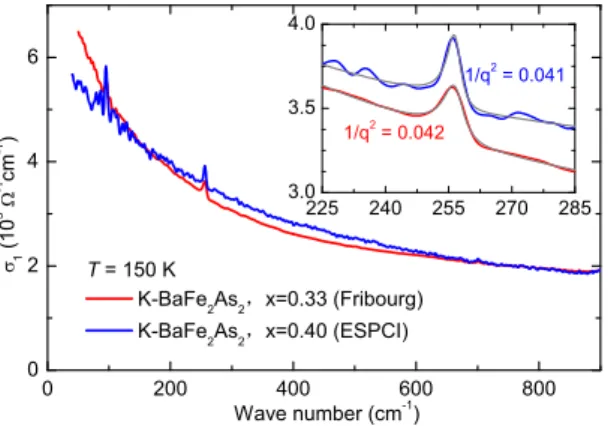
0 200 400 600 800 0 2 4 6 225 240 255 270 285 3.0 3.5 4.0 1 ( 1 0 3 -1 cm -1 ) K-BaFe 2 As 2 x=0.33 (Fribourg) K-BaFe 2 As 2 x=0.40 (ESPCI) 1/q 2 = 0.041 W ave number (cm -1 ) T = 150 K 1/q 2 = 0.042
FIG. S3: (color online) Optical conductivity, at 150 K, of Ba0.67K0.33Fe2As2(presented in the main text) and Ba0.6K0.4Fe2As2 (measured at ESPCI). The inset shows the phonon and its Fano fit at 150 K for both samples. It confirms that the value of the obtained Fano-parameter does not strongly depend on the noise level of the spectra.
In Fig. S3 we compare the Fano fitting for the σ1(ω) spectra at 150 K of the optimally doped Ba0.67K0.33Fe2As2
sample from the manuscript and the more noisy spectrum of a Ba0.6K0.4Fe2As2 crystal with a similarly high Tc that
(b)
M
X
Y
Γ
Γ
M
(a)
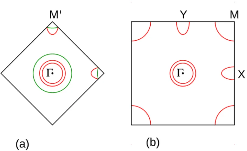
FIG. S4: (color online) (a) Sketch of typical Fermi surfaces at low doping in iron-based pnictides in the reduced Brillouin zone corresponding to two Fe and two As atoms per unit cell. Red and green Fermi surfaces have different symmetries and no optical transition is allowed among them. (b) Sketch of Fermi surfaces like in panel (a) in the extended Brillouin zone corresponding to one Fe and one As atom per unit cell. Green Fermi sheets in panel (a) are obtained upon folding of panel (b) in the reduced Brillouin zone.
the obtained Fano parameter hardly depend on the experimental setup the noise level of the spectra. The inset shows that in both cases the asymmetric phonon line shape can be seen directly in the bare spectra and the fitting hardly depends on the noise level.
HAMILTONIAN AND OPTICAL ELECTRONIC TRANSITIONS IN UNFOLDED BRILLOUIN ZONE
As a suitable tool for investigating the electronic and optical excitations of iron-based cuprates in the presence of a Eu lattice distortion, we consider for the moment the 5-band tight-binding model based on the Slater-Koster approach, as discussed for instance in Ref. [14]. Relevant orbitals are thus the 5 d Fe-orbitals and the 3 p As orbitals. In this scheme, considering the layer Fe-As, inter-atomic electronic hoppings between Fe atoms contaning direct Fe-Fe hopping terms and As-mediated hoppings which can be evaluated within the second order perturbation theory.
Considering the staggered vertical positions of the A atoms, the formal unit cell contains two Fe atoms, and hence the Hilbert space should contains 5+5 d-orbitals for a total of 10 bands. Such unit cell is conventionally used in first-principle calculations and the resulting bands are depicted in the corresponding square Brillouin zone, whose corners are M′= (±π, 0)/a, (±π, 0)/a, a being the Fe-Fe distance (see Fig. S4). Typical Fermi surfaces, in this framework, for the undoped case, contain two electron-like Fermi pockets at the M′points, with zx/xy (yz/xy) orbital character, and two hole-like Fermi sheets around the Γ point with mainly zx/yz. A further hole-band at Γ with main xy character can driven at the Fermi level depending on doping and on the out-of-plane height of the As atom.
Although this picture is commonly reported in first-principle based calculations, the band structure can be more conveniently viewed in the unfolded Brillouin zone, which correspond to consider one Fe atom per cell. The possibility of such unfolding was discussed analytically in a detailed way in Ref. [14]. The crucial point is that the 10× 10 Hamiltonian can be divided, choicing an appropriate Hilbert space, in two 5× 5 separate blocks with different symmetry: ˆ H10×10(k) = ( ˆ H5×5(k) ˆ0 ˆ H Hˆ5×5(k + Q) ) , (1)
where Q = (π, π)/a. As discussed in Ref. [14], each 5× 5 block can be obtained as a result of a simplest tight-binding model defined in a unit cell containing only one Fe atom, and hence with a corresponding larger square Brillouin zone defined by the corners M=(±π, ±π)/a. Since the two blocks are orthogonal, and since the second block can be obtained just as a shift k→ k + Q. The band-structure of (1) can be simply obtained from the band-structure of the block ˆH5×5(k) upon a “folding”, as shown in Fig. S4. Due to the orthogonality of the two blocks, the
elliptical electronic Fermi pockets result to be degenerate (in the absence of spin-orbit interaction) along the M-M line. The effective possibility of low-energy excitations between these two degenerate bands is however not trivial since
it involves coupling between electronic states with opposite symmetry. In particular, it is straightforward to realize that the current operator, for instance along x, ˆjx(k), which can be obtained as derivative ˆjx(k) = ∂ ˆH(k)/∂kx, does not couple to states belonging to different 5× 5 blocks. Low-energy excitations associated to the band-crossing of the electronic bands are thus not allowed in the optical conductivity and, in general, no particle-hole optically active continuum can be obtained at energies as low as the Eu phonon energy ω≈ 250 cm−1 in a Fermi surface scenario as the one depicted in Fig. S4 representative of undoped/low-doped BKFA. As a consequence, since the charged-phonon response function χ(ω) contains a subselection of the optically active transitions of the electronic background [15–17], no sizable Fano effect can be observed (apart the small one induced by the residual intraband scattering), in agreement with our observation at x = 0 in the normal state T > TN.
Entering a appropriate broken symmetry phase (tuning the temperature below TN), or changing the Fermi surface topology provide two different and independent ways to induces a sizable Fano effect.
Concerning the effects of a broken symmetry phase, it should be stressed that the forbidding of low-energy opti-cal active transitions between band-crossing electronic bands strongly relies on the possibility of splitting the total Hamiltonian in two separate orthogonal 5×5 blocks. Such splitting is itself possible as a consequence of the symmetry of the lattice, electronic and magnetic degrees of freedom in the normal state. Under these conditions, the initial two Fe atoms per cell can be mapped in two indepedent lattices of only one Fe atoms per cell. It is clear that any breaking of these conditions will induce the need of an effective two Fe-atoms per cell, i.e . will induce an effective coupling between the two 5× 5 blocks, and hence te low-energy optical transitions between the electronic bands that are responsible for a sizable Fano effect. This is clearly the case of the stripe-like antiferromagnetic order o-AF for
T < TN where the magnetic/lattice ordering make the two Fe atoms inequivalent. Different broken symmetry phases can have of course different effects on the newly allowed low-energy optical transition, and this is reflected in the anomaly observed in the Fano effect about x≈ 0.24 − 0.26 where a different magnetic order t-AF enter into play.
Note that not every broken symmetry phase can be responsible for the activation of new optical channels, but only phases that break the underlying symmetries that make possible the “unfolding” process, and the reduction from two Fe atoms per cell to one Fe atom per cell. On this regards it is clear that the superconducting ordering act in a different (Nambu) space and it does not change the relevant symmetries of the normal states. On this ground, entering the superconducting phase is not expected to affect the relevant optical transitions for ω > 2∆, and hence not to affect the Fano properties, in accordance with our observations.
Electron or hole doping, changing the topology of the Fermi sheets, can provide also a suitable way of inducing and tuning a finite sizable Fano effect. It has been recently suggested that in hole-doped BKFA, due to the relative different upwards and downwards shifts of the hole-like and electron-like bands, the Fermi surface scenario can be quite different from the one typical of undoped compound, and the optimal doping can occur when the elliptical electron-like Fermi surfaces evolve in electron-like propeller shapes, as described in Refs. [18, 19]. Additional hole doping can leads also to hole-like propellers, passing through a region where unavoidably the Fermi level crosses a Dirac point. In such scenario, like in graphene, low-energy optical transitions, within each of the 5× 5 block, are known to be finite and relevant, and are the natural candidate for a finite sizable Fano effect in the normal state. Further doping can eventually move the Fermi level far from the Dirac physics and leads to the observed depletion of 1/q2 for x > 0.33.
ELECTRON-PHONON COUPLING AND CHARGED-PHONON RESPONSE OF THE Eu MODE IN
LAYERED IRON-BASED PNICTIDES
In order to shed further light on the microscopic mechanism responsible for the Fano effect of the Eu in the normal state, and to reveal a crucial dependence on the orbital content, we present here a microscopic analysis of the charged-phonon response function using a tight-binding model that permits to identify the crucial orbital character.
Basic ingredient for the microscopical analysis of the changed-phonon response function are: i) the
multi-band/multi-orbital electronic Hamiltonian ˆH(k); ii) the current operator that can be derived in a straightforwward
way (for instance along the x-axis) as ˆJx(k) = d ˆH(k)/dk
x; iii) and the electron-phonon matrix term ˆV (k) coupling the electronic states with the q = 0 Eu lattice distortion.
We have already discussed above how in the normal state both Hamiltonian and the current operator can be divided in two 5× 5 independent blocks. Few more words are worth to be spent about such electron-phonon coupling. After a careful analysis, it is clear to see that the in-plane Eu lattice distortion, depicted in Fig. S5, does not break the relevant symmetries and the normal state and it does not hence mix the two 5× 5 blocks. This supports the analysis that low-energy optical transitions at the Euphonon energy ω ∼ 250 cm−1must be sought in the intra-block allowed optical transitions. It should be stressess however that this scenario has not a general validity of a generic phonon
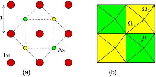
(b)
As
Fe
(a)
u
a
Ω
2Ω
1FIG. S5: (color online) (a) Lattice structure of the Fe-As plane. Fe atoms (big red circles) form a square lattice (with lattice constant a) whereas As atoms (small colored circles) lie at the center in a staggered out-of-plane position, respectively depicted as yellow and green. The dotted squared represents the natural unit cell of containing two Fe atoms and two As atoms, while the dashed square depicts the reduced unit cell containing just one Fe atom and one As atoms. Such reduced unit cell is suitable in a convenient basis where Bloch states with different symmetries are decoupled, as discussed in the main text. (b) Sketch of the lattice structure upon Eufrozen phonon distortion u. Yellow and green squares represent Fe plaquettes with staggered As
out-of-plane position. Ω1, Ω2 denote the set of Slater-Koster parameters for the two inequivalent bonds in the presence of a
Eudistortion.
mode. Most evident is the case of the out-of-plane A2u optical mode that involves a rigid upward (or downward)
shift of all the As atoms with respect to the Fe plane. The two As atoms result thus to have different z heights from Fe plane and to be thus deeply not equivalent. As a consequence the electron-phonon coupling associated with such optical mode cannot be divided in two separated 5× 5 blocks and it will induce low-energy transitions between the two electron-like elliptical Fermi sheets in the undoped case.
On the ground of these results, focusing on the Eu phonon mode, we can restrict our further analysis on one single 5× 5 block and investigate how it is affected by a rigid in-plane shift of the As atoms. The Slater-Koster approach is particular suitable to this aim since lattice distortions can be modelled in terms of few simple parameters describing the change of the direction cosines and the amplitude change of the hopping energies. For sake of simplicity we retain in our analysis only the relevant orbital components in the hole-doped range here considered, namely the zx, yz and
xy orbitals. zx and yz are expected to be dominant for the hole-like bands close to the Γ point, whereas a mix of zx + xy (yz + xy) orbitals will be relevant for the electron-pockets close to the X (Y) points, respectively.
From a general point of view, we can write: ˆ
H(k; u) = ˆHFe(k) + ˆHAs(k; u), (2)
where ˆHFe(k) represents the direct hopping between Fe atoms, and ˆHAs(k; u) the second order As-mediated processes,
which will be affected by the Eu distortion quantified by the lattice displacement u. Denoting as “A” and “B” the two inequivalent Fe sublattices, we introduce the Hilbert space defined the vector
Φi(k) = (dA,zx(k), dA,yz(k), dA,xy(k), dB,zx(k), dB,yz(k), dB,xy(k), ) . (3) In this Hilbert space each term ˆHi(k; u) (i = Fe, As) can be written as a 6× 6 Hamiltonian, namely:
ˆ Hi(k; u) = ( ˆ Hi,AA(k; u) Hˆi,AB(k; u) ˆ Hi,BA(k; u) ˆHi,BB(k; u) ) , , (4)
where the 3× 3 Hamiltonian ˆHAA(k) represents the next-nearest neighbor hopping Hamitonian only among Fe sublattice A, ˆHBB(k) the 3×3 next-nearest neighbor hopping Hamiltonian connecting only Fe atoms on the sublattice B, and ˆHAB(k), ˆHBA(k) the nearest-neighbor hopping between the two sublattices. Note that ˆHAB(k), ˆHBA(k) connect only atoms along the x/y axis whereas ˆHAA(k), ˆHBB(k) only atoms along the diagonal of the Fe square lattice.
Considering first direct Fe-Fe hopping, we can write thus: ˆ HFe(k) = ( ˆ Hd Fe(k) Hˆ x/y Fe (k) ˆ HFex/y(k) Hˆd Fe(k) ) , (5) where ˆ HFed (k) = γ d zx,zx4cxcy −γzx,yzd 4sxsy 0 −γd yz,zx4sxsy γyz,yzd 4cxcy 0 0 0 γdxy,xy4cxcy, , (6) ˆ HFex/y(k) = γ x zx,zx2cx+ γzx,zxy 2cy 0 0 0 γx yz,yz2cx+ γyz,yzy 2cy 0
0 0 γx/yxy,xy2(cx+ cy),
, (7)
and where cx= cos(kxa), cy = cos(kxy), sx= sin(kxa), sy = sin(kxy), γzx,zxd = γyz,yzd = [Uddπ(
√
2a) + Uddδ(√2a)]/2,
γd xy,xy = [3Uddσ( √ 2a) + Uddδ( √ 2a)]/4, γd zx,yz = γdyz,zx = [Uddπ( √ 2a)− Uddδ( √ 2a)]/2, γx zx,zx = γyz,yzy = γ x/y xy,xy =
Uddπ(a), and γzx,zxy = γyz,yzx = Uddδ(a). Here Uddσ(R), Uddπ(R), Uddδ(R) represent the Slater-Koster Fe-Fe energy integrals at the distances R = a for nearest neighbors, and R =√2a for next-nearest neighbors.
Our main focus in this paper is the modulation of the As-mediated effective hopping between Fe atoms upon a Eu lattice distortion. We will focus for the moment on the As-mediated hopping processes connecting one Fe atom on the sublattice A with neighbor Fe atoms on the sublattices A and B, i.e. on the blocks ˆHAA(k; u) and ˆHAB(k; u). The remaining blocks ˆHBB(k; u), ˆHBA(k; u) will be evaluated later using symmetry arguments. We denote with
Ω = {r, θ, ϕ} the set of the relevant parameters in the context of Slater-Koster model, namely d being the
inter-atomic distance between Fe and As atom, and θ and ϕ1 the direction cosines pointing from the Fe to the As atom.
In the presence of a Eu lattice distortion, we need to employ two different sets Ω1, Ω2, as depicted in Fig. S5. For
sake of simplicity, following Ref. [14], we denote ϵd the local energy of the Fe d-orbitals, and ϵp the local energy of the As p-orbitals, neglecting the energy splitting due to the crystal field. Fe d orbitals are denoted with the label
α, β = zx, yz, xy whereas As p orbitals are denoted with the label µ = x, y, z.
It is also useful to introduce the function
tα,β(Ω1, Ω2) = ∑ µ=x,y,z tα,µ(Ω1)tµ,β(Ω2) ϵd− ϵp . (8)
With this notation, the As-mediated hopping between the α and β d-orbitals of nearest-neighbor Fe atoms along the x, y axes, with α being on the A sublattice, will be:
txα,β(k; Ω1, Ω2) = [tα,β(d1, θ1, α1; d2,−θ2,−α2) + tα,β(d1,−θ1,−α1; d2, θ2, α2)] eikxa
+ [tα,β(d2, π + θ2, α2; d1, π− θ1,−α1) + tα,β(d2, π− θ2,−α2; d1, π + θ1, α1)] e−ikxa, (9)
tyα,β(k; Ω1, Ω2) = [tα,β(d1, θ1, α1; d1, π− θ1,−α1) + tα,β(d2, π− θ2,−α2; d2, θ2, α2)] eikya
+ [tα,β(d1,−θ1,−α1; d1, π + θ1, α1) + tα,β(d2, π + θ2, α2; d2,−θ2,−α2)] e−ikya, (10)
whereas the hopping terms between next-neighbor Fe atoms along the diagonal of the square Fe-lattice will obey the relations:
tdα,β(k; Ω1, Ω2) = tα,β(d1θ1, α1; d2, θ2,−α2)eikxa+ikya+ tα,β(d2, π + θ2, α2; d1, π + θ1,−α1)e−ikxa−ikya
+tα,β(d1,−θ1,−α1; d2,−θ2, α2)eikxa−ikya+ tα,β(d2, π− θ2,−α2; d1, π− θ1, α1)e−ikxa+ikya.(11)
After few straightforward steps, using the symmetry properties of the Slater-Koster energy integrals, we can write the general expression for the As-mediated hopping Hamiltonian in the presence of the Eulattice distortion. Focusing on the 3× 3 “AA” block describing the hopping processes along the diagonal of the Fe square lattice, we can write:
ˆ
HAs,AA(k; u) =
t
d
zx,zx4cxcy tdR,zx,yz2sxsy+ itdI,zx,yz2cxsy tdR,zx,xy2cxcy+ itdI,zx,xy2sxcy
td
R,yz,zx2sxsy+ itdI,yz,zx2cxsy tdyz,yz4cxcy tdR,yz,xy2sxsy+ itdI,yz,xy2cxsy
tdR,xy,zx2cxcy+ itdI,xy,zx2sxcy tdR,xy,yz2sxsy+ itdI,xy,yz2cxsy tdxy,xy4cxcy
,(12)
× 3 “AB” block describing the hopping processes along the x/y axis the Fe square lattice we have: ˆ HAs,AB(k; u) = t x
zx,zx2cx+ tyzx,zx2cy 0 txR,zx,xy2cx+ itxI,zx,xy2sx+ tyzx,xy2cy
0 tx
yz,yz2cx+ tyyz,yz2cy ityyz,xy2sy
tx
R,xy,zx2cx+ itxI,xy,zx2sx+ tyxy,zx2cy ityxy,yz2sy txxy,xy2cx+ tyxy,xy2cy,
. (13)
Slater-Koster parameters Ω1, Ω2. Their explicit expressions read: txzx,zx(Ω1, Ω2) = − ∑ µ=x,y,z gµx2tµ,xz(Ω1)tµ,xz(Ω2) ϵd− ϵp , , (14) tyzx,zx(Ω1, Ω2) = ∑ µ=x,y,z gyµ[tµ,xz(Ω1)tµ,xz(Ω1) + tµ,xz(Ω2)tµ,xz(Ω2)] ϵd− ϵp , (15) txyz,yz(Ω1, Ω2) = ∑ µ=x,y,z gxµ2tµ,yz(Ω1)tµ,yz(Ω2) ϵd− ϵp , (16) tyyz,yz(Ω1, Ω2) = − ∑ µ=x,y,z
gµy[tµ,yz(Ω1)tµ,yz(Ω1) + tµ,yz(Ω2)tµ,yz(Ω2)] ϵd− ϵp , (17) tdzx,zx(Ω1, Ω2) = ∑ µ=x,y,z gzµtµ,zx(Ω1)tµ,zx(Ω2) ϵd− ϵp , (18) tdyz,yz(Ω1, Ω2) = ∑ µ=x,y,z gzµtµ,yz(Ω1)tµ,yz(Ω2) ϵd− ϵp , (19) tdR,zx,yz(Ω1, Ω2) = tdR,yz,zx(Ω1, Ω2) = ∑ µ=x,y,z gxµgyµ[tµ,zx(Ω1)tµ,yz(Ω2) + tµ,zx(Ω2)tµ,yz(Ω1)] ϵd− ϵp , (20) tdI,zx,yz(Ω1, Ω2) = −tdI,yz,zx(Ω1, Ω2) =− ∑ µ=x,y,z gµxgµy[tµ,zx(Ω1)tµ,yz(Ω2)− tµ,zx(Ω2)tµ,yz(Ω1)] ϵd− ϵp , (21) txxy,xy(Ω1, Ω2) = − ∑ µ=x,y,z gµx2tµ,xy(Ω1)tµ,xy(Ω2) ϵd− ϵp , (22) tyxy,xy(Ω1, Ω2) = ∑ µ=x,y,z
gxµgµz[tµ,xy(Ω1)tµ,xy(Ω1) + tµ,xy(Ω2)tµ,xy(Ω2)] ϵd− ϵp , (23) tdxy,xy(Ω1, Ω2) = ∑ µ=x,y,z gxµgµytµ,xy(Ω1)tµ,xy(Ω2) ϵd− ϵp , (24) txR,zx,xy(Ω1, Ω2) = −txR,xy,zx(Ω1, Ω2) = ∑ µ=x,y,z gµygµz[tµ,zx(Ω1)tµ,xy(Ω2)− tµ,zx(Ω2)tµ,xy(Ω1)] ϵd− ϵp , (25) txI,zx,xy(Ω1, Ω2) = txI,xy,zx(Ω1, Ω2) = ∑ µ=x,y,z gµygµz[tµ,zx(Ω1)tµ,xy(Ω2) + tµ,zx(Ω2)tµ,xy(Ω1)] ϵd− ϵp , (26) tyzx,xy(Ω1, Ω2) = −tyxy,zx(Ω1, Ω2) = ∑ µ=x,y,z gxµgzµ[tµ,xz(Ω1)tµ,xy(Ω1)− tµ,xz(Ω2)tµ,xy(Ω2)] ϵd− ϵp , (27) tdR,zx,xy(Ω1, Ω2) = tdR,xy,zx(Ω1, Ω2) = ∑ µ=x,y,z gµxgyµ[tµ,zx(Ω1)tµ,xy(Ω2)− tµ,zx(Ω2)tµ,xy(Ω1)] ϵd− ϵp , (28) tdI,zx,xy(Ω1, Ω2) = −tdI,xy,zx(Ω1, Ω2) = ∑ µ=x,y,z gxµgyµ[tµ,zx(Ω1)tµ,xy(Ω2) + tµ,zx(Ω2)tµ,xy(Ω1)] ϵd− ϵp , (29) tyyz,xy(Ω1, Ω2) = tyxy,yz(Ω1, Ω2) = ∑ µ=x,y,z
gxµgµz[tµ,yz(Ω1)tµ,xy(Ω1) + tµ,yz(Ω2)tµ,xy(Ω2)] ϵd− ϵp , (30) tdR,yz,xy(Ω1, Ω2) = tdR,xy,yz(Ω1, Ω2) = ∑ µ=x,y,z gµz
[tµ,yz(Ω1)tµ,xy(Ω2)− tµ,yz(Ω2)tµ,xy(Ω1)]
ϵd− ϵp , (31) tdI,yz,xy(Ω1, Ω2) = −tdI,xy,yx(Ω1, Ω2) =− ∑ µ=x,y,z gµz
[tµ,yz(Ω1)tµ,xy(Ω2) + tµ,yz(Ω2)tµ,xy(Ω1)]
ϵd− ϵp
, (32)
where gν
µ =−1 if µ = ν and gµν = 1 otherwise.
1→ −α1 2→ −α2 ˆ HAs,BB(k; u) = t d
zx,zx4cxcy tdR,zx,yz2sxsy+ itdI,zx,yz2cxsy −tdR,zx,xy2cxcy− itdI,zx,xy2sxcy
tdR,yz,zx2sxsy+ itdI,yz,zx2cxsy tdyz,yz4cxcy −tdR,yz,xy2sxsy− itdI,yz,xy2cxsy
−td
R,xy,zx2cxcy− itdI,xy,zx2sxcy −tdR,xy,yz2sxsy− itdI,xy,yz2cxsy tdxy,xy4cxcy
, (33) and ˆ HAs,BA(k; u) = t x zx,zx2cx+ t y zx,zx2cy 0 −t x R,zx,xy2cx− it x I,zx,xy2sx− t y zx,xy2cy 0 tx
yz,yz2cx+ tyyz,yz2cy −ityyz,xy2sy
−tx
R,xy,zx2cx− it
x
I,xy,zx2sx− t
y
xy,zx2cy −it y xy,yz2sy t x xy,xy2cx+ t y xy,xy2cy . (34)
Eqs. (5)-(7), along with (12), (13), (33), (34), define the band structure within the Slater-Koster context in the presence of a finite generic Eulattice distortion u. For u = 0 we have{|Ω1|} = {|Ω2|} = {|Ω0|}, where {|Ωi|} = {|Ωj|} means ri = rj, |θi| = |θj| and |ϕi| = |ϕj|. In this limit we recover thus the tight-binding model of Ref. [14] in the reduced zx, yz, xy space. Note that in the perfect crystal structure it was shown (see Ref. [14]) that an appropriate basis to re-write the total Hamiltonian in two separate blocks with different symmetries is defined by the Hilbert space:
Φi(k) = (d+,zx(k), d+,yz(k), d−,xy(k), d−,zx(k), d−,yz(k), d+,xy(k), ) , (35)
where d±α= [dA,zx(k)± dB,zx(k)]/
√
2. One can easily see that, since the Eudistortion does not affect the underlying symmetries on the base of such decoupling in separate blocks, the same Hilbert space (35) can decoupled the total 6× 6 Hamiltonian in two separate 3 × 3 blocks. In such space we have thus:
ˆ H(k; u) = ( ˆ H3×3(k; u) 0 0 Hˆ3×3(k + Q; u) ) , (36) where ˆ H3×3(k; u) = HˆFe(k) + ˆHAs(k; u). (37)
In similar way as above, each matrix ˆHi(k; u) can be divided in hopping terms along the x/y axis and hopping terms along the diagonal. We have thus:
ˆ HFe(k) = Hˆ x/y Fe (k) + ˆH d Fe(k), (38) where ˆ Hx/y Fe (k) = γ x zx,zx2cx− γzx,zxy 2cy 0 0 0 γx
yz,yz2cx− γyz,yzy 2cy 0
0 0 −γxy,xy2(cx/y x+ cy) , (39) ˆ Hd Fe(k) = γ d zx,zx4cxcy −γzx,yzd 4sxsy 0 −γd yz,zx4sxsy γyz,yzd 4cxcy 0 0 0 γd xy,xy4cxcy , (40) and ˆ HAs(k; u) = Hˆ x/y As (k; u) + ˆH d As(k; u), (41) where ˆ Hx/y As (k; u) = t x zx,zx2cx+ t y zx,zx2cy 0 −t x R,zx,xy2cx− it x I,zx,xy2sx− t y zx,xy2cy 0 tx
yz,yz2cx+ tyyz,yz2cy −ityyz,xy2sy
txR,xy,zx2cx+ itxI,xy,zx2sx+ tyxy,zx2cy ityxy,yz2sy −txxy,xy2cx− tyxy,xy2cy
, (42) and ˆ Hd As(k; u) = t d
zx,zx4cxcy tdR,zx,yz2sxsy+ itdI,zx,yz2cxsy tdR,zx,xy2cxcy+ itdI,zx,xy2sxcy
td
R,yz,zx2sxsy+ itdI,yz,zx2cxsy tdyz,yz4cxcy tdR,yz,xy2sxsy+ itdI,yz,xy2cxsy
tdR,xy,zx2cxcy+ itdI,xy,zx2sxcy tdR,xy,yz2sxsy+ itdI,xy,yz2cxsy tdxy,xy4cxcy
.(43)
The decoupling in Eq. (36) of the total Hamiltonian, in the presence of a Eu lattice distortion, in two separate
blocks with different symmetries signalize that the Eu in-plane optical phonon is just coupled to vertical (q = 0) particle-hole transitions in the extended Brillouin zone, and not to the (symmetry forbidden) transitions that couple states at different k points in the extended Brillouin zone and that appear vertical in the reduced Brillouin zone just upon folding. This would be different for instance for the out-of-plane optical A2u mode that effectively breaks the
underlying symmetries and it would induce off-diagonal elements in Eq. (36).
As said, Eqs. (36)-(43) hold true in any generic Eu lattice distortion u. They provide also the basis for obtaining an explicit expression for the linear electron-phonon coupling with the Eu phonon, upon expansion of ˆHAs(k; u) at
the linear order in u, i.e.
ˆ Vep(k) = lim u→0 ˆ HAs(k; u) u . (44)
To this aim we can write
tµ,α(Ω1) ≈ tµ,α(Ω0) + uwµ,α(Ω0), (45)
where wµ,α(Ω0) contains all the contributions coming from the modulation of the energy integrals and from the
modulation of the direction cosines. From symmetry arguments we get also
tµ,α(Ω2) ≈ tµ,α(Ω0)− uwµ,α(Ω0). (46)
One can now realize that most of the hopping terms in Eqs. (14)-(32) have a vanishing linear coupling with u. The only hopping terms that give rise to a linear electron-phonon coupling result to be td
I,zx,yz, t
x
R,zx,xy, t
y
zx,xy, tdR,zx,xy,
tdR,yz,xy. We obtain thus the matrix expression for the electron-phonon coupling: ˆ Vep(k) = ( ˆ V3×3(k) 0 0 Vˆ3×3(k + Q) ) , (47) where ˆ V3×3(k) = 0 iI d
zx,yz2cxsy Izx,xyd 2cxcy− Izx,xyx 2cx− Izx,xyy 2cy
−iId
zx,yz2cxsy 0 Iyz,xyd 2sxsy
Id
zx,xy2cxcy− Izx,xyx 2cxIzx,xyy 2cy Iyz,xyd 2sxsy 0
, (48) and where Izx,yzd = −2 ∑ µ=x,y,z gµxg y µ [wµ,zx(Ω0)tµ,yz(Ω0)− tµ,zx(Ω0)wµ,yz(Ω0)] ϵd− ϵp , (49) Izx,xyx = 2 ∑ µ=x,y,z gyµg z µ [wµ,zx(Ω0)tµ,xy(Ω0)− tµ,zx(Ω0)wµ,xy(Ω0)] ϵd− ϵp , (50) Izx,xyy = 2 ∑ µ=x,y,z gxµg z µ [wµ,xz(Ω0)tµ,xy(Ω0) + tµ,xz(Ω0)wµ,xy(Ω0)] ϵd− ϵp , (51) Izx,xyd = 2 ∑ µ=x,y,z gxµgyµ [wµ,zx(Ω0)tµ,xy(Ω0)− tµ,zx(Ω0)wµ,xy(Ω0)] ϵd− ϵp , (52) Iyz,xyd = 2 ∑ µ=x,y,z gzµ
[wµ,yz(Ω0)tµ,xy(Ω0)− tµ,yz(Ω0)wµ,xy(Ω0)]
ϵd− ϵp
. (53)
Eq. (48) is one of the fundamental ingredients to evaluate on a microscopic ground the charged-phonon response function χ(ω) which is repsonsible for the Fano effect. Other ingredient are the total Hamiltonian ˆH(k; u = 0) in the absence of the lattice distortion and the current operator.
The direct Fe-Fe Hamiltonian term hopping ˆHFe(k) is of course not affected by the lattice distortion, where the
As-mediated term ˆHAs(k; u = 0) = ˆH
x/y
As (k; u = 0) + ˆHdAs(k; u = 0) is simplified for u = 0 as:
ˆ Hx/y As (k; u = 0) = t x
zx,zx2cx+ tyzx,zx2cy 0 −itxI,zx,xy2sx
0 txyz,yz2cx+ tyyz,yz2cy −ityyz,xy2sy
itxI,xy,zx2sx ityxy,yz2sy −txxy,xy2cx− tyxy,xy2cy
ˆ Hd As(k; u = 0) = t d zx,zx4cxcy tdR,zx,yz2sxsy itdI,zx,xy2sxcy td
R,yz,zx2sxsy tdyz,yz4cxcy itdI,yz,xy2cxsy
itdI,xy,zx2sxcy itdI,xy,yz2cxsy tdxy,xy4cxcy
, (55)
where the hopping terms are evaluated at{Ω1} = {Ω2} = {Ω0}.
The current operator along the x-axis can be now also evaluated as ˆJx(k) = d ˆH(k)/dkx. We obtain: ˆ Jx (k) = ( ˆ J3×3(k) 0 0 Jˆ3×3(k + Q) ) , (56) where ˆ J3×3(k) = Jˆ x/y Fe (k) + ˆJ d Fe(k) + ˆJ x/y As (k) + ˆJ d As(k) (57) and where ˆ Jx/y Fe (k) = −γ x zx,zx2sx 0 0 0 −γx yz,yz2sx 0 0 0 γxy,xy2sxx/y , (58) ˆ Jd Fe(k) = −γ d zx,zx4sxcy −γzx,yzd 4cxsy 0 −γd yz,zx4cxsy −γyz,yzd 4sxcy 0 0 0 −γd xy,xy4sxcy , (59) ˆ Jx/y As (k) = −t x zx,zx2sx 0 −it x I,zx,xy2cx 0 −tx yz,yz2sx 0 itxI,xy,zx2cx 0 txxy,xy2sx , (60) ˆ Jd As(k) = −t d zx,zx4sxcy tdR,zx,yz2cxsy itdI,zx,xy2cxcy td
R,yz,zx2cxsy −tdyz,yz4sxcy −itdI,yz,xy2sxsy
itd
I,xy,zx2cxcy −itdI,xy,yz2sxsy −tdxy,xy4sxcy
. (61)
We can build up the charged-phonon function χ(ω) that rules the Fano effect. It is at this stage much more convenient to work in the Matsubara frequency space, whereas the analytical continuation on the real axis can be easily performed later. We have thus:
χ(iωm) = C∑
k,n
Tr [
ˆ
J (k) ˆG(k, iωn+ iωm) ˆVep(k) ˆG(k, iωn)
]
, (62)
where C is a constant, ˆG(k, z) = [(z + µ)ˆI − ˆH(k)]−1, and µ is the chemical potential. Note that all the matrix quantities are separated in two independent 3× 3 blocks. Since the second block is equivalent to the first one upon substitution k → k + Q, we can restrict our analysis to the first block allowing k to span over the whole extende Brillouin zone, covering thus all k’s as well all k + Q’s.
To get a deeper insight, let us assume now that the xy orbital is irrelevant. We can thus restrict our analysis to the 2× 2 block defined by the orbitals zx, yz. In this Hilbert space we have (we drop now the label “3 × 3”):
ˆ H(k) = HI(k) ˆI +Hz(k)ˆσz+Hx(k)ˆσx, (63) ˆ J (k) = JI(k) ˆI +Jz(k)ˆσz+Jx(k)ˆσx, (64) ˆ V(k) = iVy(k)ˆσy, (65)
where ˆσx, ˆσy, ˆσz are Pauli matrices, and where HI(k) = HI,dcxcy+HI,x/y(cx+ cy), Hx(k) =Hx,dsxsy, Hz(k) =
microscopical expressions ofHI,d, HI,x/y,Hx,d, Hz,x/y, JI,d, JI,x/y,Jx,d,Jz,x/y,Vy,d in terms of the Slater-Koster parameters can be inferred from Eqs.(39)-(40), (48), (54)-(61). In similar way, also the Green’s function ˆG(k, z) can be expanded in the Pauli matrix basis. We have in particular: ˆG(k, z) = GI(k, z) ˆI +Gz(k, z)ˆσz+Gx(k, z)ˆσx, where GI(k, z) = [z + µ− HI(k)]/D(k, z), Gx(k, z) = −Hx(k)/D(k, z), Gz(k, z) = −Hz(k)/D(k, z), and where
D(k, z) = [z + µ− HI(k)]2− H2x(k)− Hz2(k) = [z + µ− E1(k)][z + µ− E2(k)]. Here E1(k), E2(k) are the two bands
of the two-band model with zx, yz orbitals:
E1(k) = HI(k) + ∆(k), (66)
E2(k) = HI(k)− ∆(k), (67)
where
∆(k) = √H2
x(k) +H2z(k). (68)
A crucial remark here is that Tr[ ˆJ (k)ˆV(k)] = 0. This implies that we cannot pick up the component ˆG(k, z) ∝
GI(k, z) ˆI in both Green’s functions in Eq. (62). Taking into account the symmetry properties encoded in the Pauli matrix commutation rules, we get thus:
χ(iωm) = −2C ∑
k,n
[Jx(k)GI(k, iωn+ iωm)Vy(k)Gz(k, iωn)]
+2C∑
k,n
[Jx(k)Gz(k, iωn+ iωm)Vy(k)GI(k, iωn)]
+2C∑
k,n
[Jz(k)GI(k, iωn+ iωm)Vy(k)Gx(k, iωn)]
−2C∑
k,n
[Jz(k)Gx(k, iωn+ iωm)Vy(k)GI(k, iωn)]
= 2C∑
k,n
1
D(k, iωn)D(k, iωn+ iωm)
[Jx(k)[iωn+ iωm− HI(k)]Vy(k)Hz(k)]
−2C∑
k,n
1
D(k, iωn)D(k, iωn+ iωm)
[Jx(k)Hz(k)Vy(k)[iωn− HI(k)]]
2C∑
k,n
1
D(k, iωn)D(k, iωn+ iωm)[Jz(k)Hx(k)Vy(k)[iωn− HI(k)]]
−2C∑
k,n
1
D(k, iωn)D(k, iωn+ iωm)[Jz(k)[iωn+ iωm− HI(k)]Vy(k)Hx(k)] = 2iωmC
∑
k,n
Vy(k) [Jx(k)Hz(k)− Jz(k)Hx(k)]
D(k, iωn)D(k, iωn+ iωm) = 4iωmC ∑ k,n Vy(k) [Jx(k)Hz(k)− Jz(k)Hx(k)] f (E1(k)− µ) − f(E2(k)− µ) ∆(k) [(iωm)2− ∆2(k)] . (69)
We can now perform the analytical continuation iωm→ ω + iδ. For ω > 0 we get:
χ”(ω) = −2πC∑
k,n
Vy(k) [Jx(k)Hz(k)− Jz(k)Hx(k)]f (E1(k)− µ) − f(E2(k)− µ)
ω δ(ω− ∆(k)). (70)
Given the orbital content of the electronic band-structure, particle-hole excitations between zx and yz orbitals are allowed close to the X, Y points and in the anular area kF,2≤ k ≤ kF,1 close to the Γ point, where kF,1, kF,2 are the
Fermi momenta associated respectively to the larger (band E1(k)) and smaller (band E1(k)) hole Fermi sheets.
It is easy to see that the coherence factorVy(k) [Jx(k)Hz(k)− Jz(k)Hx(k)] changes sign for k→ k + Q, so that the contributions from the X and Y points cancel out.
Focusing on the parabolic-like hole bands centered at the Γ point, and denoting kx= k cos ψ, kx= k sin ψ, we can expand the coherence factorVy(k) [Jx(k)Hz(k)− Jz(k)Hx(k)] at the leading order (∝ k4). We get:
∫ d2kVy(k) [Jx(k)Hz(k)− Jz(k)Hx(k)] ∝ ∫ 2kdkk4 ∫ 2π 0 dψ sin(4ψ) = 0. (71)
radically different when the orbital xy is included in the analysis. Using the 3× 3 expressions in Eqs. (48), (57)-(61) for the matrices ˆV(k), ˆJ (k), one can notice that in this case Tr[ ˆJ3×3(k) ˆV3×3(k)] ̸= 0. This means that we cannot
rule in Eq. (62) the contribution:
χ(iωm) ≈ C∑
k,n
Tr [
ˆ
J (k) ˆGI(k, iωn+ iωm) ˆV(k) ˆGI(k, iωn) ]
, (72)
where a dominant role is played by the term ˆG(k, z) ∝ (z + µ)ˆI ≈∝ (z + µ)ˆI/D(k, z). Here D(k, z) = [z + µ −
E1(k)][z + µ− E2(k)][z + µ− E3(k)], where E1(k), E2(k), E3(k) are the three bands of the three-orbital model.
We get thus: χ(iωm) ≈ C ∑ k,n Tr [ ˆ
J (k)ˆV(k)] [iωn+ µ][iωn+ iωm+ µ]
D(k, iωn)D(k, iωn+ iωm). (73) It is easy to see now that, due to the mixing of the off-diagonal components of (48), (57) associated with the hybridization zx + xy, yz + xy, the prefactor Tr
[ ˆ
J (k)ˆV(k)]does not change sign upon substitution k→ k + Q and the contributions from the optical transitions at the X and Y points does not cancel out.
[1] L. Benfatto, E. Cappelluti, L. Ortenzi, and L. Boeri, Phys. Rev. B 83, 224514 (2011). [2] A. Charnukha, Journal of Physics: Condensed Matter 26, 253203 (2014).
[3] P. Marsik, C. N. Wang, M. R¨ossle, M. Yazdi-Rizi, R. Schuster, K. W. Kim, A. Dubroka, D. Munzar, T. Wolf, X. H. Chen, et al., Phys. Rev. B 88, 180508 (2013).
[4] M. J. Calder´on, L. d. Medici, B. Valenzuela, and E. Bascones, Phys. Rev. B 90, 115128 (2014).
[5] W. Z. Hu, J. Dong, G. Li, Z. Li, P. Zheng, G. F. Chen, J. L. Luo, and N. L. Wang, Phys. Rev. Lett. 101, 257005 (2008). [6] D. Wu, N. Bariˇsi´c, P. Kallina, A. Faridian, B. Gorshunov, N. Drichko, L. J. Li, X. Lin, G. H. Cao, Z. A. Xu, et al., Phys.
Rev. B 81, 100512 (2010).
[7] A. Charnukha, D. Pr¨opper, T. I. Larkin, D. L. Sun, Z. W. Li, C. T. Lin, T. Wolf, B. Keimer, and A. V. Boris, Phys. Rev. B 88, 184511 (2013).
[8] Y. M. Dai, B. Xu, B. Shen, H. Xiao, H. H. Wen, X. G. Qiu, C. C. Homes, and R. P. S. M. Lobo, Phys. Rev. Lett. 111, 117001 (2013).
[9] B. Xu, Y. M. Dai, H. Xiao, B. Shen, H. H. Wen, X. G. Qiu, and R. P. S. M. Lobo, Phys. Rev. B 96, 115125 (2017). [10] B. P. P. Mallett, C. N. Wang, P. Marsik, E. Sheveleva, M. Yazdi-Rizi, J. L. Tallon, P. Adelmann, T. Wolf, and C. Bernhard,
Phys. Rev. B 95, 054512 (2017).
[11] B. Xu, H. Xiao, B. Gao, Y. H. Ma, G. Mu, P. Marsik, E. Sheveleva, F. Lyzwa, Y. M. Dai, R. P. S. M. Lobo, et al., Phys. Rev. B 97, 195110 (2018).
[12] A. A. Schafgans, B. C. Pursley, A. D. LaForge, A. S. Sefat, D. Mandrus, and D. N. Basov, Phys. Rev. B 84, 052501 (2011). [13] B. Xu, Y. M. Dai, B. Shen, H. Xiao, Z. R. Ye, A. Forget, D. Colson, D. L. Feng, H. H. Wen, C. C. Homes, et al., Phys.
Rev. B 91, 104510 (2015).
[14] M. J. Calder´on, B. Valenzuela, and E. Bascones, Phys. Rev. B 80, 094531 (2009).
[15] A. B. Kuzmenko, L. Benfatto, E. Cappelluti, I. Crassee, D. van der Marel, P. Blake, K. S. Novoselov, and A. K. Geim, Phys. Rev. Lett. 103, 116804 (2009).
[16] E. Cappelluti, L. Benfatto, and A. B. Kuzmenko, Phys. Rev. B 82, 041402 (2010).
[17] E. Cappelluti, L. Benfatto, M. Manzardo, and A. B. Kuzmenko, Phys. Rev. B 86, 115439 (2012).
[18] A. Charnukha, S. Thirupathaiah, V. B. Zabolotnyy, B. B¨uchner, N. D. Zhigadlo, B. Batlogg, A. N. Yaresko, and S. V. Borisenko, Sci. Rep. 5, 10392 (2015).
[19] D. V. Evtushinsky, V. B. Zabolotnyy, T. K. Kim, A. A. Kordyuk, A. N. Yaresko, J. Maletz, S. Aswartham, S. Wurmehl, A. V. Boris, D. L. Sun, et al., Phys. Rev. B 89, 064514 (2014).