3D profile reconstruction

Degree Programme

Systems Engineering

Major Infotronics

Bachelor’s thesis

Diploma 2018

Daniel Briguet

3D Profile Reconstruction

Objectives

The objective of the project is to develop a system to reconstruct in 3D the profile of a moving object.

Methods | Experien ces | Resu lts

By projecting a line (laser beam) on the object surface and capturing the reflection, a 3D model can be build. Depending on the item surface, the line changes shape. A camera located behind a telecentric lens captures the deformation as the item moves on. This special lens cancels the depth perception to have precise measurement no matter the item height.

With a developed program, the images are then processed. After reconstructing the model Matlab returns an STL file. It is then possible to display the model in most 3D modelisation software.

As a result after multiple test scans it can be concluded that the system has a height resolution around 0.2mm, which is good considering the laser line has a 1mm width. The max difference between real measurement and scan is 0.523mm but the average height difference is ±0.174mm. This is due do the “large” laser line. In contrast when scanning the width and length, the item tolerance is ±0.094mm. One reason for this result is the system built. Because when building the system its flexible setting was most the important factor, it is now difficult to define the right parameters to set in the reconstruction software.

Moving object 3D profile reconstruction

Graduate

Bachelor’s Thesis

| 2 0 1 8 |

The electronic component with switches on top, scanned for comparison.

Model returned. Half circles on top are vaguely recognisable. Partially cut off pins because of their height.

Objectif du projet

L'objectif du projet est de développer un scanner 3D qui crée un modèle d’une face d'un objet en mouvement.

Méthodes | Expérie nces | R ésultats

En projetant une ligne sur la surface de l'objet et en capturant la réflexion, un modèle 3D peut être créé. Selon la surface de l'élément, la ligne se déforme. Une caméra située derrière un objectif télécentrique capture la déformation pendant que l'objet avance. La lentille annule la perception de profondeur pour obtenir des mesures précises quel que soit la hauteur de l'objet.

Un programme développé sur Matlab traite les images. Après la reconstruction du modèle, Matlab retourne un fichier STL. Il est possible d'afficher le modèle dans la plupart des logiciels de modélisation 3D.

Le système a une résolution en hauteur d'environ 0,2mm, ce qui est acceptable vu que la ligne du laser fait 1mm de large. La différence maximale entre modèle et objet réel est 0,523mm, mais la différence de hauteur moyenne est de ± 0,181mm. En revanche, lors de la modélisation de la largeur et longueur de l’objet, la tolérance de l'élément est de ± 0,094mm. La conception du système a privilégié la flexibilité du paramétrage. Cette flexibilité entraîne un paramétrage fin mais plus complexe. Il est donc difficile de définir précisément les valeurs fournies au logiciel de reconstruction.

Reconstruction 3D du profil d’un objet en

mouvement

Dip lômant/e

Trava il de dip lôme

| é d i t i o n 2 0 1 8 |

Le composant électronique avec des interrupteurs en haut scanné pour comparaison.

Modèle renvoyé par Matlab. Les demi-cercles sur le dessus sont vaguement visible. Les pattes sont partiellement coupées à cause de leur hauteur.

Table of Contents

4.5 Laser point to line ... 10

4.6 Specific deformation... 10 4.6.1 Depth ... 10 4.6.2 Height ... 10 4.6.3 Overhang ... 11 4.7 Object size ... 11 5 Software ... 12 5.1 General behaviour ... 12 5.2 Interface choice ... 12 5.3 Requirement ... 12 5.4 Class diagram ... 13 5.5 Flow chart ... 13 5.5.1 Reconstruction ... 14 5.5.2 Factory ... 14

6 Graphical user interface (GUI) ... 15

6.1 Taking pictures ... 15

6.2 Setting GUI parameters ... 15

6.2.1 General settings ... 15

6.2.2 Calibration ... 16

6.2.3 Processing ... 16

7 Implementations ... 18

7.1 Calibration ... 18

7.2 Factory ... 18

7.2.1 Removing images ... 18

7.2.2 Laser angle correction ... 18

7.2.3 Processing Images ... 20

7.2.4 Finder ... 20

7.2.5 Limiter ... 21

7.2.6 Filling missing data ... 22

7.2.7 Smooth ... 22

7.2.8 Ground angle correction ... 22

7.2.9 Pull model down to ground ... 23

7.2.10 Cutter ... 23 7.3 Dimension corrections ... 24 7.3.1 Width ... 24 7.3.2 Height ... 24 7.3.3 Length ... 25 7.4 STL file ... 26

8 Tests & Results ... 27

8.1 Item scans ... 27 8.2 Error Sources ... 30 8.2.1 Length ... 30 8.2.2 Width ... 30 8.2.3 Height ... 31 8.3 Unknown ... 31 8.4 Randomized ... 31 9 Future improvements ... 33 9.1 Multi-profile ... 33 9.2 Conveyer ... 33 9.3 Laser ... 34 9.4 Camera/Lens ... 34 9.5 User friendly ... 34

9.6 Recursive laser correction ... 34

10 Conclusion ... 35 11 Credits ... 36 12 Bibliography ... 36 13 List of Figures ... 36 14 List of tables ... 37 15 Appendix ... 37

1 Introduction

In the industry there has always been an increase in automated machines used to improve production. Those often need to perform alteration on an item in the production chain. To accomplish the change, they must remove the object from the conveyer, perform the modifications and place the object back on the conveyer belt. Another responsibility regularly taken by machines is the quality control. A 3D model from the item is often required for those two tasks to work properly. The goal of this project is to develop a system that can scan an object in motion and create such a 3D model.

There already exists multiple ways to do this that are being applied in the industry. For example the structured light scanning, by projecting and altering a light patterns and view angles on an item a digital 3D model can be built. This method takes an image from the line deformation to reconstruct the 3D model.

The goal of this thesis is to develop a scanner that returns a 3D model of an object located on a moving platform. In contradiction to the structured light reconstruction that requires the item to be immobile during the scan, the implemented approach will take advantage of the motion to create the 3D model. This is achieved by projecting a line (laser beam) on the object surface. Deformation on the item surface will cause the light to reflect elsewhere on the item. Meaning there is a relation between the line deformation and the surface deformation of the object. The refracted light is captured by a CMOS camera through a telecentric lens located above the item.

On the left side of the figure below the laser light projected on the object is visualised. The right side of this figure represents how the laser line is seen by the camera.

Several pictures from the line deformation are taken one after the other. This series of pictures allows to reconstruct the item as a 3D model, that is afterward stored as an STL file, so it can be visualized with a multitude of programs.

Figure 1: Left laser projected on item. Right

2 Telecentric

The following chapter is a small summary about telecentric lenses. It helps understanding why such a lens is required.

There are several types of telecentric lenses, Object Telecentric, Image Telecentric and Bi Telecentric. In theory a telecentric lens has the entrance or exit projected plane at infinity. For Example, with an object telecentric lens this means that, in contrary to some normal lenses where objects that are further away appear smaller, the telecentric lens doesn’t has this perception. Two identical objects are perceived the same way, no matter how far apart they are, as shown in the figure below. This characteristic will allow to make measurement on images without having to consider the deformation normally appearing with traditional cameras.

2.1 Object telecentric

When a lens is called telecentric, it is often referred as an object-side telecentric lens. Meaning the plane on the input side of the lens is at infinite (ideal). This allows to negate the perception of depth. The figure beneath shows how the light rays are selected and redirected in the lens. On the left side is the object plane were the item that will be scanned is located. What is important to note here is that the field of view does not change regardless from where the object plane is located.

Figure 2: Picture through different lenses, left standard and right

telecentric

Source: Edmund Optics, Imaging Resource Guid, The

Advantages of Telecentricity.

Figure 3: Light rays at an object telecentric lens

2.2 Image telecentric

With object telecentric lenses, the position of the sensor is important. Here with the image telecentric lenses it is the opposite. This means the position from the sensor one the image side is not important, preventing the magnification of the projection.

2.3 Bi telecentric

Double telecentric or often called bi-telecentric is a combination of the object and image telecentric lenses. The combination of both types allows to obtain a better result (accuracy), since there is now no influence from the change in position from the object nor sensor.

2.4 Lens selection

After understanding the different forms of Telecentricity comes the selection on what type is appropriate for the system. Because the lens is mounted on a camera there won’t be any changes in distance between lens and sensor. Because of the following it would be useless to take an image telecentric lens. Therefore, an object telecentric lens is required. In theory with this lens it doesn’t matter how high the item is. But because this is not only theory there are some constraints, if the item is too close or too far away from the lens the image gets blurry. This specific distance is called the working distance of the lens.

Figure 4: Light rays with an image telecentric lens Source: Edmund Optics, Imaging Resource Guid, Telecentric

Design Topics.

Figure 5: Comparison graph between the different lenses Source: Edmund Optics, Imaging Resource Guid,

3 Realisation Hardware

Now comes the explanation on what the setup looks like and how the different parts interact with each other and what they are important for.

3.1 General setup

The major goal with the setup is to be as flexible as possible, allowing to adjust the distance between lens and item. This way the structure supports the use of multiple lenses with different characteristics. This is especially useful for the construction of a prototype like done here.

A motor is pulling the object underneath and past the lens. At the same time, a laser projects a line on the passing item. This laser is held by a magnetic holder. The magnetic holder allows a flexible laser setting. The system was designed with “Autodesk Inventor Professional 2019”.

3.2 Lens

The lens1 _{used is a 110mm WD Compact Telecentric Lens. To understand the selection, in the appendix} there is an Excel spreadsheet with the sorting procedure that has been used. In short, this lens was chosen because it wasn’t too expensive and had average characteristics that were good enough for the creation of this 3D scanner prototype.

1 _{Telecentric Lens, Edmund optics,}

https://www.edmundoptics.eu/p/1X-110mm-WD-CompactTL-Telecentric-Lens/18464/ (09.07.2018)

With a working distance of 110mm, this lens allows to build a structure that is not too large. The lens is also adapted to the 1/2" sensor in the camera. Less dimensional correction is needed when reconstructing the model because of the factor 1 enlargement from the lens. The disadvantage of this lens however is having a small field of view (6.4 mm). This will set a limit on the object size that is scanned, but for the creation of this prototype 3D scanner it is plenty.

3.3 Camera

The camera2 _{has a 1/2.5-inch CMOS sensor. It also has a USB 2.0 connection. After installing the} appropriate driver & software which are provided by the operator everything is already set and ready to use. The required programmes are:

 Device driver for all USB cameras Version 2.9.5  IC Capture – image acquisition Version 2.2

The following link will lead to the provider’s page with the programmes under the “SOFTWARE & DRIVERS” tab.

(https://www.theimagingsource.com/products/industrial-cameras/usb-2.0-monochrome/dmk72buc02/)

3.4 Motor

The selected motor3 _{had a 1:600 reducer. This is important because the camera only has 7 FPS. By} making the item progress slowly under the lens it allows to take more pictures. More images from the item gives more data to work with during the reconstruction. It is also much cheaper to install a slower motor than a much faster camera.

3.5 Laser

For the laser4_{, a red line laser was selected with a beam intensity of 30mW. Because the sensor in the} camera is monochrome no colours are seen on the image. But the laser intensity is strong enough that by setting the contrast and lowering the brightness of the sensor only the laser line is seen. Another good point with the laser is its adjustable focal point, granting more flexibility.

2_{The Imaging Source, Industrial cameras,}

https://www.theimagingsource.com/products/industrial-cameras/usb-2.0-monochrome/dmk72buc02/ (12.06.2018)

3 _{Getriebemotor 12V Modelcraft, Conrad,}

https://www.conrad.ch/de/getriebemotor-12-v-modelcraft-rb350600-0a101r-1600-221936.html?sc.ref=Product%20Details (23.07.2018)

4 _{Linienlaser Modul ROT 30mW, MediaLas, https://www.lasershop.de/linienlaser-modul-rot-30mw-650nm.html} (23.07.2018)

4 Limitations

Here are listed all the restraints coming with the setup mentioned before. Some of the limitations can be prevented but it is not possible to avoid all of them completely.

4.1 Surface reflection

The problem causing the most of perturbation during a scan, is the surface reflection. Some refraction of light is needed otherwise the camera wouldn’t be able to capture anything, but sometimes it is too much. For example, it would be impossible to scan a mirror. Metallic surfaces also reflect a lot of light. The following figure shows the reflection on a metallic part of an item. Such results are unavoidable with a metallic object. Errors created because of that will be sorted out by the software.

4.2 Brightness

Another limitation closely related to the reflection is the brightness of the laser line. The colour of the surface also has an influence on the result. If the profile is black it will absorb more light result in a thinner line on the image. Depending on the camera settings it is possible to recognize the line on the image. In contrary if the surface colour is white it could reflect too much light. This creates a larger line making it difficult to detect smaller profile deformations. Ideal would be a 10 to 20 px large line and most important it should be a continues line, but this is not possible with the current setup.

The figure above shows the same line but with different camera settings. On the left the exposure time is not enough, allowing only the brightest points to be seen. This results in a line that is not continues. The example in the centre shows approximately how it would be in an ideal case with the setup. The line is never interrupted, and its width is kept to a minimum. The right shows the line with too much brightness creating a large line and some dots around the line.

Figure 7: Image of

laser reflection on metallic part

4.3 Laser angle

An additional difficulty is setting the appropriate angle laser. The camera will not see any line deformation if the laser and the lens are on the same axe. For the line deformation to occur on the image, the light beam must hit the item surface with an angle.

If the angle between the laser and the lens gets smaller, the deformation of the line becomes smaller or with 0° non-existent. However, if the angle taken is too large, the light beam is flattened on the object, and blocked at the smallest elevation on the item profile.

4.4 Profile angle

Another problematic is the angles the different item profiles have. This needs to be considered when setting the laser angle because if some profiles angle is smaller than the laser, the light will not be able to hit the surface. This is visualised with the figure below with a view from the side. The red arrow represents the laser and has angle B. The black object is the item having angle A. The green line on the right shows a perpendicular axe coming from the ground and is the same axe for the lens. The light from the laser will never be able to hit the side of the item if B is greater or equal than A.

Figure 9: Side view from laser and lens unto the object

Figure 10: Side view of

4.5 Laser point to line

The following limitation is comparable to the previous one. It also has to do with the profile angle but in another way. The laser line is created from a point (light source) and is then projected trough light manipulation as a line. The problem with that is the way the light spreads out (angle) it can also be blocked and unable to reach certain parts of the object.

4.6 Specific deformation

The following limitations in this subchapter are due to specific deformation due to the surface characteristic of the object.

4.6.1 Depth

If there is a hole in the item depending on the angle the depth can’t be determined. This again is in correlation with the limitation given by the laser angle. A smaller laser angle would make it possible to look deeper in a hole but there will always be a small blind spot.

4.6.2 Height

The opposite is also the case, if some form on the item is too high, the beam will never reach the area behind the formation and nothing will be seen in the shadow from said form. Most limitations where the laser angle plays an important role can be avoided by having a small angle between lens and laser. This will make deformation on the image smaller but if it is recognisable a small angle is favourable. It also depends on the resolution desired. A larger angle allows more deformation giving better resolution.

Figure 11: View from front when laser hits

object from above but not on the sides

Figure 12: Laser not

4.6.3 Overhang

Another weakness with this scanning method is when there is some sort of extension on the object. The light beam could go underneath it, but the camera can’t see the line anymore because some part of the item is between.

4.7 Object size

As mentioned in a previous chapter the field of view from a telecentric lens doesn’t change with the depth. Meaning the camera can only capture something as big as the field of view from the lens. This sets the limit on how large (wide) an item can be. This means, if a 10mm large object is scanned, it only needs a 10mm ⌀ Lens. However, if a 1m large object is to be scanned, a 1m diameter lens is also needed. Such a huge lens is way more expensive and less practical because of the size.

Figure 13: Laser going

5 Software

Now that the Hardware is set and all the limitations of it are known this chapter will focus on how the software, developed precisely for this system, functions. The explanation in this chapter are hold very general and a more detailed documentation can be found in later chapters. It is also explained what software requirement needs to be met and the functionality implemented. To simplify the understanding a flow chart is included. In a later chapter there will be an explanation about how to use the implemented software. The code is public and can be found on GitHub with the following link “https://github.com/DaniBri/3D-Reconstruction-Thesis”

5.1 General behaviour

To build the 3D model, the bright line in each image is used. Then every picture is cut into strips so that the line is cut in multiple points. On each stripe the position of said point is located and stored in a 2D matrix. The stored values represent the point position on the image. Because the first few images taken are from the ground its position can be defined on the image. By making the difference between the base (ground) and the values later in the scan the item height can be calculated.

5.2 Interface choice

To program a script to do all this an appropriate surface must be selected. The software choice for the image processing and 3D model reconstruction is Matlab. MathWorks already has many features for recognizing and processing information on images. It is also suitable to work with matrices. Another specialty of Matlab is the creation of mathematical models, which is needed here.

The goal in Matlab is to turn multiple JPG files into a single 3D model. The resulting model at the end of the program is stored as an STL file. Being one of the most standard formats for a 3D model this file can be displayed in most 3D visualisation software.

5.3 Requirement

For the script to work properly some add-ons are required in Matlab. Below are listed the used toolboxes and the program dependencies for the reconstruction to work.

Name Version Product Number Matlab 9.1 1

Image Processing Toolbox 9.5 17

Curve Fitting Toolbox 3.5.4 60

Computer Vision System Toolbox 7.2 96 Table 1: Required add-ons for scripts

5.4 Class diagram

To simplify the understanding of the scripts here is a class diagram. The “user_interface” calls the main script called “reconstruction”. This function then in return calls multiple different other scripts to start the image processing. The functions are separated in different block. The orange blocks are responsible for the information acquisition from the image. Green blocks represent the part taking care of the STL file creation. The last block (yellow) is responsible to do the calibration of the program realising a relation between the px from the image and mm.

5.5 Flow chart

The figure below shows how the different scripts interact with each other and what function is called at what moment. The next subchapter will explain the different part more precisely.

Figure 15: Software class diagram

5.5.1 Reconstruction

In the reconstruction block the calibration is made and the factory is started. Once the factory returns its data it is processed to a patch and then the STL file is created from it.

5.5.2 Factory

When called by the reconstruction the factory first removes unusable images from the sequence. Afterwards the line angle is defined if the line is not horizontal on the image. Then the height of the ground is defined on the image with the help of the first few images on which the item can’t be seen yet. Next step is detecting other line points on the images with the “finder” and storing them in a matrix. Once this is done the “limiter” removes values that are not coherent in said matrix. After that there is a check if the images where upside down. If so the data in the matrix is inverted. Then the ground is balanced out if there was some slope. The final step of the factory is cutting excessive border from the matrix where only ground was scanned.

6 Graphical user interface (GUI)

To simplify the use of the program a GUI was created. Multiple parameters and variable need to be set in the interface for the program to work properly. But before the software can start a reconstruction an image sequence needs to be taken. The next subchapter will explain step by step what needs to be done.

6.1 Taking pictures

When the driver and software for the camera mentioned in a previous chapter are installed, it is possible to capture a sequence of images.

After starting the program “IC Capture” it asks the user to select a device. If no device is found check the cable going from the station to the camera, then press refresh. The next step is to press OK and a new window should appear.

To simplify the camera setup there is a file with a default configuration. By pressing Ctrl + O and select the config_camera.iccf file it can be loaded. If setting modification are necessary, for example modifying the brightness, those can be adjusted under Device->Properties->Exposure.

Now to set the timer to start a scan it is necessary to do the following steps. Open Capture->Sequence Settings-> Filename and Target, this will allow to set where the sequence of images will be stored as well as what name the images will have. It is imperative to make sure that the index box is checked. This why later the images will be processed in the right order by the script. It is important that the destination folder doesn’t contain pictures from a previous scan.

The timer can be started under Capture->Sequence Timer by pressing “Start Timer”. It is important to make sure that the item trajectory will be seen on the screen. The easiest way to achieve that is by pulling the item under the lens and then put it back at start position. Now the motor can be started.

When the item is approaching the laser line the “Start Timer” button can be pressed to start the capture sequence. The “Stop Timer” button is pressed once the item finished passing the laser.

6.2 Setting GUI parameters

Now having stored the picture sequence at given folder the GUI can be started from in Matlab. For that just open the file called “User_Interface.mlapp”.

6.2.1 General settings

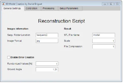
Once this is done a window like shown below will pop up showing multiple tabs. In the general settings tab it is possible to set the name of the folder where the sequence is stored as well as the image type (png, jpg…). On the right of the following figure the name of the final STL file can be set with the compression factor of this file. If the dimension of the item should be change the scale value can be changed.

For testing purpose there is also the possibility to create some errors in the matrix used to make the reconstruction. One possibility is to randomize values in the matrix and the other way is to give the

ground a slop. Ideally even with this activated there should be no change in the resulting model because the error correction is implemented.

6.2.2 Calibration

The next tab lets the user select between the two calibration methods. One is based on a picture taken with known dimension and the other with information from the sensor datasheet used in the camera. More details on how the calibration works can be found in the next chapter.

6.2.3 Processing

Coming to the processing tab the user can change the way the image is processed. This tab is the most important one when it comes to influence the quality of the resulting model.

With the different parameters the way some function works can be changed. The limiter has two option, but it is recommended to keep the ponderation value small so that the area value can be more important resulting in better result. If there are a lot of small dots from reflected light on the image the “Finder Min Object Size” can be increased.

Figure 17: GUI general settings tab

The values under “Height” are used to define the ground position on the image. But the most important factor is the smooth one under “Matrix Processing”. Like its name implies it will smoothen out the surface of the model. This value needs to be used with moderation.

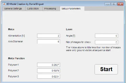
6.2.4 Setup parameters

After the processing tab comes the final tab called “Setup Parameters”. In this tab the values set depend on how the system was mounted. For example the motor alimentation and the polynomial function to determine the speed when the item was pulled. The measurement to define this function with the current motor can be found in the appendix.

To determine the laser rotation angle on images a number of pictures is checked. This specific amount can be set here. This number should be little less than the number of pictures at start of scan where only the ground line can be seen.

Like explained before the laser needs to hit the item with an angle. This value is used to calculate the item. The reconstruction is lunched by pressing the start button. In the Matlab command window the user can control the program status.

Figure 19: GUI processing tab

7 Implementations

The following chapter explains more precisely how the program works behind the GUI after pressing the start button. It clarifies each function executed during the modelisation. There are also examples in this chapter about the different functionalities implemented.

7.1 Calibration

The first step is to create a relationship between the model and the real object. This is achieved by making a calibration. Like mentioned once before there are two possible ways this can be done. One way is to take a picture of a checkerboard pattern with squares of known dimensions 𝑙 [𝑚𝑚]. Then the image is processed by measuring the average square length 𝑝 [𝑝𝑥] on the image. The factor 𝑓 [𝑚𝑚/𝑝𝑥] between the known dimensions and the number of pixels allows to calculate the item width.

𝑓 = 𝑙 𝑝

The other way would be to use the pixel size 𝑝𝑠 [𝑚𝑚/𝑝𝑥] given in the datasheet from the camera sensor. The reason why 𝑓 = 𝑝𝑠 is because of the use of the telecentric lens. Other information from the datasheet that can be help calculate the pixel size are the image size 𝑖𝑠 [𝑚𝑚] and number of pixels 𝑛𝑝 [𝑝𝑥].

𝑝𝑠 = 𝑖𝑠 𝑛𝑝

7.2 Factory

After successfully getting the relation between px and mm the factory function is called. This is the most important function that is executed and takes around 95% from the whole processing time. The factory returns a 2D matrix holding values used to calculate the height of every point from the object. Most of the settings in the reconstruction script are passed down to this function.

7.2.1 Removing images

Before processing any images all the pictures where no line can be found are removed from the directory. Same goes for images where the line is only partially visible. This will prevent to waste time trying to process images that will give no relevant result anyway. This part of the function only removes pictures at the start of sequence. This prevents from losing pictures in the middle of scan used to determine the item length.

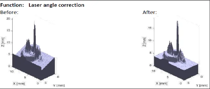
7.2.2 Laser angle correction

The next step in the factory is rotating the image if necessary. Because the laser is mounted in a flexible fashion it is possible that the line on the image is not perfectly horizontal. When starting a scan some pictures from the ground are obligatory taken. The ground that is flat will not deform the line and should return a horizontal line. If this is not the case some correction can be done, by calculating the angle of the line amongst the first few pictures of the sequence. Then all following images are rotated accordingly by the determinate angle before further processing.

This also has some interesting “side effect” visualized with figure below. When rotating the image instead of trimming the image back to its original dimensions, padding is added to preserve the line length. Because of the angle the line is longer than it would be if it was horizontal. Making it possible to scan larger items. Thought for it to work well, the items still needs to move perpendicular to the laser line. Another problem when trying to exploit this is the fact that some height is lost, the item can’t be that huge on the extremities of the line.

The figure below shows what the model would look like with and without the laser angle correction. Other corrections are excluded as well so that a flow of progess amongst the next few figures with “before/after” can be recognized.

Figure 23: Model before and after angle correction

The ground position on the image is now defined for later use. For this only the first few images are used once more.

Figure 21: Image rotation flow

Figure 22: Image line growing size

7.2.3 Processing Images

Now that the image is rotated correctly the first step to build the 3D model is detecting the line position on the different images.

To be able to differentiate between anything else on the image and the line, the image needs to be converted to a logical map. In a first step this is achieved by converting the pictures to grayscale because the images stored by the camera are in RGB format. Even if a monochrome camera is used the image are stored as RGB format. But now the image only consists of a 2D matrix with cells going from 0 to 255. The figure below shows what the line looks like after the conversion.

Next step is to convert matrix to a binaries map. All cells below a certain values are set to 0 and the rest to 1. It’s like setting the contrast to maximum. Now the image is only black & white. The image now looks like the figure shown below.

Afterwards the map is cut into strips. The strips are 1 column large representing precisely one column of pixels from the base image. On the strips the line positions is detected with the “finder” function explained further below. This can be done because the line is marked as ones on the strips after all the conversions executed before. The position on the strip is the coordinate of a point from the line on the image. Every strip can only have 1 position, but it is possible that it does not have any as well. For example, if the contrast setting is to low, it happens that not all points were found. Thus, data is lost. The table below shows how the matrix is structured in which those position are stored. The columns represent on what image the position was found and row what strip of said image it was.

image001 image002 image003 image004 image005

strip001 - - - - -

strip002 - - - - -

strip003 - - - - -

strip004 - - - - -

strip005 - - - - -

Table 2: How images and strips are sorted in matrix

7.2.4 Finder

To detect object in a binary map there already exists a function in Matlab called “regionprops”. This function would look for a group of 1 in a matrix. Then the function could return the position, size, boundary and so on of this object. The function was also used to find object on strip. But because of the amount of strips it slowed down the processing time drastically. This is why this function was developed. The Matlab function is still used to find objects when correcting the laser angle. Before the regionprops took 390s to process a sequence with the new function it only took 41s to process the same sequence.

Figure 24: Grayscale image of laser line

The main reason to be able to improve the speed is the limitation of strip size to 1. This way only arrays need to be processed and not a matrix like regionprops can do.

The finder takes a sequence of numbers consisting only of ones and zeros. In the case of this project it is given column after column coming from the logical map. This function looks for the longest sequence of ones in the column. Then it returns the centre position in the array of this sequence.

0 1 1 0 0 1 1 1 1 1 0 0 1

Table 3: Finder locating centre in array

The table above shows an example of the array. In grey is marked the longest sequence of ones found. The position returned is 8 because that’s where the centre of the queue of ones is located in the sequence. If multiple sequences have the same size the first one found is returned. It would be possible to return NaN so that the error correction will fill the spot. The problem with that is the fact that there are already enough points missing and after some testing the result are better when keeping this points and removing it later if the value is not coherent.

7.2.5 Limiter

Like mentioned just now the next step executed by the factory is to remove non-coherent values in the matrix. Those spices (positive/negative) can appear when the laser reflected on a metallic part and can be seen on the image at a random position. To remove such values the limiter function is called. The limiter function checks if there is an important change in height with a point in the matrix and the adjacent values. The importance of this change can be set with a parameter. A huge change in value is justified if enough points in an area also have approximately the same value. Those two criteria allows to detect spices in the matrix.

The figure below shows the value 9 in the matrix is not coherent ant the limiter replaces it with NaN.

A spice value is removed when detected. But not all spices are detected the first time when the limiter is executed. Therefore, the limiter is a recursive function. It removes all spices until there are no new ones found. In case that every time the function is called only a few values are removed there is a counter to limit the recursions. This way the program doesn’t get stuck in a loop for too long. Because if only a few points change the modification on the result are minimal. Finally a median filter is applied for good measure. The filter is a function from Matlab and will do minor changes to the matrix.

Below can be seen a figure representing the further model development with this function correcting the data.

Figure 27: Model before and after limiter function

7.2.6 Filling missing data

Removing spices values, having to high of a contrast setting and sometimes just having the line on the image hidden for some reason, all this can create missing data in the matrix.

These missing digits need to be padded. There are multiple ways to do it resulting in different values stored. One way is to just imitate the nearest existing value. Another possibility is to make a linear connection between multiple adjacent known cells from the matrix. Example what this look like is given with the next two tables.

Before 1 2 NaN NaN 5 After 1 2 3 4 5 Table 4: Filling missing data with “linear” method

Before 1 2 NaN NaN 5 After 1 2 2 5 5

Table 5: Filling missing data with “nearest” method

The ground position defined earlier is now used to invert the data in the matrix. If the average value of the matrix is less than the ground value it means the images would have needed to be rotated by 180°, but to simplify this for the user it is detected this way.

7.2.7 Smooth

Now that there is a matrix full of values and data a smooth function is applied for cosmetic purpose on the model. If the smooth factor is too big it will falsify the model and start “merging” the model to the ground. But a little smoothing the panel helps to have cleaner surface and flatten out smaller spices.

7.2.8 Ground angle correction

The function called “ground_balancer” executed in the factory looks for a height difference between the ground at start and end of scan. The reason this is needed is if the ground is not perfectly levelled. By comparing the ground height at start and end of scan the height difference can be defined and the values in the matrix can be corrected with the slop accordingly. The following figure shows what this would look like. On the left the ground was artificially changed and the correction deactivated to make it clearer.

Figure 28: Model before and after ground_balancer function

7.2.9 Pull model down to ground

The last step which changes the values in the matrix is the following part of the factory. If the laser hits the carriage and on the image the line is in the centre, this means the ground for the model doesn’t start at 0 but at the centre (position in image).

Because the ground was levelled in the previous function the value originally stored from the images can’t be used anymore. To find the new ground the average value in the first column from the matrix is used.

After finding that value the entire matrix subtracted by it. Negative values are corrected to 0 and the result can be seen in the figure below.

Figure 29: Model before and after setting ground to value 0 in matrix

7.2.10 Cutter

After this step there is no use for the ground anymore. The goal here is to remove rows and columns from the matrix with no relevant values about the item. This way the matrix is trimmed to only hold values coming from images where the item was on it.

A specific value is used to determin because the ground is not perfectly smooth. This value is used as a limit. The matrix is trimmed starting from outsides to inside. Every row or column not having a value higher than the limit is removed.

This function will stop removing columns from one side if it found a value higher than the ground limit, like hitting a wall. This is done by going through the matrix and storing the positions of the first row and column holding a value higher than the ground limit. Same is done by storing the row and column holding the last value above the limit. Then the matrix is trimmed to those rows and columns, giving it new dimensions and removing all excessive ground around the item.

This marks the end of the factory function and the figure below shows the resulting model. Now the factory returns the matrix holding all those values.

Figure 30: Model before and after cutting matrix border

7.3 Dimension corrections

After getting the matrix (z) holding all the values from the scanned item, 2 more matrixes are created. One matrix is the matrix (x) giving the width of the item and the last one is the matrix (y) giving the length of the object.

7.3.1 Width

The width can be found out by counting the amount of rows from the z matrix representing the strips of 1 pixel width. The conversion from the number of pixel to mm can be done thanks to the calibration done at the beginning of the reconstruction function. The value found is stored in the y matrix by filling the every column linearly from 0 to this value. The y matrix would look similar to the following table, but there is still the need to calculate the length and the model height.

0 0 0 1 1 1 2 2 2

Table 6: How y matrix is filled

7.3.2 Height

To calculate the height out from the values stored in the z matrix those values need to be converted. The values stored are the length difference between where the laser hits on and the ground and the laser hits the item. To calculate the height the angle between the laser and the lens is needed.

In the first figure below the value 𝑙 represents the value stored in the z matrix being the length difference. The red lines are the laser line on the image.

Then when knowing the length 𝑙 and the angle (α) the height (h) can be calculated thanks to trigonometry. The figure below shows the triangle and the different parameters needed. Now with the function ℎ =_{tan (𝛼)}𝑙 the height is calculated. But like with the width the height value is in pixel. To convert the data to mm the same method with the calibration is applied.

7.3.3 Length

Now for the reconstruction function to calculate the length, it is necessary to know at what speed the item was moving forward. Thanks to the function giving the motor rpm passed down from the GUI this can be calculated. Once this is known and the camera framerate is also given by the GUI. By just counting the number of pictures (columns of matrix) the camera took from the item and multiplying it by the motor speed it returns the item length.

Then something similar is done as before when creating the width matrix. Now the value found is stored in the x matrix by filling the every row linearly from 0 to item length. The x matrix also looks similar to the previous table but with a small but important difference. Like shown in the table below. Another important condition is for the x and y matrices to have the same dimension as the z matrix. This is needed for the final step.

0 1 2 0 1 2 0 1 2

Table 7: How x matrix is filled Figure 31: Length l from

line deformation

Figure 32: Trigonometry visualisation to

7.4 STL file

After creating all the matrices the goal is the STL file creation. Being one of the most common format for a 3D model this file can be visualized in most programs. To create the model the 3 matrices created are combined to build a patch model holding the vertices and faces of the scanned item. This is done by a script found on the Matlab forum called “surf2solid”. This script was provided by Sven Holcombe. Next if the user decided to change the model scale, the vertices are multiplied by given factor. Then the STL file is created by giving the patch as parameter to a function called “stlwrite”. This function has the same author as the surf2solid function.

8 Tests & Results

To do the testing of the whole setup a hexagonal nut was scanned multiple times. The specific parameter used for the GUI can be found in the “workspace_test_settings” file. This file can be loaded into the Matlab workspace. After every scan the STL file was visualized with “Autodesk Inventor Professional 2019” and then the measurement were taken on the model. The file with all the resulting measurements can be found in the appendix.

8.1 Item scans

The test item was a M2.5 hexagonal nut (BN109). The item blueprint is shown in the figure below with 2 different point of view.

The values for the different dimension can be found in the following table. Unfortunatly the dimension D and D2 were ignored during the measurments because of the strong reflection of the metalic surface in the hole of the nut. The hole of the models were definitly not accurate enough to be considerd.

Dimension name Distance [mm]

E 5.45

S 5

M 2

D 2.5

D2 4.1

Table 8: Dimensions value to blueprint of nut

The following two figures shows examples of such scans. The item was scanned 20 times. On the figure located to the right where the nut is seen from above, the line, where there is some rounding on the edges, can slightly be seen.

Figure 33: Nut blueprint Source: Bossard, BN109, ref. 1088254

Because the upper surface of the item is not flat the M measurements were taken at 2 different places for each model. Once at the highest point of the profile from said model (upper M) and once at the lowest point of the surface (lower M). This would result in giving information about the height range of each model.

For each type of measurement taken a histogram has been done, showing in what range most of the measurements are.

Figure 36: Histogram on distance from ground to upper height limit

The figure above shows where most of the upper M measurement were. The real M dimension is 2mm, this means the majority of those measurement are in a 0.22 offset range from correct distance. Average distance measured is 2.173mm giving on average a 0.173mm difference.

Figure 37: Histogram on distance from ground to lower height limit

The next figure visualises the lower M measurements. The offset range here is slightly larger and there average difference to the real item is 0.175mm lower than it.

Figure 38: Histogram on distance from nut sides

The highest difference measured in the upper M is 0.37mm and the max difference with the lower M is 0.475mm. The total average height is little lower than the real item and the average tolerance is ±0.174mm.

Here above can be seen the histogram on the S size. The correct distance is at 5mm. As can be seen on the histogram most of the data is lower than those 5mm. The range of for the S is +0.13mm and -0.073mm with an average tolerance of ±0.103

The histogram below shows the E measurements taken. The real size would be 5.45mm but once again most of the measurements are lower than that. For the E dimension the range of data is between +0.293mm and -0.523mm. Those 0.523mm is the highest difference found with the actual size. On average the tolerance for the edge is ±0.084.

Figure 39: Histogram on dimensions from nut edge

The reasons the S and E dimensions are distorted is due to multiple elements. But this is a constant offset that can be corrected by changing the parameters done to the GUI. More details to those distortion sources are mentioned in the next chapter.

8.2 Error Sources

Some difference between the real object and the model appear because the line projected by the laser is not always perfectly continues, as well as the fact that when filling missing data in the matrix is just an approximate correction but doesn’t have to be true. Below are mentioned the factor creating errors especially in the x (length), y (width) and z direction. The error coming on the S and E measurement from the previous chapter are both heavily influences by the errors coming from the width and length error sources.

8.2.1 Length

Some length of the object can be lost if for example the camera doesn’t take the picture exactly when the laser hits the item border at start of scan. Meaning the item will move under the laser in between two frames of the camera. Same goes for the end of scan. In those two cases frames where the item could have been seen are missing.

Another reason the length is wrong is because the calculated motor movement speed is not perfectly correct. This is due to some small difference when calculating the rpm with data from the GUI and the actual motor rpm. Then this difference is multiplied by a factor when converting the rpm to the movement speed.

8.2.2 Width

There are two reasons that can make the width measurement go wrong. This depending on what calibration method was used. This error will also add up to the height error source because it also uses the calibration to convert the values stored in pixel unit to mm.

When using the checkerboard method to make the calibration some error appears already when printing the checkerboard. The next reason is that when taking a picture of the checkerboard the image will not have perfect contrast. Those two reasons will create some error when counting the number of pixels a

square from the checkerboard has. This value with error is then used to calculate the relation between pixels and mm in the calibration procedure.

Therefore, the better choice for the calibration is to use the parameters of the camera given in the datasheet. Especially since that information can be used without problem thanks to the telecentric lens. The only factors creating error here is the slightly fuzzy image when the image is out of focus and the fact that there is not an ideal telecentric lens perfectly negating the depth perception.

8.2.3 Height

The major reason why there is a difference in height is the angle setting in the GUI. Currently the way the system is set up makes it difficult to determine the laser angle. To resolve this problem once the laser is set up it is recommended to scan an item of known height and then set the angle parameter in a way that the model reconstructed correspond to the real item.

8.3 Unknown

Sometimes there is also some unknown error occurring. This strange behaviour doesn’t happened directly on the item and doesn’t influences its dimension but it’s more like there is a problem occurring somewhere and filling the matrix on its extremities with strange values. This prevents the cutter function to work properly. The figure below shows an example of such an occurrence.

Figure 40: Model of unknown error occurring

8.4 Randomized

Now that most problems have been considered it would be interesting to test the limit of the software. To achieve this a function was implemented that can randomize a percentage of cells from the z matrix used during the reconstruction. The values are randomized before any correction is applied on the matrix.

The next two figures show the model when 0% and 10% of the matrix is randomized. The right figure is still accurate but first changes can be observed. In general the surface of the model appears smoother. This is probably because the limiter is removing more values, resulting in further data missing and that needs to be artificially filled in.

The next two figures below show the model with 20% and 30% randomized matrices. In the left matrix important changes are happening on the model. It seems like some part in the centre (on y axe) of the model is starting to miss too much data. Those places seem like a weak spot of the scan. Those places where more data is missing in the matrix is where on the image a lot of reflection can be found. This means that previously the limiter already removed a lot of values there and now with the randomizing even more is removed. On the right side the image with 30% randomized the item is nearly cut in half at those weak points.

Figure 41: Model 0% randomized values Figure 42: Model 10% randomized values

9 Future improvements

After having figured out most information on the system there are still further possibility to improve the prototype. Most improvements, with significant impact on the model quality, that can be done are hardware sided, there is only so much that can be fixed with the software. The next points will discuss the possible amelioration the system can undergo. Some of these changes would improve the existing results and other would be pretty big changes that would need a complete rework of the current setup.

9.1 Multi-profile

The huge change that would require to rework most of the current setup is the following one.

In the current state the system only scans one item profile at the time. Also because of the laser brightness no colour filter is necessary (originally planned to use one). What could be done is mounting more cameras, as well as filters of different colours and corresponding lasers, on the system. This would allow to simultaneously scan 3 profiles. Right now, if 3 profiles from the same item want to be reconstructed, it is necessary to perform 3 scans, resulting in 3 different models. But if the scans are made simultaneously it would save time and under the condition that the lasers are perfectly aligned on the model, the creation of 1 model with all 3 profiles can be achieved. Meaning there will also be a need to make major changes in the software to be able to manage that.

9.2 Conveyer

Another upgrade would be to change from a motor pulling the item to build a real conveyer belt. Allowing to have a much smoother and constant progressing item movement under the lens. A stepper motor could be used to move the conveyer. The motor in return is commanded by a module or some software combined with Matlab running on the PC. This way when the user presses the start button in the GUI a scan is automatically started and processed.

Figure 45: Laser of different colours on same item but different

9.3 Laser

Because the scan quality strongly depends on the laser there are also some improvements to be done here. Using a different approach to direct the laser on the item would help removing missing laser lane in some images. For example, having multiple laser creating the same line from different positions but with the same angle to the lens. The figure below shows such an example where some line is missing on the image.

Another way to improve would be to take a laser with less power avoiding some reflection on metallic surfaces as well as using a laser with better focus resulting in thinner line on the image.

9.4 Camera/Lens

The following is to consider when trying to improve the resolution of the model by changing camera and/or lens, for example installing a bigger lens to scan a larger item.

Taking a lens with magnification lower than 1 will result in a larger field of view. But if only that field of view is increased, and the pixel amount on the image is the same there will be a loss in resolution. To counter that it would be appropriate to take a sensor who also has more pixels. The more pixel the image at the end has the more slices can be cut, getting more details for the model.

9.5 User friendly

On the software there is always something to improve or that can be tweak around. But one of the most important would be to make the GUI more user friendly. Currently there are a lot of parameters that need to be set. The goal here would be to find ways to reduce the amount of variable or even limit those who are not used often.

9.6 Recursive laser correction

Another modification that can be done to upgrade the software further is making the function that is responsible for checking the laser rotation angle recursive. This way the function will balance out the image till the laser is “horizontal”, like this the function will work in a similar to the already existing recursive function “ground_balancer”.

10 Conclusion

This thesis was about developing a 3D scanner capable of reconstruction items in motion. This goal has been fulfilled. Right now, the prototype allows to scan items that are 7mm wide, 3 mm height and there is no length limitation.

Thanks to the tests, it can be conclude that the system has a height resolution of 0.1mm. Meaning engravings of 0.1mm depth can be seen, but this depends on the laser angle settings. The range difference between model and item goes from 0.523mm under the real dimension to 0.370mm above it. The average height tolerance is ±0.174mm and on the sides it is ±0.094mm. For the item to be scanned a minimal height of 0.3mm is required but this value is difficult to define when the tolerance range of the system is larger than that.

There is also a constant offset in the average dimension measured compared to the real item dimensions. The main reason for this, is the way the system is built. When designing the prototype the goal was to provide as many possibilities as possible that would allow an adaptive setup. For example being able to change the lens used, changing the laser angle or modifying the direction the laser comes from. All of those flexible parameters make it difficult to define the right settings needs by the GUI.

Even if this marks the end of the bachelor thesis, there are always improvement that can be done. For example to improve the system significantly, hardware that can be set more accurately, is required. Thought the biggest obstacle with this is, that the whole system gets quickly very expensive. Currently only for the prototype the material and components used are worth 1652.20 CHF, the detailed budget plan can be found in the appendix.

………. Daniel Briguet, Sion the 17.08.2018

11 Credits

Special thanks to the following people for helping me realize this project: • Djano Kandaswamy, responsible professor, HEVs

• Bernard Loehr, expert, HE-ARC

• Jonathan Michel, student & colleague, HEVs • Joost Laros, student & colleague, HEVs

• Sven Holcombe, author of “surf2solid.m” and “stlwrite.m” Matlab scripts

12 Bibliography

EDMUND OPTICS, The Advantages of Telecentricity, https://www.edmundoptics.com/resources/application-

notes/imaging/advantages-of-telecentricity/, (Consulted the 11.06.2018)

EDMUND OPTICS, Telecentric Design Topics, https://www.edmundoptics.com/resources/application-

notes/imaging/telecentric-design-topics/, (Consulted the 11.06.2018)

APTINA, CMOS Digital Image Sensor,

https://s1-dl.theimagingsource.com/api/2.5/packages/publications/sensors-cmos/mt9p031/bf1d60cb-e460-5c33-a560-a6e26b5def56/mt9p031_1.2.en_US.pdf, (Consulted the 11.06.2018)

13 List of Figures

FIGURE 1: LEFT LASER PROJECTED ON ITEM. RIGHT LASER LINE SEEN FROM ABOVE ... 3 FIGURE 2: PICTURE THROUGH DIFFERENT LENSES, LEFT STANDARD AND RIGHT TELECENTRIC ... 4 FIGURE 3: LIGHT RAYS AT AN OBJECT TELECENTRIC LENS ... 4 FIGURE 4: LIGHT RAYS WITH AN IMAGE TELECENTRIC LENS ... 5 FIGURE 5: COMPARISON GRAPH BETWEEN THE DIFFERENT LENSES ... 5 FIGURE 6: PROTOTYPE SYSTEM SETUP ... 6 FIGURE 7: IMAGE OF LASER REFLECTION ON METALLIC PART ... 8 FIGURE 8: LASER LINE WITH VARIOUS SETTING ... 8 FIGURE 9: SIDE VIEW FROM LASER AND LENS UNTO THE OBJECT ... 9 FIGURE 10: SIDE VIEW OF LASER GOING PAST OBJECT ... 9 FIGURE 11: VIEW FROM FRONT WHEN LASER HITS OBJECT FROM ABOVE BUT NOT ON THE SIDES ... 10 FIGURE 12: LASER NOT REACHING HOLE GROUND ... 10 FIGURE 13: LASER GOING UNDERNEATH OBJECT... 11 FIGURE 14: CONVERSION STEP DIAGRAM FROM IMAGES TO 3D MODEL ... 12 FIGURE 15: SOFTWARE CLASS DIAGRAM ... 13 FIGURE 16: SOFTWARE FLOWCHART ... 13 FIGURE 17: GUI GENERAL SETTINGS TAB ... 16 FIGURE 18: GUI CALIBRATION TAB... 16 FIGURE 19: GUI PROCESSING TAB ... 17 FIGURE 20: GUI SETUP PARAMETERS TAB ... 17 FIGURE 21: IMAGE ROTATION FLOW ... 19

FIGURE 22: IMAGE LINE GROWING SIZE WHEN LEVELLED ... 19 FIGURE 23: MODEL BEFORE AND AFTER ANGLE CORRECTION ... 19 FIGURE 24: GRAYSCALE IMAGE OF LASER LINE ... 20 FIGURE 25: BINARY IMAGE OF LASER LINE ... 20 FIGURE 26: LEFT MATRIX BEFORE LIMITER AND RIGHT MATRIX AFTER LIMITER ... 21 FIGURE 27: MODEL BEFORE AND AFTER LIMITER FUNCTION ... 22 FIGURE 28: MODEL BEFORE AND AFTER GROUND_BALANCER FUNCTION ... 23 FIGURE 29: MODEL BEFORE AND AFTER SETTING GROUND TO VALUE 0 IN MATRIX ... 23 FIGURE 30: MODEL BEFORE AND AFTER CUTTING MATRIX BORDER ... 24 FIGURE 31: LENGTH L FROM LINE DEFORMATION ... 25 FIGURE 32: TRIGONOMETRY VISUALISATION TO CONVERT LENGTH FROM GROUND TO HEIGHT ... 25 FIGURE 33: NUT BLUEPRINT ... 27 FIGURE 34: TEST ITEM MODEL ... 28 FIGURE 35: TEST ITEM FROM ABOVE ... 28 FIGURE 36: HISTOGRAM ON DISTANCE FROM GROUND TO UPPER HEIGHT LIMIT ... 28 FIGURE 37: HISTOGRAM ON DISTANCE FROM GROUND TO LOWER HEIGHT LIMIT ... 29 FIGURE 38: HISTOGRAM ON DISTANCE FROM NUT SIDES ... 29 FIGURE 39: HISTOGRAM ON DIMENSIONS FROM NUT EDGE ... 30 FIGURE 40: MODEL OF UNKNOWN ERROR OCCURRING ... 31 FIGURE 41: MODEL 0% RANDOMIZED VALUES ... 32 FIGURE 42: MODEL 10% RANDOMIZED VALUES ... 32 FIGURE 43: MODEL 20% RANDOMIZED VALUES ... 32 FIGURE 44: MODEL 30% RANDOMIZED VALUES ... 32 FIGURE 45: LASER OF DIFFERENT COLOURS ON SAME ITEM BUT DIFFERENT PROFILES ... 33 FIGURE 46: IMAGE OF LASER LINE WITH SOME MISSING ITEM BORDER ... 34

14 List of tables

TABLE 1: REQUIRED ADD-ONS FOR SCRIPTS ... 12 TABLE 2: HOW IMAGES AND STRIPS ARE SORTED IN MATRIX ... 20 TABLE 3: FINDER LOCATING CENTRE IN ARRAY ... 21 TABLE 4: FILLING MISSING DATA WITH “LINEAR” METHOD ... 22 TABLE 5: FILLING MISSING DATA WITH “NEAREST” METHOD ... 22 TABLE 6: HOW Y MATRIX IS FILLED ... 24 TABLE 7: HOW X MATRIX IS FILLED ... 25 TABLE 8: DIMENSIONS VALUE TO BLUEPRINT OF NUT ... 27

15 Appendix

• Appendix1 Lens selection procedure

• Appendix2 Motor measurements for function

• Appendix3 Measurements done for test & result chapter • Appendix4 Budget

• Appendix5 Hardware blueprints • Appendix6 Laser information • Appendix7 Motor datasheet • Appendix8 Lens datasheet • Appendix9 Camera blueprint

Appendix 1

X Magnification 0.2 0.151 0.184 1 0.5 1 3 2 2 1 1 2 1 2 2 4 8 0.75 4 4 0.75 3

mm Field of View 1/2 32 42.4 34.7 6.4 12.8 6.4 2.1 3.2 3.2 6.4 6.4 3.2 6.4 3.2 3.2 1.6 0.8 8.5 1.6 1.6 8.5 19

Euro Price 995 1495 1495 525 895 725 575 995 575 525 525 725 725 550 550 595 675 895 1250 595 625 7

Yes(1)/No(0) Double Sided Telecentric 1 0 0 0 1 0 0 1 0 0 0 0 0 0 0 0 0 1 1 0 0 16

mm Working Distance 164 111 110 40 120 220 40 75 110 65 110 300 300 40 65 40 65 100 44 65 110 17

±mm Working Distance Tolerance 3 0 0 1 3 2 1 3 1 1 1 2 2 1 1 1 1 3 3 1 1 20 22 giving ponderation and dividing by av. giving then ranking

Unit Criteria Model 1 Model 2 Model 3 Model 4 Model 5 Model 6 Model 7 Model 8 Model 9 Model 10 Model 11 Model 12 Model 13 Model 14 Model 15 Model 16 Model 17 Model 18 Model 19 Model 20 Model 21 Model 22 Average Ponderation Hiden Model

±mm Depth of Field 12.9 0.5 2.1 0.6 0.13 0.49 0.9 1.2 0.3 0.4 0.17 0.23 0.8 1.2 1.57 8 13

X Magnification 0.2 1 0.5 1 2 2 1 1 2 1 2 2 0.75 0.75 1.23 7 12

mm Field of View 1/2 32 6.4 12.8 6.4 3.2 3.2 6.4 6.4 3.2 6.4 3.2 3.2 8.5 8.5 7.84 6 6

Euro Price 995 525 895 725 995 575 525 525 725 725 550 550 895 625 702.14 5 4

Yes(1)/No(0) Double Sided Telecentric 1 0 1 0 1 0 0 0 0 0 0 0 1 0 0.29 2

mm Working Distance 164 40 120 220 75 110 65 110 300 300 40 65 100 110 129.93 1

±mm Working Distance Tolerance 3 1 3 2 3 1 1 1 2 2 1 1 3 1 1.79 1 Result 91.87 9.66 24.75 7.92 15.52 11.97 11.51 12.70 9.02 6.29 11.05 11.16 16.40 12.17

filtering by some min and max values

Unit Criteria Model 1 Model 2 Model 3 Model 4 Model 5 Model 6 Model 7 Model 8 Model 9 Model 10 Model 11 Model 12 Model 13 Model 14 Model 15 Model 16 Model 17 Model 18 Model 19 Model 20 Model 21 Model 22 Hiden Model

±mm Depth of Field 12.9 2.1 0.13 0.49 0.9 1.2 0.17 0.23 0.8 1.2 min of 0.4mm 8

X Magnification 0.2 0.5 2 2 1 1 2 2 0.75 0.75 min 0.5 X 14

mm Field of View 1/2 32 12.8 3.2 3.2 6.4 6.4 3.2 3.2 8.5 8.5 min 6 mm 15

Euro Price 995 895 995 575 525 525 550 550 895 625 max 1k 1

Yes(1)/No(0) Double Sided Telecentric 1 1 1 0 0 0 0 0 1 0 don't care 9

mm Working Distance 164 120 75 110 65 110 40 65 100 110 don't care

±mm Working Distance Tolerance 3 3 3 1 1 1 1 1 3 1 don't care ponderation but using median val as divider

Unit Criteria Model 1 Model 2 Model 3 Model 4 Model 5 Model 6 Model 7 Model 8 Model 9 Model 10 Model 11 Model 12 Model 13 Model 14 Model 15 Model 16 Model 17 Model 18 Model 19 Model 20 Model 21 Model 22 median Ponderation Hiden Model

±mm Depth of Field 2.1 0.9 1.2 0.8 1.2 1.20 8 18

X Magnification 0.5 1 1 0.75 0.75 0.75 7 10

mm Field of View 1/2 12.8 6.4 6.4 8.5 8.5 8.50 6

Euro Price 895 525 525 895 625 625.00 5

Yes(1)/No(0) Double Sided Telecentric 1 0 0 1 0 99999.00 2 median is 0 not good

mm Working Distance 120 65 110 100 110 110.00 1

±mm Working Distance Tolerance 3 1 1 3 1 1.00 1 Result 22.45 16.06 17.65 13.26 16.00

Appendix 2

2.00 1.60 4.00 3.00 6.00 4.60 8.00 6.40 y = 0.025x2_{+ 0.55x + 0.4} 0 2 4 6 8 10 12 0 2 4 6 8 10 12 rp m [V]

Appendix 3

2 2.14 1.76 4.69 5.29 3 2.30 1.90 4.70 5.31 4 2.37 1.53 4.71 5.44 5 2.27 1.81 4.59 5.17 6 2.07 1.79 4.68 5.48 7 2.12 1.69 4.66 5.09 8 2.28 1.76 4.70 5.30 9 2.09 1.78 4.81 5.06 10 2.15 1.69 4.84 5.20 11 2.19 1.99 4.90 4.93 12 2.18 1.86 4.92 5.13 13 2.16 1.94 5.13 5.74 14 2.21 1.97 4.82 5.33 15 2.14 1.94 5.01 5.23 16 2.11 1.86 4.89 5.33 17 2.07 1.84 4.78 5.38 18 2.14 1.91 5.12 5.51 19 2.16 1.78 4.75 5.38 20 2.12 1.91 4.72 5.16

Appendix 4