Scalpel-CD
: Leveraging Crowdsourcing and Deep Probabilistic
Modeling for Debugging Noisy Training Data
Jie Yang
University of Fribourg Fribourg, Switzerland [email protected]Alisa Smirnova
University of Fribourg Fribourg, Switzerland [email protected]Dingqi Yang
University of Fribourg Fribourg, Switzerland [email protected]Gianluca Demartini
University of Queensland St Lucia, Australia [email protected]Yuan Lu
ING Domestic Bank Nederland Amsterdam, Netherlands [email protected]
Philippe Cudré-Mauroux
University of Fribourg Fribourg, Switzerland [email protected]ABSTRACT
This paper presents Scalpel-CD, a first-of-its-kind system that leverages both human and machine intelligence to debug noisy labels from the training data of machine learning systems. Our system identifies potentially wrong labels using a deep probabilistic model, which is able to infer the latent class of a high-dimensional data instance by exploiting data distributions in the underlying latent feature space. To minimize crowd efforts, it employs a data sampler which selects data instances that would benefit the most from being inspected by the crowd. The manually verified labels are then propagated to similar data instances in the original training data by exploiting the underlying data structure, thus scaling out the contribution from the crowd. Scalpel-CD is designed with a set of algorithmic solutions to automatically search for the optimal configurations for different types of training data, in terms of the underlying data structure, noise ratio, and noise types (random vs. structural). In a real deployment on multiple machine learning tasks, we demonstrate that Scalpel-CD is able to improve label quality by 12.9% with only 2.8% instances inspected by the crowd.
CCS CONCEPTS
• Information systems → Crowdsourcing; • Computing methodologies → Neural networks; Latent variable models.
KEYWORDS
Debugging training data; crowdsourcing; deep probabilistic models ACM Reference Format:
Jie Yang, Alisa Smirnova, Dingqi Yang, Gianluca Demartini, Yuan Lu, and Philippe Cudré-Mauroux. 2019. Scalpel-CD: Leveraging Crowdsourcing and Deep Probabilistic Modeling for Debugging Noisy Training Data. In Proceedings of the 2019 World Wide Web Conference (WWW ’19), May 13–17, 2019, San Francisco, CA, USA. ACM, New York, NY, USA, 11 pages. https://doi.org/10.1145/3308558.3313599
This paper is published under the Creative Commons Attribution 4.0 International (CC-BY 4.0) license. Authors reserve their rights to disseminate the work on their personal and corporate Web sites with the appropriate attribution.
WWW ’19, May 13–17, 2019, San Francisco, CA, USA
© 2019 IW3C2 (International World Wide Web Conference Committee), published under Creative Commons CC-BY 4.0 License.
ACM ISBN 978-1-4503-6674-8/19/05. https://doi.org/10.1145/3308558.3313599
1
INTRODUCTION
The success of machine learning techniques — deep learning in particular — heavily relies on the quality and quantity of labeled training data [49]. While a growing body of research has addressed the data quantity issue [2, 9, 15, 31, 47], relatively little work has been focused on the data quality issue. Due to the lack of trans-parency and accountability of deep learning models [11, 19, 25], incorrect labels in the training data are generally difficult to iden-tify when the prediction goes wrong; consequently, label noise has become a main obstacle for developing, deploying, and improv-ing deep learnimprov-ing models. The significance of the problem is more obvious in critical domains such as health or justice [34]. For in-stance, in a medical context, models trained on drug instances that are wrongly labeled as successfully treating a certain condition would likely produce erroneous and damaging effects. We therefore argue that debugging noisy labels is of key importance for deep learning-based systems, both in terms of performance and security. The main existing approach in that context leverages data tributions for debugging noisy labels (see Section 5 for more dis-cussion on that point). The basic assumption is that data points distributed close to each other are more likely to have the same label. Existing methods [1, 35, 39], however, suffer from two major limitations. First, they only model data distributions in the low-level feature space with oversimplified structures (e.g., bag-of-words). As for most language and vision problems, the low-level distribu-tions learned by these methods are limited compared to the true distributions that present complex dependencies among features. The second limitation, perhaps the most important one, is that all existing methods are automatic methods that rely on machine in-telligence. As a result, the performance of such methods is limited by two factors: 1) the learning capability of the method, and 2) the predictive power of data distributions for true labels, a limiting factor of any data-driven method that relies on data distributions for debugging noisy labels.
Compared to machines, humans are more reliable in justifying decisions and verifying issues [3, 27]. We, therefore, advocate a human-in-the-loop approach to leverage both human and machine intelligence when debugging noisy labels. In such an approach, automatic methods can be used to identify data instances with potentially wrong labels in large training data and infer their la-tent classes, while crowd workers can be engaged to inspect data
instances for which the automatic method are insufficient. This approach can, therefore, exploit the complementary strength of humans and machines for debugging noisy labels. Despite its obvi-ous potential, developing such an approach is however challenging. The first challenge is to develop a machine learning model that can learn high-quality data structures to capture data distributions with higher fidelity for identifying potentially wrong labels. Second, it is important to reduce crowd efforts in debugging large training data due to the difficulty of scaling out the crowd. This requires to select not only data points for which the inference is unreliable, but also those most representative data points, such that the labels verified or fixed by the crowd can be propagated to similar data instances. This paper introduces Scalpel-CD, a new human-in-the-loop system that takes advantage of deep and probabilistic models for in-ferring the latent classes and human computation for improving the model’s inference. Unlike existing probabilistic methods, our deep probabilistic model adopts deep neural networks to parameterize data distributions, thus is able to model complex feature relation-ships in the data and learn high-quality latent features. The model therefore benefits both from the flexibility of neural networks in learning the underlying data structure and from the expressiveness of probabilistic modeling in capturing data distributions. An addi-tional advantage, which is of key importance when involving the crowd, is that the learned data structure and the reliability of model inference can be used to select the most representative data in-stances that need to be inspected by humans. To do so, Scalpel-CD employs a data sampler that considers both data representativeness and model reliability for data selection. To involve crowd workers, Scalpel-CDdynamically creates micro label inspection tasks and publishes them on a popular crowdsourcing platform. The collected results are distilled through aggregation algorithms and the cor-rected labels are propagated to similar data instances in the training data in order to scale out the contribution from the crowd.
A key design principle of Scalpel-CD is that each of its com-ponents seeks an optimal tradeoff between different factors that influence system performance on different types of machine learn-ing datasets, in terms of the underlylearn-ing data structure, noise ratio, and noise types (e.g., random vs. structural). These factors include 1) the level of trust to put in the data distribution and the existing noisy labels; 2) the importance between the representativeness of the data instances and the reliability of model inference in data sam-pling; and 3) the efficiency and the accuracy of label propagation. We model the tradeoffs between these important system factors as system parameters that are easy to understand; furthermore, we introduce a set of algorithmic solutions that allow to easily search for the optimal system configurations on different datasets. Our system is therefore, generic in the sense that it applies to a wide range of machine learning tasks.
In summary, we make the following key contributions: • We introduce the notion of debugging noisy training data for
learning tasks via a human-in-the-loop approach;
• We present a new system architecture that orchestrates both human and machine intelligence in debugging training data; • We propose a deep probabilistic model that identifies potentially
wrong labels and a set of algorithms for scaling out the contribu-tion of the crowd while determining optimal system parameters.
To the best of our knowledge, we are the first to combine human and machine intelligence for debugging noisy labels. Extensive evaluation on multiple real-world datasets shows that our system is able to improve label quality by 12.9% (accuracy) and 15.8% (AUC) while requiring only 2.8% data to be inspected by the crowd.
2
ARCHITECTURE
In this section, we first give an overview of Scalpel-CD, and then describe in more detail some of its components.
2.1
System Overview
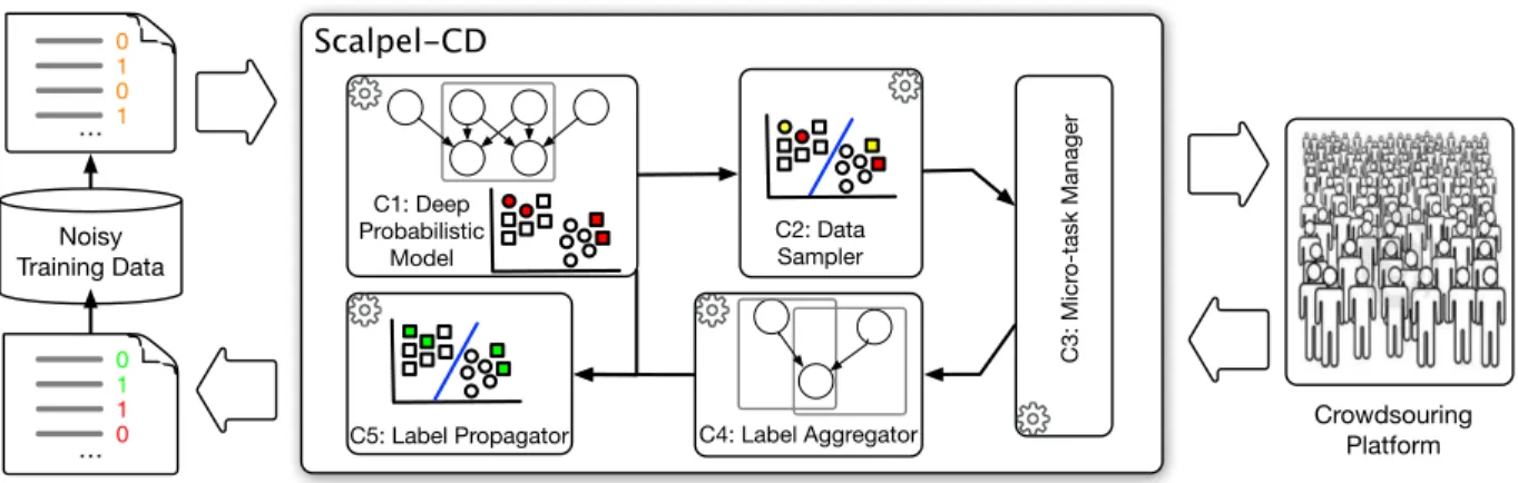
Figure 1 presents a simplified architecture of Scalpel-CD. It takes as input a noisy dataset, e.g., a corpus of documents each associated with a noisy label that represents the polarity (sentiment) of the text. The dataset is first passed to a deep probabilistic model, which infers the latent class for each data instance and a high-level latent feature representation of it. Both outputs are used as input for the data sampler, which calculates the reliability of the model’s inference and the representativeness of the data instance. The data sampler then selects representative data instances whose labels need to be inspected the most. The selected data instances, together with the noisy labels, are passed to the micro-task manager, which dynamically creates human computation tasks and publishes them on a crowdsourcing platform.
The noisy label for each selected data instance is then examined by multiple human workers. Once workers complete their inspec-tion, the results are passed to a label aggregator. The label aggregator aggregates multiple workers’ annotations to obtain the true class for each inspected data instance. The data instances, together with their verified/fixed labels are then fed into a label propagator, which propagates the labels to similar data instances identified through their latent features (inferred by the deep probabilistic model). The data sampler and label aggregator can be seen as down-sampling and up-sampling methods to reduce crowd annotation efforts and amplify crowd contributions, respectively. Together, they help to scale out human contributions, which is of critical importance in a human-in-the-loop approach where human workers are often the bottleneck in terms of scalability or computational efficiency.
2.2
Components
C1: Deep Probabilistic Model. The deep probabilistic model re-ceives a noisy dataset and simultaneously infers two types of latent variables, i.e., the latent class and the latent features. The latent class represents what the model believes is the true label for the data instance. The latent features, represented as low-dimensional vectors, essentially capture the underlying data structure. They are useful in identifying representative data instances for data sam-pling and in identifying similar data instances for label propagation. The inference relies on both the existing noisy label and the latent features. The basic idea is that data instances distributed close to each other in the latent feature space are likely to belong to the same class. Consider for example a data instance whose surround-ing neighbors are all positively labeled; it is likely to be positive also, even when its existing noisy label is actually negative. In most cases, the surrounding neighbors are partially labeled as positive and partially as negative. The deep probabilistic model is able to
Scalpel-CD C2: Data Sampler C3: Micr o-task Manager Crowdsouring Platform Noisy Training Data C4: Label Aggregator C5: Label Propagator C1: Deep Probabilistic Model 0 1 1 0 0 1 0 1 … …
Figure 1: The architecture of Scalpel-CD: our system takes as input a noisy training dataset and identifies data instances with potentially wrong labels; it samples from the data representative instances and involves crowd workers to verify and fix wrong labels; the fixed labels are then propagated to similar data instances in order to scale out the contributions of the crowd. strike a balance between the latent features and the noisy label to
obtain a reasonable estimate of the latent class. This component is described in detail in Section 3.1 and 3.2.
C2: Data Sampler. The data sampler is critical in reducing the annotation effort of the crowd workers as it helps to select repre-sentative data instances for which the deep probabilistic model’s inference is unreliable. The model reliability is approximated by the (inverse) uncertainty of the inference model. The representa-tiveness of a data instance is estimated based on the underlying data structure. Specifically, the data sampler makes use of the latent features inferred by the deep probabilistic model to cluster the data instances. Within each cluster, data instances are supposed to be similar to each other. The data sampler then uses an algorithm to weight the importance of model reliability and data representative-ness when selecting data. More details on the sampling algorithm are presented in Section 3.3.
C3: Micro-Task Manager. The micro-task manager is responsi-ble for dynamically creating human computation tasks that are then published on a crowdsourcing platform. It takes as input data instances (together with their original noisy labels) selected by the data sampler, and builds a Web page to be published on the crowdsourcing platform using a templating engine. Once published, the micro-tasks can be selected by workers on the crowdsourcing platform, who are then asked to verify the noisy labels and fix them if deemed incorrect. The results are sent back to the micro-task manager, which in turns inserts them into the label aggregator. C4: Label Aggregator. Label aggregation is a central problem in crowdsourcing. Given multiple human workers contributing to individual data instances, the label aggregator is designed to infer the true label through a probabilistic latent variable model. A large body of work can be found on this topic, e.g., the classic Dawid-Skene model [8] or the GLAD model [42] (see Section 5). Our work focuses more on addressing the scalability issue of the crowd rather than on quality issues. However, our system supports arbitrary label aggregation methods through a generic interface.
C5: Label Propagator. The label propagator transfers manually examined labels to similar data instances. This is achieved by ex-ploiting the underlying data structure: the noisy labels of data
instances identified by the deep probabilistic model are matched to the verified labels of the data instances in a cluster. For data instances with different verified labels in the same cluster, label matching is performed using a nearest neighbor search. Coupled with the data sampler, the label propagator serves as an amplifier for maximizing the utility of the crowd. The label propagator is de-signed to optimize two criteria: it propagates labels to as many data instances as possible while ensuring that the labels are propagated to the right instances. A detailed introduction to the propagation algorithm is given in Section 3.4.
3
DEEP PROBABILISTIC MODELING AND
CROWDSOURCING TRADEOFFS
Scalpel-CDorchestrates human and machine intelligence via a set of components described in the previous section. These components intrinsically seek a tradeoff between different key factors of our system. In this section, we characterize the tradeoff space into three parts, relevant to the deep probabilistic model, the data sampler, and the label propagator, respectively; for each part, we introduce an algorithmic solution that simplifies the search for the optimal tradeoff as the search for a single system parameter. Note that the label aggregator is also concerned with a tradeoff: the number of crowd contributors involved and the accuracy of result aggregation. However, this has been extensively studied (see [2, 23]). In the following, we first briefly describe our deep probabilistic model, then introduce the algorithmic solutions to the three components.
3.1
Deep Probabilistic Model
To infer the latent class of a data instance, the basic intuition of our deep probabilistic model is that data instances similar to each other are more likely to belong to the same class. We consider a generative model to fully capture the data distribution of a large training dataset. Given a noisy dataset D= {(xi, ˆyi)}i=1N , where xi
is a data instance and ˆy is its corresponding noisy label (we will omit the index i whenever it is clear that we are referring to a single data instance), the deep probabilistic model encompasses the generative modeling of both data and labels, described as follows.
z θ x y γ ˆ y N
Figure 2: Graphical model of our deep probabilistic model. The data instance x and the noisy label ˆy are both generated from distributions conditioned on the latent feature vector zand the latent class y. θ and γ are the parameters of the likelihood function for generating the data and noisy labels, respectively (priors of z and y are omitted).
– Draw a latent feature vector zi ∼ P (z) where P (z) = N (0, I) is a standard Gaussian distribution;
– Draw a latent class yi ∼ P (y) where P (y)= Cat(y|π) is a Multinoulli distribution, whereπ = {1/K, . . . , 1/K}⊺(K is the number of classes);
– Draw a data instance xi ∼ Pθ(x|z, y); – Draw a noisy label ˆy ∼ Pγ(y|z, y).ˆ
Our overall model is depicted in Figure 2. The data instance and the noisy label are both dependent on the latent feature vector z and the latent class y, which captures the class specification. z can contain both class and non-class related features. For example, for a sentence x, the latent feature vector z can represent topics related to a certain class, and additionally, it can capture the author’s writing style that are not class-related. The non-class related features, when mistaken as class-related, are likely to lead to wrong labels during the labeling process. z and y are conditionally dependent given the observed data instance x and the noisy label ˆy.
Formally, the deep probabilistic model is expressed by the fol-lowing factorization:
P (x, ˆy, z, y|θ , γ )= Pθ(x|z, y)Pγ(y|z, y)P (z)P (y).ˆ (1) The likelihood functions Pθ(x|z, y) and Pγ(y|z, y) are parameterizedˆ by deep neural networks to accurately capture the distributions of the data and the noisy labels. Depending on the specific form of the data, different likelihood functions are to be used for Pθ(x|z, y): Gaussian likelihood is suitable for image data, while Multinomial likelihood is more suitable for textual data (see [18, 29]). Pγ(y|z, y)ˆ is represented by a Multinoulli likelihood.
Inference and Learning. The inference for the latent feature vec-tor z and the latent class y is closely related to the learning of the deep probabilistic model parameters. The parameters are learned by maximizing the log likelihood of the observed data instances and the associated noisy labels:
log P (x, ˆy|θ , γ )= log ∬
P (x, ˆy, z, y|θ , γ ) dzdy. (2) Due to the intractability of the integral, we approximate the true pos-teriors of z and y with variational ones, denoted by Qϕ(z|x, y) and Qψ(y|x), respectively. We use a Gaussian distribution for Qϕ(z|x, y)
and a Multinoulli distribution for Qψ(y|x). Given the complex de-pendencies among the low-level features of data instances and their relationships with the latent variables, these distributions are again parameterized by deep neural networks. The parameters, including those of the generation networks θ and γ and those of the inference networks ψ and ϕ, are then learned by maximizing the evidence lower bound (ELBO) [4] of the objective as follows:
EQϕ,ψ(z,y |x)[log Pθ,γ(x, ˆy|z, y)] − DK L[Qϕ,ψ(z, y|x)∥P (z, y)], (3)
where E(·) is expectation and DK L[·∥·] is the KL-divergence be-tween two distributions.
3.2
Inferring the Latent Class
From a neural network perspective, the first part of the ELBO (Equa-tion 3) can be interpreted as the sum of the (negative) reconstruc(Equa-tion errors of the observed feature x and noisy label ˆy, while the second part is the (negative) regularization term preventing overfitting. Hence, we rely both on the data distribution and the existing noisy labels when inferring latent classes.
The original ELBO weights both types of reconstruction errors as equally important. While this can result in a powerful generative model for data and label generation, our goal is different: we are interested in inferring the latent classes, for which the data dis-tribution and the existing noisy labels are likely to be differently important. Furthermore, their importance can vary across different datasets: for datasets whose data distributions are highly indicative of the true class and the noise ratio of the existing labels is high, the data distribution should be more trusted in the inference; otherwise, the existing label should be more trusted.
It is, therefore, natural to extend the ELBO by introducing a parameter β to weight the importance of the two types of recon-struction errors:
EQϕ,ψ(z,y |x)[log Pθ,γ(x, ˆy|z, y)]=
EQϕ,ψ(z,y |x)[log Pγ(y|z, y)]ˆ + β · EQϕ,ψ(z,y |x)[log Pθ(x|z, y)].
(4) In case β , 1, we are no longer optimizing the ELBO on the log marginal likelihood (Equation 2). If β < 1, we would trust more the existing labels than the data distribution; consequently, the model is less able to determine label noise by resorting to the data distribution. Otherwise, if β > 1, we are weakening our trust on the existing noisy labels while putting more trust on the data dis-tribution in determining label noise. While this allows for more flexibility, it could also bring additional noise to the labels due to the non-class related features in the data distribution. Finding a proper value of β is important to achieve a good performance in inferring latent classes.
The resulting optimization algorithm is given in Algorithm 1. It iteratively goes over two steps, i.e., the forward and the backward step. In each iteration, the forward step (row 5) computes the latent variables given the current parameters; the backward step (row 6-8) then updates the parameters by backpropagating the gradients of the errors. In the calculation of the gradients (row 6), we use an adapted version of the ELBO (Equation 4).
3.3
Data Sampling
The data sampler selects representative data instances for which our deep probabilistic model’s inference is most unreliable. The
Algorithm 1: Learning the Deep Probabilistic Model Input: the set ofN i.i.d. data instances D = {xi, ˆyi}Ni=1, ELBO
adapterβ, and the maximum number of iterations I ter
1 Initializeϕ, ψ, θ, γ ; 2 fort = 1; t ≤ Iter ; t + + do
3 Sample a batch of data instances;
4 forall xi ∈ the batch do 5 Computeyiand zi;
6 Compute the noisy gradient∆ϕ,ψ , θ ,γL ; 7 Average noisy gradients from batch;
8 Updateϕ, ψ, θ, γ with gradient descent; 9 if ELBO has converged then
10 break;
model reliability is approximated by the inverse of the model’s uncertainty, measured by Shannon entropy [13, 37]:
H [y|x]= −
K
Õ
C=1
p(y= C|x) logp(y = C|x) (5) where C is the class and K is the number of classes. We hypothesize that uncertainty sampling is effective for datasets with random noise: for data instances far away from the true decision boundary, the deep probabilistic model can take advantage of the majority label of data instances and provide correct inference; however for data instances close to the decision boundary, the deep probabilistic model will have a high uncertainty due to the mix of data instances from different classes and will likely result in some wrong inference. However, for a dataset with structural noise, since there can exist certain regions of the data distribution where the majority of the labels are incorrect, the inference of the deep probabilistic model can be totally off while being highly probable according to the model. Therefore, we also consider random sampling, which is independent of the deep probabilistic model. The effectiveness of the two sampling methods can be evaluated using a set of validation instances with ground truth labels: a better sampling method is the one from which the sampled data instances covers more validation instances where the deep probabilistic model’s inference is wrong. An additional criterion for data sampling is the representative-ness of the data instances, which is important for label propagation. We apply a clustering method to the data instances in the latent feature space as uncovered by the deep probabilistic model, i.e., zi (1 ≤ i ≤ N ). Data instances falling into the same clusters are supposed to be more similar with each other.
We now describe our data sampling algorithm (see Algorithm 2). It starts by clustering data instances based on their latent features (row 1), then chooses a sampling strategy between uncertainty and random sampling based on the coverage of validation instances for which model inference is wrong (row 3). Then, given a budget B, i.e., the predefined number of data instances to be inspected by the crowd, the data sampler first ranks the data instances in each cluster according to the sampling strategy (row 5). It then selects from each cluster the top-ranking data instances (row 7). The number of data instances selected in each cluster is proportional to the size of the cluster (row 6). Note that for random sampling, selecting data from clusters proportionally is equivalent to stratified random sampling.
Algorithm 2: Data Sampling
Input: Data instances represented by latent features and inferred classes D= {zi, P (yi)}Ni=1, budgetB, #clusters c, validation
instances with ground truth labels V
Output: Data instances sampled S ⊂ D, clusters C= {Cj}cj=1 1 C ← Cluster data instances D based on latent features; 2 S ← ∅;
3 Decide the sampling strategy using V;
4 foreach Cj ∈ Cdo
5 Rank data instances in Cjaccording to the sampling strategy; 6 nj← j|C j| N ×B k ;
7 Sj← Picknjtop-ranking data instances; 8 S ← S ∪ Sj;
A key parameter of the algorithm is the number of clusters, de-noted by c ≤ B. By setting this parameter to different values, the data sampler weights the importance of data representativeness and model reliability differently. Consider the extreme case when c = 1, i.e., no data partitioning, the data sampler fully relies on uncertainty or random sampling for selecting data instances; when c= B, i.e., a single data instance is selected from each cluster, the data sampler relies more on data representativeness for selecting data instances. Our algorithm is not restricted to any specific clus-tering methods. The only requirement is the flexibility for users to specify the number of clusters c. As an example, we consider the widely used K-means method for clustering. Comparison of different clustering methods is left for future work.
3.4
Label Propagation
The label propagator amplifies the crowd contributions by prop-agating corrected labels to similar data instances. The similarity between data instances is calculated as the Euclidean distance be-tween the latent feature vectors of the instances. A key parameter of the label propagating algorithm is the number of data instances to propagate the label to. Given that the size of the clusters are dif-ferent and that data instances within each cluster are similar, we use a relative number for the parameter to represent the fraction of the data instances for label propagation in each cluster. We denote this parameter as p. A small value of p will affect fewer data instances, thus being less efficient in scaling out human contributions; on the contrary, a big value of p, while being efficient, might increase the noise ratio of the dataset as labels can get wrongly propagated. A proper setting of p is, therefore, of key importance for scaling out human contributions in a reliable way.
Our label propagation algorithm is presented in Algorithm 3. It performs label propagation in each cluster identified by the data sampler. For each inspected data instance in the cluster (row 1-2), the label propagator first ranks the data instances that have not been inspected by crowd workers according to their distance to the inspected instances (row 3-5). It then picks the top ranking instances with shortest distances (row 6). Finally, for each of the selected data instances in the cluster, the label of the nearest inspected data instance is propagated (row 7-8).
Algorithm 3: Label Propagation
Input: Data instances represented by latent features D= {zi, ˆyi}i=1N ,
data instances with fixed labels S= {zh, yh}h=1H , clusters
C= {Cj}cj=1, propagation fractionp
Output: Fixed labels D= {yi}i=1N 1 foreach Cj ∈ Cdo
2 foreachh ∈ S ∧ h ∈ Cjdo 3 foreachi ∈ Cj∧i < S do
4 di, h ← distance between zhand zi; 5 Rank data instancei (i ∈ Cj∧i < S) by di, h;
6 Ph←p × | Cj| top ranking instances with smallestdi, h; 7 foreachi ∈ Ðh=1H Phdo
8 yi←yh∗whereh∗= arg min di, h(i ∈ Ph);
4
EXPERIMENTS AND RESULTS
This section presents experimental results for evaluating the per-formance of Scalpel-CD. We start by presenting an evaluation of each of its components by answering the following questions: •Q1: How well does the deep probabilistic model perform when
inferring the latent class from noisy data?
•Q2: How well do the uncertainty and random sampling perform on datasets of different noise types?
•Q3: How effective is label propagation (together with data sam-pling) in scaling out the contributions of crowd workers? From a human computation perspective, while we mainly consider improving the scalability of the crowdsourcing process, we also in-vestigate the quality of the work performed by the crowd, which we report when addressing Q3. Subsequently, we evaluate the system as a whole by considering the following issue:
•Q4: Does our proposed Scalpel-CD system outperform the state-of-the-art methods for debugging noisy labels?
In addition, we also investigate how much Scalpel-CD helps in improving the performance of a machine learning system. In the following, we start by introducing our experimental setup, before answering each of the above questions in a separate subsection.
4.1
Experimental Setup
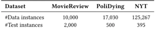
Datasets. We experiment with three datasets created with differ-ent noise types, namely MovieReview (random noise), PoliDying (structural noise), and NYT (structural noise). These datasets are representative for sentiment analysis, event detection, and relation extraction, respectively. The MovieReview dataset [30] is a subjec-tivity classification dataset of movie reviews from Rotten Tomatoes. This dataset contains ground truth labels for all data instances; we, therefore, simulate wrong labels by randomly selecting a cer-tain fraction (10% to 50%) of the data instances and flipping the ground truth labels. The PoliDying dataset is a tweet relevance clas-sification dataset for detecting politician-dying events. Following previous studies [20, 36], the positive tweets were retrieved with detailed information on 11 seed events, including event name and date, while negative tweets were retrieved with “politician”- and “death”-related keywords. A set of 500 tweets were manually anno-tated for evaluation. The NYT dataset [33] is a relation extraction dataset for extracting relations from New York Times articles. We
Table 1: Statistics of the datasets in our experiments. Dataset MovieReview PoliDying NYT #Data instances 10,000 17,030 125,267 #Test instances 2,000 500 395
focus on the relation “location-contains”. The dataset is labeled by distant supervision using Freebase as the labeling source. In this dataset, there are 395 manually annotated data instances.
For each of the three datasets, the data sampler selects a num-ber (i.e., the budget B) of data instances for crowdsourcing. We experiment with the budget varying in {50, 100, 200, 500, 1000}. Key statistics from these datasets are presented in Table 1.
Comparison Methods. Due to the lack of existing human-in-the-loop approaches in debugging training data, we compare the fol-lowing automatic methods and our proposed system. 1) Ratio [5]: a ratio-based method that finds the most predictive features and identifies data instances with the most uncertain labels as those containing such features yet labeled differently from the label indi-cated by the features. The predictive power of a feature is calculated as the ratio between the number of data instances of a certain class containing such a feature and the overall number of data instances. 2) Pattern [39]: a generative model designed to capture the label-ing process as a generative process from the latent classes. The model facilitates the inference of the posterior of the latent class given the observed features. However, unlike our deep probabilistic model that infers the latent class by exploiting the data distribu-tion in the latent feature space, Pattern is a probabilistic model that directly models the generative process of low-level features. 3) HierTopic [1]: a hierarchical topic model that assumes a latent topic-word hierarchy for the data generation process. Unlike our probabilistic model which learns complex hidden data structures, HierTopic is only capable of learning a hierarchical structure. For our proposed system, we compare an automated variant and the full system involving human workers: 4) DPM, our proposed deep probabilistic model, which is used in isolation to automatically cor-rect wrong labels. 5) Scalpel-CD, our proposed human-in-the-loop system which makes use of both the deep probabilistic model and crowd workers.
To demonstrate the effectiveness of our system on machine learn-ing tasks, we compare the followlearn-ing trainlearn-ing data configurations: 1) the original noisy training data; 2) training data denoised by the deep probabilistic model; and 3) training data denoised by Scalpel-CD. We apply and evaluate state-of-the-art machine learn-ing models on these different data configurations: we use Convolu-tional Neural Network [16] for MovieReview and PoliDying and Piecewise Convolutional Neural Network (PCNN) [48] for NYT. Parameter Settings and Model Training. We empirically set optimal parameters based on a held-out validation set that contains 10% of the test data. These include the hyperparameters of the deep probabilistic model and the parameters of the trade-off algorithms, i.e., β, c, and p. For the deep probabilistic model, we use a shared embedding layer as the first layer of the inference networks, i.e., Qϕand Qψ, to encode the textual features. We apply a grid search in {32, 64, 128, 256, 512} for the dimension of the embeddings and that of the hidden layers, and we explore multi-layer perceptron
networks with 0, 1, and 2 hidden layers for both the generation and inference models, subject to the constraint that Pθ and Qϕ
have a symmetric architecture (similar to an auto-encoder). We use Adam [17] for model training with mini-batches of 128 data samples for all datasets. The deep probabilistic model is trained for 200 epochs on each dataset and the one with the best performance on the validation set is kept for evaluation.
Evaluation Protocols. We separately evaluate the performance of Scalpel-CD on debugging noisy labels and its effect on the final machine learning tasks using different protocols. For the former task, we take the entire dataset as input. This includes the data instances in the test set together with their noisy labels. The system debugs labels in the whole dataset. The denoised labels of data instances in the test set are then compared against the ground truth. For the final machine learning tasks, our system debugs labels in the training set only. A state-of-the-art deep learning model is then trained on the denoised training set and evaluated on the test set. Two metrics are used to measure the performance of our proposed system in debugging noisy labels and its effect on the final machine learning tasks: accuracy and Area Under the ROC Curve (AUC). Higher accuracy and AUC values indicate better performance.
4.2
Inferring the Latent Class (Q1)
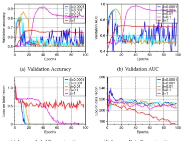
To understand the effectiveness of our deep probabilistic model in inferring the latent class, we analyze the relationship between capturing the data distribution and inferring the latent class. The analysis is carried out by comparing the performance of the deep probabilistic model with different settings of β, which controls the importance of the reconstruction errors of data instances and the noisy labels in the objective function. We analyze the dynamics of our deep probabilistic model on the validation set during the training process, with β selected from {0.0001, 0.001, 0.01, 0.1, 1}. Results on the MovieReview dataset with a noise ratio N R= 20% are shown in Figure 3. We discuss below the influence of different datasets and noise ratios on the performance of the model.
From Figures 3(a-b), we observe a general pattern across dif-ferent settings of β: when the training proceeds, the performance of the deep probabilistic model first increases then decreases. The difference between the performance across β settings indicates that the optimal performance is hit at different performance levels and epochs during the training process: from β = 0.0001 to 0.1, the optimal performance grows and is reached later in the training process for larger values of β; then from β= 0.1 to 1, the optimal performance decreases and is reached earlier. Given such results, we speculate that β= 0.1 best infers the latent classes as it strikes a bal-ance between minimizing the reconstruction errors of the data and the noisy labels. In addition, we further hypothesize that there is a consistent relationship between the level of optimal performance and the time at which it is reached in the training process.
These hypotheses are confirmed by Figures 3(c-d). For small val-ues of β (0.0001−0.01), the deep probabilistic model quickly reaches the minimum reconstruction error of noisy labels. As a result, the in-ferred latent classes are biased towards existing noisy labels, which is evidenced by the optimal accuracy of β = {0.0001, 0.001} be-ing only slightly higher than 0.8 (Figure 3(a); the performance of β = 0.01 is slightly higher yet still not optimal). For β = 1, the
β=0.0001 β=0.001 β=0.01 β=0.1 β=1 V a lid a tio n a ccu ra cy 0.5 0.6 0.7 0.8 0.9 Epochs 0 20 40 60 80 100
(a) Validation Accuracy
β=0.0001 β=0.001 β=0.01 β=0.1 β=1 V a lid a ti o n AU C 0.4 0.6 0.8 1.0 Epochs 0 20 40 60 80 100 (b) Validation AUC β=0.0001 β=0.001 β=0.01 β=0.1 β=1 L o ss o n l a b e l re co n . 0 0.5 1.0 Epochs 0 20 40 60 80 100
(c) Loss on Label Reconstruction
β=0.0001 β=0.001 β=0.01 β=0.1 β=1 L o g o n d a ta re co n . 180 200 220 240 260 Epochs 0 20 40 60 80 100
(d) Loss on Data Reconstruction
Figure 3: Comparison of performance against loss in data and label reconstruction with different settings of β on the MovieReview dataset. Upper figures are the dynamics of ac-curacy (a) and AUC (b) on the validation set during the train-ing process; lower figures are the reconstruction loss (nega-tive log-likelihood) of noisy labels (c) and data instances (d). reconstruction error of the data is significantly reduced (more than for other settings, see Figure 3(d)); the reconstruction error of noisy labels is however not reduced as much as in the other settings (Fig-ure 3(c)). The inferred latent classes therefore cannot benefit from those existing correct labels. To infer the latent class in an unbiased manner, sufficient model training has to be performed to reduce both types of reconstruction errors. This implies that the optimal setting of β is most likely the one that takes most of the time to reach the optimal performance during the training process. Impact of Datasets and Noise Ratios. We observe similar results with the other datasets. The optimal settings of β are 1 and 0.01 for PoliDying and NYT, respectively. The variation across datasets implies different utility of the data distribution in inferring the latent class, which highlights the importance of searching for the optimal β separately for different datasets. Actual performance using these β values will be reported in Section 4.5. We note that our model is robust with respect to different noise ratios. It achieves accuracy scores > 0.9 even when the noise ratio of MovieReview goes up to 40%. Compared with noise ratios, model performance is more affected by the predictive power of the data distribution. We remark, however, that the model can always benefit from the data distribution and achieve better performance than 1 − N R.
4.3
Uncertainty and Random Sampling (Q2)
The data sampling component of Scalpel-CD allows for two sam-pling strategies, i.e., uncertainty samsam-pling and random samsam-pling, which are model-dependent and model-independent, respectively. We therefore hypothesize that random sampling is more effective than uncertainty sampling for datasets with structural noise. To verify our hypothesis, we conduct a comparative analysis between the MovieReviews dataset and the PoliDying and NYT datasets,
Positive Negative −40 −20 0 20 40 −60 −40 −20 0 20 40 60
(a) Noisy Label in Latent Space
Positive Negative −40 −20 0 20 40 −60 −40 −20 0 20 40 60
(b) Inferred Class in Latent Space
Data w/ correct inference Data w/ wrong inferrence
−40 −20 0 20 40 −60 −40 −20 0 20 40 60
(c) Correct and Wrong Inference
Not selected by uncertanty Selected by uncertainty −40 −20 0 20 40 −60 −40 −20 0 20 40 60 (d) Uncertainty Sampling All - random Wrong - random All - uncertainty Wrong - uncertainty C o ve ra g e 0.2 0.4 0.6 0.8 1.0
Perc. of Selected Instances 0.1 0.2 0.3 0.4 0.5
(e) Coverage - MovieReview
Positive Negative −50 0 50 −100 −50 0 50 100
(f) Noisy Label in Latent Space
Data w/ correct inference Data w/ wrong inference −50
0 50
−100 −50 0 50 100
(g) Correct and Wrong Inference
Not selected by uncertainty Selected by uncertainty −50 0 50 −100 −50 0 50 100 (h) Uncertainty Sampling
Not selected by random Selected by random −50
0 50
−100 −50 0 50 100
(i) Random Sampling
All - random Wrong - random All - uncertainty Wrong - uncertainty C o ve rg a e 0 0.1 0.2 0.3 0.4 0.5
Perc. of Selected Instances 0.1 0.2 0.3 0.4 0.5
(j) Coverage - PoliDying
Figure 4: Effects of uncertainty and random sampling on the MovieReview dataset (upper figures) and the PoliDying dataset (lower figures). From left to right, upper figures are the visualization of the noisy label (a) and the inferred latent class (b) in the two dimensional latent feature space; visualization of the data instances with correct and wrong inference of the latent class (c) and those selected (top-10%) and not selected by uncertainty sampling (d). Lower figures are the visualization of the noisy labels (f) and the data instances with correct and incorrect inference of the latent class (g) in the latent feature space; visualization of the (top-)10% selected and not selected data instances by uncertainty sampling (h) and random sampling (i). Figures on the right part are the coverage of the uncertainty sampling and random sampling on the entire validation set and the subset where the inference is wrong for the MovieReview dataset (e) and the PoliDying dataset (j).
as the two types of noisy datasets. The comparison is carried out by 1) visually locating in the latent feature space the selected data instances using the two sampling strategies and the data instances where the inference of the latent classes is wrong, and 2) statis-tically comparing the coverage of the selected data instances on data instances where the inference is wrong. (For rigorousness, we use the validation set for comparison, however similar results are observed in the test set.)
We start by investigating the effectiveness of uncertainty sam-pling on the MovieReview dataset. We apply t-SNE [26] to embed the latent features of the data instances into a two-dimensional space, and then visualize the noisy label and the inferred latent class in Figures 4(a-b). Given our previous results (high performance of our deep probabilistic model in latent class inference in Figures 3(a-b)), we observe from Figures 4(a-b) that the inferred latent features are highly indicative of the latent class: data instances of different classes are located separately in the latent feature space. Figure 4(c) then shows the data instances for which the inference is correct and wrong in two colors, respectively. We observe that our model can effectively recover the true classes of data instances located far away from the model’s decision boundary. In contrast, the majority of the data instances with wrong class inference are located close to the decision boundary. This is due to the fact that at the decision boundary, data instances of different classes are mixed with each other, leading to high model uncertainty. This is confirmed by Fig-ure 4(d), which visualizes the top-10% data instances selected by uncertainty sampling. Comparing Figures 4(c) and 4(d), we observe that uncertainty sampling is a highly effective method in selecting data instances when the model inference is wrong.
For comparison, we show the effect of uncertainty sampling and random sampling on the PoliDying dataset created with structural
noise. Figure 4(f) visualizes the noisy labels in the latent feature space and 4(g) shows the data instances with correct and wrong inference in two colors. We can observe that the deep probabilistic model can be totally wrong in its inference for a set of data instances close with each other (i.e., those about the same topic), e.g., the red clusters in Figure 4(g). Comparing such a result to Figure 4(f), we observe that the noisy labels for these data instances are almost all incorrect. These highly consensual yet wrong labels not only make the inference wrong, but also lead to high model confidence (i.e., low uncertainty). This is validated by Figure 4(h), which shows that uncertainty sampling can hardly identify data instances with structural errors. In contrast, Figure 4(i) shows a similar number of data instances (both 10%) selected by random sampling, which is able to cover data instances with wrong inference scattered at different regions of the latent feature space.
Impact of Noise Types. To quantitatively compare uncertainty and random sampling, Figures 4(e,j) show for both datasets the coverage of the selected data instances (from 10% to 50%) on the entire validation set and the subset where the model inference is wrong. On one hand, we observe that for MovieReview, uncertainty sampling is highly capable of selecting those data instances with wrong inference (80% covered by 20% selected instances). On the other hand, random sampling performs much better for PoliDying. These results highlight the distinct capabilities of uncertainty sam-pling at tackling random noise and of random samsam-pling at tackling structural noise. Finally, we note that for the NYT dataset the two sampling strategies perform comparably well. This is likely due to the variety of the entity pairs (tens of thousands) in the external database used for labeling, which comes in contrast to the PoliDy-ing dataset that uses a limited number of seed events and keywords as labeling sources.
c=1 c=10 c=20 c=50 Accu ra cy 0.78 0.80 0.82 Propagation rate 0 0.2 0.4 0.6 0.8 1.0
(a) Expert - Accuracy
c=1 c=10 c=20 c=50 AU C 0.75 0.80 0.85 Propagation rate 0 0.2 0.4 0.6 0.8 1.0 (b) Expert - AUC c=1 c=10 c=20 c=50 Accu ra cy 0.76 0.78 0.80 0.82 Propagation rate 0 0.2 0.4 0.6 0.8 1.0 (c) Crowd - Accuracy c=1 c=10 c=20 c=50 AU C 0.72 0.74 0.76 0.78 0.80 Propagation rate 0 0.2 0.4 0.6 0.8 1.0 (d) Crowd - AUC
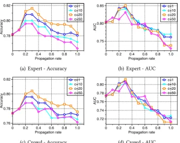
Figure 5: Effect of label propagation with different settings of the propagation rate and the number of clusters on the PolyDying dataset. Upper figures are the results with expert-contributed labels measured by accuracy (a) and AUC (b); lower figures are the results with crowd-contributed labels measured by accuracy (c) and AUC (d).
4.4
Scaling out Human Contributions (Q3)
We now investigate the effectiveness of data sampling and label propagation for scaling out human contributions. The relevant system parameters are the number of clusters c, which controls the importance of the representativeness of data instances in data sampling, and the fraction of data instances p in each cluster to be considered for label propagation. We analyze the impact of different settings of p from 0 to 1 with a step of 0.1, and c selected from {1, 10, 20, 50}. Furthermore, we conduct a comparative study between labels verified by experts and crowd workers to understand the im-pact of imperfect human work. We report results on the PoliDying dataset with a budget B= 500. Similar results are observed on the NYT dataset; results for the MovieReview dataset and the impact of different budgets will be analyzed below.
Figures 5(a-b) show the results of expert verified labels. When p increases from 0 to 1, we observe inverse U-shaped curves across all different settings of c and the two metrics: the performance first increases then decreases, with optimal performance reached at p= 0.3. This indicates that label propagation does help in correct-ing more data instances not inspected by experts. The performance decreases from p = 0.3 to 1 since the propagation accuracy de-creases when labels are propagated to data instances semantically different from the manually verified ones. Comparing the different settings of c, we observe that label propagation reaches its best per-formance at c= 20, which significantly outperforms other settings. This confirms the importance of finding an optimal setting for c to make the best partitioning of the data and the optimal tradeoff between the different criteria for data sampling.
For our crowdsourcing experiment, we solicit from the crowd three labels for each data instance. Results show that crowd labels match expert labels on 84.73% data instances. With such an accuracy,
we do not observe consistent patterns of performance variation in label propagation. A simple filtering of data instances where all three crowd workers agree results in 81.50% remaining data instances, whose labels match expert labels 90.20% of the time. Figures 5(c-d) show the label propagation results on the filtered labels. We observe similar patterns with expert labels (Figures 5 (a-b)). Overall, label propagation enhances system performance by 3.5% (accuracy) and 4.6% (AUC) for expert labels and by 2.1% (accuracy) and 3.8% (AUC) for crowd labels.
Impact of Budgets and Datasets. We observe similar results for budget B= 1000 on both the PoliDying and NYT datasets. However, for B <= 200 no explicit patterns are observed. This is likely due to the under-representativenes of the inspected data instances. For MovieReview, crowd contributions improve the resulting accuracy from 0.925 to 0.956 and the AUC from 0.977 to 0.987. However, the performance gets worse for p >= 0.1. This is mainly due to the effectiveness of the deep probabilistic model in making use of data distributions to correct erroneous labels in a dataset with random noise (see Figures 3(a-b) and Section 4.5), which makes it difficult to further improve label quality through label propagation.
4.5
Performance on Debugging Labels (Q4)
We now compare the performance of our proposed system to state-of-the-art methods for debugging noisy labels. Table 2 (“Debug-ging”) reports their performance on our three datasets. From these results, we make the following observations.
Ratio works well on the MovieReview dataset, however fails on PoliDying and NYT (compared to the original labels). Pattern, as a probabilistic method, is more robust: it improves label quality for both MovieReview and PoliDying. Yet, it still fails on the NYT dataset. Recall that both methods use the low-level features (i.e., words) for label inference. These results indicate that probabilistic methods that capture data distributions based on low-level features do not necessarily work for debugging noisy labels. In contrast, HierTopic, which models a hierarchical structure from the data using a probabilistic framework, consistently improves the label quality across all datasets. These results confirm the importance of considering data structures in debugging noisy labels.
Our proposed deep probabilistic model outperforms all the other methods by a large margin: it yields an average improvement of 7.0% in accuracy and 3.9% in AUC compared to HierTopic; compared with the original noisy labels, it improves the label quality by 9.1% in accuracy and 11.8% in AUC. These results clearly indicate the effectiveness of our model in debugging noisy labels. In particular, the improvements over HierTopic shows that deep neural networks are effective in learning the underlying data structure. Furthermore, the effectiveness of the model on PolyDying and NYT indicates that, overall, the model works well for datasets with structural noise, even if the inference can be unreliable for data instances distributed in certain regions of the latent feature space (Section 4.3).
Scalpel-CDachieves the best performance across all datasets. It outperforms the deep probabilistic model by 3.8% in accuracy and 3.9% in AUC on average. This highlights the value of human input in the process. Compared to the original noisy labels, our system improves label quality by 12.9% in accuracy and 15.8% in AUC, with only 2.8% data instances manually inspected by the crowd.
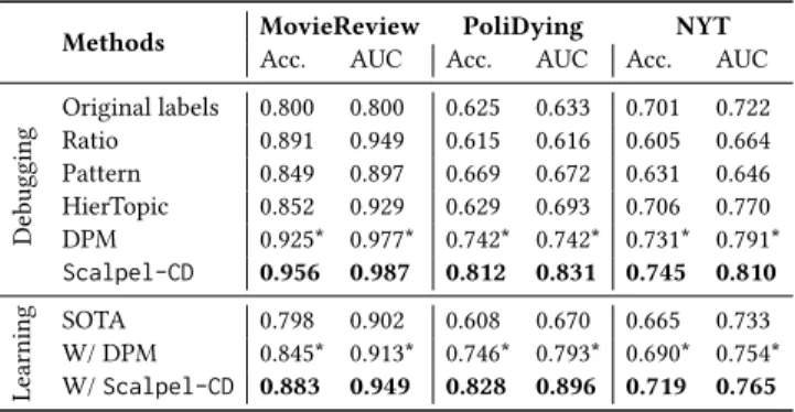
Table 2: Performance of the compared methods on two set-tings: debugging noisy labels and machine learning. Results on the MovieReview dataset are reported for N R= 20%. Re-sults of our proposed systems are obtained with a budget B = 500. The best performance for each dataset in each set-ting is boldfaced; the runner up is labelled with “*”.
Methods MovieReview PoliDying NYT Acc. AUC Acc. AUC Acc. AUC
Debugging Original labels 0.800 0.800 0.625 0.633 0.701 0.722 Ratio 0.891 0.949 0.615 0.616 0.605 0.664 Pattern 0.849 0.897 0.669 0.672 0.631 0.646 HierTopic 0.852 0.929 0.629 0.693 0.706 0.770 DPM 0.925* 0.977* 0.742* 0.742* 0.731* 0.791* Scalpel-CD 0.956 0.987 0.812 0.831 0.745 0.810 Learning SOTA 0.798 0.902 0.608 0.670 0.665 0.733 W/ DPM 0.845* 0.913* 0.746* 0.793* 0.690* 0.754* W/ Scalpel-CD 0.883 0.949 0.828 0.896 0.719 0.765 Impact on Learning Tasks. The benefits of using our system on machine learning tasks is shown in Table 2 (“Learning”). The perfor-mance of state-of-the-art learning methods improves significantly when using our deep probabilistic model or our system as a whole. On average, machine learning performance is improved by 12.0% in accuracy and 10.2% in AUC using Scalpel-CD. These results clearly highlight the benefits of debugging noisy labels and the effectiveness of Scalpel-CD on machine learning tasks.
5
RELATED WORK
This section gives an overview of relevant work from the emerg-ing field of human-in-the-loop paradigm for artificial intelligence (HITL-AI) and from label noise reduction for training data. HITL-AI. Human computation and machine learning are increas-ingly interweaving with each other [41]. The main intersection is crowdsourced training data creation, e.g., the ImageNet dataset for computer vision [10] and many crowd annotated datasets for various natural language processing tasks [14, 28]. A closely re-lated line of work in the machine learning community is “learn-ing from crowds”, where researchers study models that can learn from noisy labels contributed by crowds [32, 40, 46, 47]. Unlike the conventional learning setting, models developed in this con-text are concerned with learning parameters of the annotation process (e.g., annotator expertise [32] and task difficulty [46]) and inferring true labels from noisy ones. Such an idea has been ex-tended to incorporate (deep) active learning to reduce annotation efforts [12, 40, 45, 47].
In contrast to creating high-quality training data from scratch, e.g., through active learning from the crowd, fast creation of training data with noise tolerance is becoming more popular [2, 31]. Existing work on debugging machine learning systems mainly focuses on identifying the weakest component. Much fewer approaches have considered debugging training data, which is a key bottleneck for improving machine learning systems [6]. Existing work is mainly developed within the topic of interpretability and transparency of machine learning models [34]. These work mainly uses perturbation based approaches to identify data instances that are likely to cause incorrect predictions [7, 19, 24]. Unlike these work that requires
incorrect predictions to be observed, our deep probabilistic method is a self-discovering method as the identification of erroneous labels only relies on data distributions; more importantly, our system involves humans for reliable label correction.
Label Noise Reduction. Existing methods have been developed separately for distant supervision and crowdsourcing. Methods in the former context mainly leverage data distributions in the low-level feature space, e.g., the factor graph model by Riedel et al. [35] and the generative model by Takamastu et al. [39]. Alfonseca et al. [1] introduce a hierarchical model to capture the data distribu-tion in the topic space. In comparison, our deep generative model is flexible to capture data distributions with more complex data struc-tures. In crowdsourcing, label noise reduction has been a central problem as worker annotations are often noisy. Typical methods assume a redundancy of worker annotations [22, 38], e.g., majority voting and those based on Expectation Maximization (EM) [8]. EM methods simultaneously estimate the true labels and parameters of the annotation process, e.g., worker reliability by Dawid and Skene [8] and task difficulty by Whitehill et al. [42]. These methods are, however, not applicable to most machine learning scenarios where each data instance is labeled only once. Our work is different in that we consider the broader scope of noisy training data, where labels are not necessarily redundant.
Finally, our work is also related to the broader domain of data cleaning, mainly studied by the database community [21, 43, 44]. Yakout et al. [44] study an approach to automatically generate data cleaning rules for relational databases. Krishnan et al. [21] specifically focus on cleaning training sets for convex statistical models (e.g., SVM, Logistic Regression). They introduce an SGD-like method that leverages expected model improvement to identify the most beneficial data instances to be cleaned. The method, how-ever, does not apply to deep learning models. Most importantly, all existing work does not explicitly consider the human’s role in data cleaning and does not address the potential issues of human involvement (e.g., scalability and work quality).
6
CONCLUSION
We presented Scalpel-CD, a new human-in-the-loop system that exploits the complementary strength of humans and machines for debugging noisy training data. Scalpel-CD leverages deep proba-bilistic modeling to identify data instances with potentially wrong labels and infer their latent classes, and engages humans to inspect specific data instances for which the model inference is of low reli-ability. Scalpel-CD is a generic system applicable to any type of training data and can be easily optimized for specific datasets. Our extensive evaluation on multiple machine learning datasets with different noise types demonstrates that Scalpel-CD significantly improves label quality and machine learning performance with minimum human involvement. As future work, we plan to study how to best involve humans to increase the explainability of the models and to reduce potential biases in automated decisions.
ACKNOWLEDGEMENT
This project has received funding from the European Research Council (ERC) under the European Union’s Horizon 2020 research and innovation programme (grant agreement 683253/GraphInt).
REFERENCES
[1] Enrique Alfonseca, Katja Filippova, Jean-Yves Delort, and Guillermo Garrido. 2012. Pattern learning for relation extraction with a hierarchical topic model. In Proceedings of the 50th Annual Meeting of the Association for Computational Linguistics (ACL). Association of Computational Linguistics, 54–59.
[2] Alexander Ratner Stephen H Bach, Henry Ehrenberg, Jason Fries, Sen Wu, and Christopher Ré. 2017. Snorkel: Rapid training data creation with weak supervision. Proceedings of the VLDB Endowment (PVLDB) 11, 3 (2017).
[3] Michael S Bernstein, Greg Little, Robert C Miller, Björn Hartmann, Mark S Ackerman, David R Karger, David Crowell, and Katrina Panovich. 2015. Soylent: a word processor with a crowd inside. Commun. ACM 58, 8 (2015), 85–94. [4] David M Blei, Alp Kucukelbir, and Jon D McAuliffe. 2017. Variational inference:
A review for statisticians. J. Amer. Statist. Assoc. 112, 518 (2017), 859–877. [5] Andrew Carlson, Justin Betteridge, Richard C Wang, Estevam R Hruschka Jr,
and Tom M Mitchell. 2010. Coupled semi-supervised learning for information extraction. In Proceedings of the 3rd ACM International Conference on Web Search and Data Mining (WSDM). ACM, 101–110.
[6] Aleksandar Chakarov, Aditya Nori, Sriram Rajamani, Shayak Sen, and Deepak Vijaykeerthy. 2016. Debugging machine learning tasks. arXiv preprint arXiv:1603.07292 (2016).
[7] Anupam Datta, Shayak Sen, and Yair Zick. 2016. Algorithmic transparency via quantitative input influence: Theory and experiments with learning systems. In Security and Privacy (SP), 2016 IEEE Symposium on. IEEE, 598–617.
[8] Alexander Philip Dawid and Allan M Skene. 1979. Maximum likelihood estima-tion of observer error-rates using the EM algorithm. Applied Statistics (1979), 20–28.
[9] Mostafa Dehghani, Hamed Zamani, Aliaksei Severyn, Jaap Kamps, and W Bruce Croft. 2017. Neural ranking models with weak supervision. In Proceedings of the 40th International ACM SIGIR Conference on Research and Development in Information Retrieval (SIGIR). ACM, 65–74.
[10] Jia Deng, Wei Dong, Richard Socher, Li-Jia Li, Kai Li, and Li Fei-Fei. 2009. Ima-genet: A large-scale hierarchical image database. In Proceedings of the 2009 IEEE Conference on Computer Vision and Pattern Recognition (CVPR). IEEE, 248–255. [11] Finale Doshi-Velez and Been Kim. 2017. Towards a rigorous science of
inter-pretable machine learning. arXiv preprint arXiv:1702.08608 (2017).
[12] Meng Fang, Xingquan Zhu, Bin Li, Wei Ding, and Xindong Wu. 2012. Self-taught active learning from crowds. In Proceedings of the 12th IEEE International Conference on Data Mining (ICDM). IEEE, 858–863.
[13] Yarin Gal, Riashat Islam, and Zoubin Ghahramani. 2017. Deep bayesian active learning with image data. Proceedings of the 34th International Conference on Machine Learning (ICML), 1183–1192.
[14] Michael Heilman and Noah A Smith. 2010. Rating Computer-generated questions with Mechanical Turk. In Proceedings of the NAACL HLT 2010 Workshop on Creating Speech and Language Data with Amazon’s Mechanical Turk. 35–40. [15] Armand Joulin, Laurens van der Maaten, Allan Jabri, and Nicolas Vasilache.
2016. Learning visual features from large weakly supervised data. In European Conference on Computer Vision (ECCV). Springer, 67–84.
[16] Yoon Kim. 2014. Convolutional neural networks for sentence classification. arXiv preprint arXiv:1408.5882 (2014).
[17] Diederik P Kingma and Jimmy Ba. 2014. Adam: A method for stochastic opti-mization. arXiv preprint arXiv:1412.6980 (2014).
[18] Diederik P Kingma and Max Welling. 2013. Auto-encoding variational bayes. In Proceedings of the 2nd International Conference on Learning Representations (ICLR).
[19] Pang Wei Koh and Percy Liang. 2017. Understanding black-box predictions via influence functions. In International Conference on Machine Learning (ICML). 1885–1894.
[20] Alexander Konovalov, Benjamin Strauss, Alan Ritter, and Brendan O’Connor. 2017. Learning to extract events from knowledge base revisions. In Proceedings of the 26th International Conference on World Wide Web (WWW). IW3C2, 1007–1014. [21] Sanjay Krishnan, Jiannan Wang, Eugene Wu, Michael J Franklin, and Ken
Gold-berg. 2016. ActiveClean: interactive data cleaning for statistical modeling. Pro-ceedings of the VLDB Endowment (PVLDB) 9, 12 (2016), 948–959.
[22] Edith Law and Luis von Ahn. 2011. Human computation. Synthesis Lectures on Artificial Intelligence and Machine Learning 5, 3 (2011), 1–121.
[23] Hongwei Li, Bin Yu, and Dengyong Zhou. 2013. Error rate analysis of labeling by crowdsourcing. In ICML Workshop: Machine Learning Meets Crowdsourcing. Atalanta, Georgia, USA.
[24] Jiwei Li, Will Monroe, and Dan Jurafsky. 2016. Understanding neural networks through representation erasure. arXiv preprint arXiv:1612.08220 (2016). [25] Zachary C Lipton. 2016. The mythos of model interpretability. arXiv preprint
arXiv:1606.03490 (2016).
[26] Laurens van der Maaten and Geoffrey Hinton. 2008. Visualizing data using t-SNE. Journal of Machine Learning Research 9, Nov (2008), 2579–2605.
[27] Tyler McDonnell, Matthew Lease, Mucahid Kutlu, and Tamer Elsayed. 2016. Why is that relevant? Collecting annotator rationales for relevance judgments. In Fourth AAAI Conference on Human Computation and Crowdsourcing (HCOMP).
139–148.
[28] Bart Mellebeek, Francesc Benavent, Jens Grivolla, Joan Codina, Marta R Costa-Jussa, and Rafael Banchs. 2010. Opinion mining of Spanish customer comments with non-expert annotations on Mechanical Turk. In Proceedings of the NAACL HLT 2010 Workshop on Creating Speech and Language Data with Amazon’s Me-chanical Turk. 114–121.
[29] Yishu Miao, Lei Yu, and Phil Blunsom. 2016. Neural variational inference for text processing. In International Conference on Machine Learning (ICML). 1727–1736. [30] Bo Pang and Lillian Lee. 2004. A sentimental education: Sentiment analysis using
subjectivity summarization based on minimum cuts. In Proceedings of the 42nd annual meeting on Association for Computational Linguistics (ACL. Association for Computational Linguistics, 271–278.
[31] Alexander J Ratner, Christopher M De Sa, Sen Wu, Daniel Selsam, and Christopher Ré. 2016. Data programming: Creating large training sets, quickly. In Advances in Neural Information Processing Systems (NIPS). 3567–3575.
[32] Vikas C Raykar, Shipeng Yu, Linda H Zhao, Gerardo Hermosillo Valadez, Charles Florin, Luca Bogoni, and Linda Moy. 2010. Learning from crowds. Journal of Machine Learning Research 11, Apr (2010), 1297–1322.
[33] Xiang Ren, Zeqiu Wu, Wenqi He, Meng Qu, Clare R Voss, Heng Ji, Tarek F Abdelzaher, and Jiawei Han. 2017. CoType: Joint extraction of typed entities and relations with knowledge bases. In Proceedings of the 26th International Conference on World Wide Web (WWW). IW2C2, 1015–1024.
[34] Marco Tulio Ribeiro, Sameer Singh, and Carlos Guestrin. 2016. Why should I trust you?: Explaining the predictions of any classifier. In Proceedings of the 22nd ACM SIGKDD International Conference on Knowledge Discovery and Data Mining (KDD). ACM, 1135–1144.
[35] Sebastian Riedel, Limin Yao, and Andrew McCallum. 2010. Modeling relations and their mentions without labeled text. In Joint European Conference on Machine Learning and Knowledge Discovery in Databases (ECML-PKDD). Springer, 148– 163.
[36] Alan Ritter, Evan Wright, William Casey, and Tom Mitchell. 2015. Weakly supervised extraction of computer security events from twitter. In Proceedings of the 24th International Conference on World Wide Web (WWW). IW3C2, 896–905. [37] Burr Settles. 2010. Active Learning Literature Survey. University of Wisconsin,
Madison 52, 55-66 (2010), 11.
[38] Victor S Sheng, Foster Provost, and Panagiotis G Ipeirotis. 2008. Get another label? Improving data quality and data mining using multiple, noisy labelers. In Proceedings of the 14th ACM SIGKDD International Conference on Knowledge Discovery and Data Mining (KDD). ACM, 614–622.
[39] Shingo Takamatsu, Issei Sato, and Hiroshi Nakagawa. 2012. Reducing wrong labels in distant supervision for relation extraction. In Proceedings of the 50th Annual Meeting of the Association for Computational Linguistics (ACL). Association of Computational Linguistics, 721–729.
[40] Yuandong Tian and Jun Zhu. 2012. Learning from crowds in the presence of schools of thought. In Proceedings of the 18th ACM SIGKDD International Confer-ence on Knowledge Discovery and Data Mining (KDD). ACM, 226–234. [41] Jennifer Wortman Vaughan. 2018. Making better use of the crowd: How
crowd-sourcing can advance machine learning research. Journal of Machine Learning Research 18, 193 (2018), 1–46.
[42] Jacob Whitehill, Ting-fan Wu, Jacob Bergsma, Javier R Movellan, and Paul L Ruvolo. 2009. Whose vote should count more: Optimal integration of labels from labelers of unknown expertise. In Advances in Neural Information Processing Systems (NIPS). 2035–2043.
[43] Mohamed Yakout, Laure Berti-Équille, and Ahmed K Elmagarmid. 2013. Don’t be SCAREd: use SCalable Automatic REpairing with maximal likelihood and bounded changes. In Proceedings of the 2013 ACM SIGMOD International Confer-ence on Management of Data (SIGMOD). ACM, 553–564.
[44] Mohamed Yakout, Ahmed K Elmagarmid, Jennifer Neville, Mourad Ouzzani, and Ihab F Ilyas. 2011. Guided data repair. Proceedings of the VLDB Endowment (PVLDB) 4, 5 (2011), 279–289.
[45] Yan Yan, Glenn M Fung, Rómer Rosales, and Jennifer G Dy. 2011. Active learning from crowds. In Proceedings of the 28th International Conference on Machine Learning (ICML). 1161–1168.
[46] Yan Yan, Rómer Rosales, Glenn Fung, Mark W Schmidt, Gerardo H Valadez, Luca Bogoni, Linda Moy, and Jennifer G Dy. 2010. Modeling annotator expertise: Learning when everybody knows a bit of something. In International Conference on Artificial Intelligence and Statistics (AISTATS). 932–939.
[47] Jie Yang, Thomas Drake, Andreas Damianou, and Yoelle Maarek. 2018. Leveraging crowdsourcing data for deep active learning - An application: learning intents in Alexa. In Proceedings of the 2018 Web Conference (WWW). IW3C2, 23–32. [48] Daojian Zeng, Kang Liu, Yubo Chen, and Jun Zhao. 2015. Distant supervision for
relation extraction via piecewise convolutional neural networks. In Proceedings of the 2015 Conference on Empirical Methods in Natural Language Processing (EMNLP). Association of Computational Linguistics, 1753–1762.
[49] Chiyuan Zhang, Samy Bengio, Moritz Hardt, Benjamin Recht, and Oriol Vinyals. 2016. Understanding deep learning requires rethinking generalization. In Pro-ceedings of the 5th International Conference on Learning Representations (ICLR).