The Co-movement of housing sales and housing prices : empirics and theory

frssl

MITLIBRARIES

DEWEY]

• _/V1(4-|S

₃

9080 02874 5187

Massachusetts

Institute

of

Technology

Department

of

Economics

Working

Paper

Series

The

Co-Movement

of

Housing

Sales

and Housing

Prices:

Empirics

and Theory

William

C.

Wheaton

Nai

Jia

Lee

Working

Paper

09-05

March

1,

2009

Room

E52-251

50

Memorial

Drive

Cambridge,

MA

021

42

This

paper can be

downloaded

without

charge from

the Social

Science

Research

Networl<

Paper

Collection at

4th Draft:

March

1.2009.

The

co-movement

of

Housing

Sales

and Housing

Prices:

Empirics

and

Theory

By

William C.

Wheaton

Department

of

Economics

Center for Real Estate

MIT

Cambridge,

Mass

02139

wheaton@mit.edu

and

Nai Jia

Lee

Department

of

Urban

Studiesand Planning

Centerfor Real Estate

MIT

The

authorsare indebted to, the

MIT

Center forReal Estate,the National Association of

Realtors andto Torto

Wheaton

Research.

They

remain responsiblefor all resultsand

conclusions derivedtherefrom.

ABSTRACT

This paper

examines

thestrong positivecorrelation that exists

between

the

volume

of housingsales and housing prices.

We

first closely

examine

gross housing flows in the

US

and dividesales into

two

categories: transactionsthat involve a

change

orchoiceof

tenure, as

opposed

to owner-to-ownerchurn.

The

literature suggeststhatthe latter

generatesa positive sales-to-price relationship, but

we

find thatthe formeractually

represents the majority oftransactions. Forthese

we

hypothesize thatthere isa negative

prices-to-sales relationship. This runs contraryto a different literature

on

liquidity

constraints and loss aversion. Empirically,

we

assemble a large panel database for 101

MSA

spanning 25 years.

Our

results are strong and robust. Underneath the correlation

lies apairof

Granger

causal relationshipsexactly ashypothesized: higher salescause higher prices, but higherpricescauses lower sales.

The two

relationships

between

sales

and pricestogether providea

more

complete picture ofthehousing market

-

suggesting

the strongpositive correlation in the dataresults from frequentshifts inthe price-to-sales

Digitized

by

the

Internet

Archive

in

2011

with

funding

from

Boston

Library

Consortium

Member

Libraries

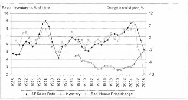
I. Introduction.

As shown

in Figure 1 below, there isa strongpositive correlation

between

housingsales(expressedas a percentofall

owner

households) andthe

movement

in housing prices (R"=.66).

On

the surfacethe relationship looksto be closeto

contemporaneous.There is also a

somewhat

lessobviousnegativerelationship

between

pricesand the shorter series on the inventory of

owner

units for sale(R"=.51).

A

number

ofauthorshaveoffered explanations forthese relationships, in particular that

between

pricesand sales.

Figure 1:

US

Housing

Sales,Prices,

Inventory

Sales,Inventoryas

%

ofstock 10

ChangeInrealsf price,

%

12

aD^~^-r^r^r^oooooooococj)a)cj)aiai

o

o

o

o

o

o

o

o

o

o

CNJ CM CN CM CNJ

-SFSalesRate Inventory -^"—RealHousePricechiange

In one camp,there is a

growing

literature of

models

describing

home

owner

"churn" inthe presenceofsearch frictions

[Wheaton

(1990),

Berkovec

and

Goodman

(1996).

Lundberg

and Skedinger (1999)]. Inthese models, buyers

become

sellers

-

there

are no entrants or exitsfrom themarket. In such a situation the roleofprices is

complicatedby the factthat ifparticipants pay higherprices, theyalso receive

more upon

sale. It isthe transaction cost of

owning

2

homes

(duringthe

moving

period)thatgrounds

prices. Ifprices are high, thetransaction costs can

make

trading expensive

enough

to

almost inverselyto expected salestimes

-

equal to the vacant inventory divided

by

the

sales flow. In thesemodels, boththe inventory and saleschurn are exogenous. Following

Pissarides (2000) ifthe

matching

rate is

exogenous

or alternativelyofspecificform, the

sales timewill be shorterwith

more

saleschurn andprices therefore higher.

Hence

greater salescausehigherprices. Similarly greater

vacancy

(inventory) raises salestimes

and

causes lowerprices.

There are also a seriesofpapers

which

proposethat negativechanges in prices will subsequentlygenerate lowersales volumes. This again isa positiverelationship

between

the

two

variables, butwith oppositecausality.

The

firstofthese is by Stein

(1995) followed by

Lamont

and Stein (1999) andthen

Chan

(2001). Inthese models,

liquidityconstrained

consumers

are again

moving

from one house toanother ("churn")

and

must

make

a

down

payment

in orderto purchase housing.

When

pricesdecline

consumer

equitydoes likewise and fewer households

have

theremaining

down

payment

to

make

the lateral

move.

As

prices rise, equity recoversand so doesmarket liquidity.

Relying instead on behavior economics,

Genesove

and

Mayer

(2001) and then Englehardt (2003)

show

empiricallythat sellers

who

would

experience a loss ifthey sell set higher reservations than those

who

would

not experience a loss.

With

higher reservations, the

marketasa

whole would

see lower salesif

more

and

more

sellers experience loss

aversion as pricescontinueto drop.

In this paper

we

tryto unravel therelationship

between

housing prices and housing sales,and in addition,the housing inventory. First,

we

carefully

examine

gross

housing flows in the

AHS

forthe 11 (odd) years in

which

thesurvey is conducted.

We

find the following.

1). There generallyare

more

purchases of

homes

by

rentersor

new

households

than there are

by

existingowners.

Hence

the focus in the literature on

own-to-own

trades

does;7o/ characterizethe 7?zo/'077(yof housing salestransactions.

2).

The

yearly

change

in the

homeownership

rate is highly correlated negatively

with housingprices. In years

when

prices are high, flows into renting

grow

fasterthan

flows into

owning

and

homeownership

startsto decline.

When

prices are low, net

3).

We

also

examine which

flows addto the inventoryoffor-sale units (called

LISTS)

and

which

subtract (called

SALES). Own-to-own

moves, for

example

do both.

We

show

thatthe

movements

in inventoryare also positively correlated with price.

When

prices are high

LISTS

increase relativeto

SALES,

the inventory grows,and

when

prices

are low, the reversehappens.

4). This leads usto hypothesize thatthere isjointcausality

between

salesand

prices.

Owner

churn generatesa positive schedule

between

sales and prices assuggested

by

frictional markettheory.

At

the

same

time, inter-tenure transitionsshould leadto a

negative schedule.

Along

the latter,

when

prices are high salesdecrease, listsincreaseand

the inventory starts to grow. Inequilibrium, the overall housing marketshould rest at the

intersection ofthese

two

schedules.

To

test these ideas

we

assemble a

US

panel database of101

MSA

across 25

years. This datais from the

NAR

and

OFHEO.

The

NAR

inventory data is tooscattered

and short tobe included in thepanel so our empiricsare limited totestingjust the

hypothesized relationships

between

salesand prices.

Here

we

find:

5). Usinga

wide

range of

model

specifications andtestsofrobustnesshousing

salesjC>o.s77/'ve/)'"Granger cause" subsequent housing price

movements.

Thisreinforces

the relationship posited in frictional search models.

6). There is equally strong empirical support

showing

that pricesnegatively

'Granger cause" subsequent housingsales. This relationship is exactlythe oppositeof

that posited bytheories ofliquidity constraints and loss aversion, but is consistent with

our hypothesis regarding inter-tenurechoices.

Our

paper is organized as follows. Insection II

we

setup an accounting

framework

for

more

completelydescribing grosshousing flows fromthe 2001

AHS.

This involves

some

careful assumptionsto adequately

document

the

magnitude

ofall the

intertenure flows relativetowithin tenure churn and to household creation/dissolution. In

Section 111,

we

illustratethe relationships

between

these flowsand housingpricesusing

the 1 1 years for

which

the flow calculationsare possible.

We

alsopresentour

hypothesized pair ofrelationshipsbetween sales and prices as well asthe relationshipof

eachto thehousing inventory. In sections IV through VI

we

present our empirical

from

1982-2006. It ishere

we

findconclusive evidence thatsales positively"Granger cause"prices andthat pricesnegatively

"Granger

cause" sales.

Our

analysis is robustto

many

alternative specificationsand

subsample

tests.

We

conclude with

some

thoughts

about futureresearch aswell astheoutlook for

US

house prices and sales.

II.

US

Gross

Housing

Flows: Sales,Lists,

and

theInventory.

Much

ofthe theoretical literatureon sales and prices investigates

how

existing

homeowners

behave

as theytry

and

sell theircurrent

home

to purchasea

new

one.This flow is

most

often referred to as "churn".

To

investigate

how

important arole "churn"

plays in the ownership market,

we

closely

examine

the2001

American Housing

Survey.

In "Table 10"ofthe Survey, respondentsare asked

what

thetenure

was

ofthe residence previouslylived in

-

forthosethat

moved

duringthe lastyear.

The

total

number

of

moves

in thisquestion isthe

same

asthetotal in"Table 11"

-

asking aboutthe previous

status ofthe current head(the respondent). In "Table 11" itturns out that

25%

ofcurrent

renters

moved

from

aresidence situation in

which

they

were

notthe head (leaving

home,

divorce, etc.).

The

fraction is asmaller

12%

forowners.

What

ismissing is the joint

distribution

between

moving

by the headand

becoming

ahead.

The

AHS

isnotstrictly

ableto identify

how many

current

owners

moved

either a)

from

anotherunitthey

owned

b) anotherunitthey rented orc) purchased ahouseasthey

became

a

new

ordifferent

household.

To

generate the full setofflows,

we

use information in "Table 11" about

whether

theprevious

home

was

headed

by

the current head, a relativeoracquaintance.

We

assume

that all current

owner-movers

who

were

also

newly

created households-

_were

counted in"Table 10" as previousowners. Forrenters,

we

assume

that all renter-movers

that

were

also

newly

created households

were

counted in "Table 10" in proportion to

renter-owner households inthe full sample. Finally,

we

use the

Census

figures thatyear

forthe net increase in eachtype ofhousehold and fromthat and the data

on

moves

we

are

able to identify household"exits" by tenure.Gross household exitsoccur mainly through

deaths, institutionalization (such as to a nursinghome), or marriage.

Focusingonjustthe

owned

housing market,the

AHS

also allowsusto account

LISTS)

and allofthose transactions that

remove

houses from the inventory (herein called

SALES).

There are

two

exceptions.

The

first is the net deliveryof

new

housing units. In

2001 the

Census

reports that 1,242,000total units

were

deliveredto the for-salemarket. Since

we

have nodirect countofdemolitions

we

usethat figure also as netand it is

countedas additional

LISTS.

The

second is the netpurchases of2"'^ _homes,

_which

count

asadditional

SALES,

butabout

which

there is simply littledata"". In theory,

LISTS

-SALES

should equal the

change

in the inventoryofunits forsale.

These

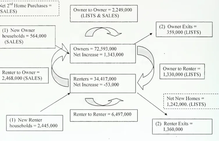
relationships are

depicted in Figure 2 and can be

summarized

with the identities

below

(2001 values are

included).

SALES

= Own-to-Own +

Rent-to-Own

+

New

Owner

[+ 2"^*

homes]

=

5,281,000

LISTS =

Own-to-Own +

Own-to-Rent

+ Owner

Exits

+

New

homes =

5,179,000

Inventory

Change =

LISTS

-

SALES

Net

Owner

Change =

New

Owners

-

_Owner

Exits

+ Rent-to-Own

-

_Own-to-Rent

Net

Renter

Change =

New

Renters

-

RenterExits

+ Own-to-Rent - Rent-to-Own

(1)

The

only other comparabledata is fromthe National Association ofRealtors

(NAR).

and it reports that in 2001 the inventory ofunits for sale

was

nearly stable.

The

NAR

however

reports ahigher level ofsales at 5,641,000. This

7%

discrepancy could be

explained by repeat

moves

within a

same

year since the

AHS

asks only aboutthe

most

recent

move.

It could also represent significant 2"

_home

sales

which

again are not part of

the

AHS

move

data.

What

is

most

interesting to us is that almost

60%

of

SALES

involvea buyer

who

isnot transferring ownership laterally from one houseto another.

So

called"'Churn" is

actually ami)writyofsalestransactions.

These

various inter-tenure sales also are the

criticaldeterminants ofchange-in-inventory since"Churn'" salesdo not affect it. .

Thegroulh instockbetween 1980-1990-2000 Censusesclosely matchessummed completions suggesting

negligibledemolitionsoverthosedecades.The samecalculationbetween 1960 and 1970howeversuggests

removal of3 millionunits.

"_{Net second homepurchases might beestimatedfromtheproduct}

of: theshareoftotal grosshome

purchasesthataresecondhomes(reportedby Loan Performanceas 15.0%) andthe shareofnew homes in

total homepurchases(Census,25%).This wouldyield3-4%oftotaltransactionsorabout200,000units.

Figure

2:

US

Housing

Gross Flows

(2001)

ind

Net

2

Home

Purchases

(SALES)

(1)

New

Owner

households

=

564,000

(SALES)

Renterto

Owner

=

2,468.000

(SALES)

(1)

New

Renter households

=

2,445,000

Owner

to

Owner

=

2,249,000

(LISTS

&

SALES)

Owners =

72,593,000

Net

Increase

=

1,343.000 Renters

=

34,417,000

Net

Increase

=

-53,000 Renterto Renter

=

6,497,000 (2)

Owner

Exits

=

359.000

(LISTS)

Owner

toRenter

=

1,330.000

(LISTS)

Net

New

Homes =

1,242,000.

(LISTS)

(2) Renter Exits

=

1,360,000

Most

inter-tenure

SALES

would seem

to beevents that one might expect tobe

sensitive (negatively) to housing prices.

When

prices arehigh

presumably

new

created

owner

household formation is discouraged orat least deflected into

new

renterhousehold

formation. Likewise

moves

which

involve changes intenure

from

rentingto

owning

also

should be negatively sensitive tohouseprices.

Both

resultbecause higherpricessimply

make

owning

a house lessaffordable.

At

thistime

we

are agnostic about

how

net 2"

home

salesare related to prices.

On

the other sideof Figure 2,

most

ofthe events generating

LISTS

should beat

least

somewhat

positively sensitive toprice.

New

deliveries certainlytryto occur

when

to"cashout",

consume

equityor otherwise switch to renting.

At

thistime

we

are still

seeking a directdatasource

which

investigates in

more

detail

what

events actually

generatetheown-to-rent moves.

Thus

the flows in andoutof

homeownership

inFigure 2 suggestthat

when

prices are high sales likely decrease, lists increaseand the inventory

grows.

These

events

would

easily generatea

downward

sloping schedule

between

prices

and sales such asdepicted in Figure 3

below -

in

compliment

tothe

upward

schedule

developed bytheorists for

owner

occupied churn. Figure 3 presentsa

more

complete

picture ofthe housing market than the models ofStein,

Wheaton,

or

Berkovec

and

Goodman

-

since itaccounts forthe very large roleofinter-tenuremobilityaswell as for

owner

churn.

FIGURE

3:

Housing

Market

Equilibriuni(s)

Search Based Pricing

(own-to-own "churn")

3 o

Pricingbased Sales

{Inter-tfriurcclioiccs)

Sales/Inventory

III.

Further

AHS

Empirical

Analysis.

Unfortunately the gross flows in Figure 2can only be assembled forthe 1 1 years

2007." In

Appendix

III

we

present all ofthecalculated flows foreach ofthese 1 1 years

along withthe

OFHEO

price index.

The

number

of timeseries observationsis not

much

to

work

with so instead

we

just illustrate

some

graphs. In Figure4,

we

show

houseprices against thecalculated

change

in inventory. This is

LISTS-SALES

where

each ofthese is

calculated using the setofidenties in (1). There is a strong positive relationship [R"=.53].

When

prices are high

LISTS

rise,

SALES

fall and the inventorygrows.

Figure

4: Pricesversus

Inventory

Change (LISTS-SALES)

year

Inventorychange •_PriceIndex

InFigure 5,

we

examine

the percentage

change

inthe

number

ofrenters and

owners

ineach ofthe 11 years

-

again with respect to prices.

Here

there is an inverse relationship

between

pricesand the increase in

owners

[R"'=.48] and a positive

relationship

between

prices andthe increasein renters [R~=.29].

When

prices are high, the

number

ofrenters

seems

torise relative to

owners

and theopposite

when

prices are

low.

Thus

there is aparallel negative relationship

between

pricesand the

change

in the

Prior to 1985, the

AHS

useddifferentdefinitionsofresidence,headshipandmoving,sothesurveysare

notcomparable withthemorerecentdata.

homeovvnership rate.

While

these correlations are based on only 11 observations

-

they at

leastspan a longer22 year period.

Figure5: Pricesversus

Tenure

Changes

1985 1987 1989 1991 1993 1995 1997 1999 2001 2003 2005 2907

•ChangeOwners ChangeRenters PriceIndex

IV.

Metropolitan

Sales

and

Price

Panel

Data.

To

more

carefully studythe relationship(s) between housing salesand housing

prices

we

have assembled a large panel data base covering 101

MSA

and the years 1982

through 2006."*

While

far

more

robustthan an aggregate

US

time series, examining

""There have beenafewrecentattemptstestwhetherthe relationship betweenmovementsinsales

and pricessupport one. orthe other, orboth theories described previously.Leung,Lau.andLeong(2002)

undertakeatime seriesanalysisofHong KongHousingand concludethatstrongerGrangerCausalityis

foundforsalesdrivingprices ratherthanpricesdrivingsales. AndrewandMeen(2003) examinea

UK

Macrotimeseriesusinga

VAR

model and concludethattransactionsrespondtoshocksmorequicklythan prices,butdonot necessarily"GrangerCause"priceresponses. Bothstudiesarehamperedby limited observations.

annual dataatthe metropolitanlevel does

have

a limitation, however, since itcannot use

Census

or

AHS

data.

The

latter contain

more

detail aboutthesources ofsalesand

moves,

but the

Census

isavailableonly every decade and the

AHS

sample isjusttoosmall to

generate

any

reliable flowsatthe

MSA

level.

Forsales data, the onlyother consistent source isthatprovided

by

theNational

Association ofRealtors

(NAR).

The

NAR

data isforsingle family unitsonly (itexcludes

condominium

sales in the

MSA

series), but is available foreach

MSA

overthe full period

from 1980 to 2006.'

To

standardize the sales data,

raw

sales

were

compared

with annual

Census

estimates ofthe

number

oftotal households in those markets. Dividingsingle

family sales

by

total households

we

get avery crude sales rateforeach market. In

1980

thiscalculated sales ratevaried

between

1.2%

and

5.1%

across ourmarketswith a

national average valueof 2.8%.

By

contrast, inthe 1980census,

8.1%

of

owner

occupied householdshad

moved

in duringthe lastyear.

By

2000,the ratioofnational

NAR

single

familysales tototal households

had

risen to4.9%, while the

Census

owner

mobility rate just inched

up

to 8.9%.

Of

course our crude calculated averagesales rates should always be lowerthan thecensus reported

owner

mobility ratessince the former excludes

condo

transactionsand non-brokered sales. In addition

we

are dividing

by

total households

ratherthanjust single family

owner-occupied

households. Separate renter/ovv'nersingle

familyhousehold seriesatyearly

frequency

are not available for all metropolitan markets.

The

price data

we

use isthe

OFHEO

repeat sales series [Baily,

Muth,

Nourse

(1963)]. Thisdata series has recently been questioned fornot factoring out

home

improvements

or maintenance and for not factoring in depreciation and obsolescence

[Case, Pollakowski,

Wachter

(1991), Harding, Rosenthal. Sirmans(2007)].

These

omissions could generatea significantly bias in the long term trend ofthe

OFEHO

series.

Thatsaid

we

are left with

what

is available, and the

OFHEO

index isthe

most

consistent

series availablefor

most

US

markets overa long timeperiod.

The

only alternative is to

purchase similar indices from

CSW/FISERV,

although they have

most

ofthe

same

methodological issues as the

OFHEO

data.

'

NAR

_{dataontheinventory ofunits for sale isshorter,andavailableonlyforonly asmallersample of}

largermetropolitanareas.Hence

we

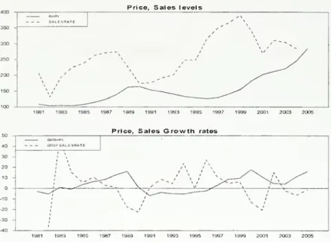
excludeitfromtheanalysis.

In Figures 6 and 7

we

illustratetlieyearly

NAR

sales ratedata, alongwith the

constant dollar

OFHEO

price series

-

both in levelsand differences- for

two

marketsthat

exhibit quite varied behavior,Atlantaand

San

Francisco.

Over

this time frame, Atlanta's

constant dollar prices increase very littlewhile

San

Francisco's increasedalmost

200%.

San Francisco prices, however, exhibitfar greater pricevolatility. Atlanta's averagesales rate is close to

4%

and roughly doubles over 1980-2006. while San Francisco's isalmost

halfofthat (2.6%) and increases

by

only about

50%. These

trends illustrate the topical

range ofpatterns seen across our sample of101 metropolitan areas. In appendix I

we

presentthe

summary

statisticsfor each market's price and sales rate series. Invirtually all markets there is a long term positive trend in the salesrate, as well as in real house prices.

Figure

6: Atlanta Sales, Prices

700

Prico, Sales levels

_ RHP> , - SALESRATE /

.y~"

"

500 ' 400 ' ^ ^ ~-" \ ^ ' ,,

'"

/ 300 -\/ \" 200 -1981 1983 1985 1987 1989 1991 1993 1995 1997 1999 2001 2003 20O5

Price, Sales Growth rates

GHHMPI GRSF SALESRATE 2 -'-.

r\

,-.^ ,-, ;--. r— ^^"^ ^^"--^ ', 2 -,' M -,' 1981 1983 1335 1987 1989 1991 1993 1995 1997 1999 2001 2003 2006 13

Figure

3:

San

Francisco Sales, Prices

400 Price, Sales lovels

RHP. ^v - SALESRATE _{^ ' \} / \ 300 250 \ / \^

"y

200 /

\_

^ '' ' 150 1QO '''

__^

^

^

^^-^

1981 1983 1985 1987 1989 1991 1993 1995 1997 1999 2001 2003 2005

50 Price, SalesGro wth rates GRRHPI 40 ORSFSA LESRATE 30 \ 20 10 ;

'>^-<r^

\ -'""^'' \ '

>

/

/^

_\^

x,^

; ^^ X s * -10 20 ^' -30 "

—

1981 1963 1985 1987 1989 1991 1993 1995 1997 1999 2001 2003 2005

Given

the persistenttrends in both series it is importantto test

more

formally for

series stationarity.

There

are

two

tests available foruse with panel data. In each,the null

hypothesis isthat allofthe individual series haveunit roots and are

non

stationary.

Levin-Lin (1993) and Im-Persaran-Shin (2002) both developa test statistic forthe

sum

or

averagecoefficient ofthe lagged variable ofinterest

-

across the individuals(markets) within the panel.

The

null isthatall ortheaverage ofthese coefficients is not

significantly different

from

unity. In Table 1

we

reportthe results ofthistest for both

housingprice and sale rate levels, aswell as a2"*^ orderstationarity test forhousing price

and sales ratechanges.

RHPI

(Augmented

by 1 lag)

T.4BLE

1: Stationarit> tests

Levin

Lin's Test

Coefficient

T

Value

T-Star

P>T

Levels -0.10771 -18.535 0.22227 0.5879

First Difference -0.31882 -19.822 -0.76888 0.2210

IPS

test

T-Bar

W(t-bar)

P>T

Levels -1.679 -1.784 0.037

FirstDifference -1.896 -4.133 0.000

SFSALESRATE

(Augmented

by 1 lag)

Levin

Lin's

Test

Coefficient

T

Value

T-Star

P>T

Levels -0.15463 -12.993 0.44501 0.6718

First Difference -0.92284 -30.548 -7.14975 0.0000

IPS

test

T-Bar

W(t-bar)

P>T

Levels -1.382 1.426 0.923

First Difference -2.934 -15.377 0.000

With

the Levin-Lintest

we

cannotreject the null (non-stationarity) for either

house price levelsor differences. In terms ofthe sales,

we

can reject the null for

differences in sales rate, but not for levels.

The

IPS test (which is argued tohave

more

power)rejectsthe null forhouse price levels and differences andfor sales rate

differences. In short, both variables

would seem

to be stationary in differences, butlevels

are

more

problematicand likely non-stationary.

V.

Panel

Estimations.

Our

panel approach usesa

well-known

application of Granger-typeanalysis.

We

willask

how

significant lagged sales are in a panel

model

ofprices

which

uses lagged

pricesandthen several conditioningvariables.

The

conditioning variables

we

choose are

marketarea

employment,

andnational

mortgage

rates.

The companion model

is toask

how

significant lagged prices are ina panel

model

ofsales using lagged sales andthe

same

conditioningvariables. Thispair of

model

is

shown

(2)-(3).

P,.r

=

_"o

+

_^\^,:i-\

+

'*2'^/.7-i

+

P''"^i.T

+

S,

+

^i,i (2)

s.j

=

ro

+

7,^,.7--,

+

r2P..T-^

+

^'^..T

+

+n,

+

^,,t (3)

In ourcase there is significantconcern about the stationarity ofboth price and

sales rate levels. This

same

concern should not be presentfordifferences.

Hence

we

will

need toestimate the

model

in firstdifferences aswell as levels

-

asoutlined in equations

(4) and (5).'

AP,7.

=a^+

a^AP,J_,

+

a,AS,j_,

+

jB'AX^j

+

+S,

+

s^^ (4)

^..T =

/o

+

rAS,.r-\

+

/2^,,r-i

+

^'^"^..r

+

+n,

+

^,,t (5)

In panel

VAR

models

with individual heterogeneity there exists a specification

issue. Equations (4) and (5) or (2) and (3) will have an errorterm that is correlated with

the lagged dependentvariables [Nickell, (1981)].

OLS

estimation will yieldcoefficients

that areboth biased and also that are not consistent inthe

number

ofcross-section

observations. Consistency occurs only inthe

number

of time series observations.

Thus

estimates and any tests on the parameters ofinterest(thea and

y)

may

not bereliable.

These problems might

not be serious in ourcase since

we

have 26 time series

observations

(more

than

many

panel models).

To

be on the safe side, however,

we

also

estimated the equations following anestimation strategy

by

Holtz-Eakin et al.

As

discussed in

Appendix

II,this

amounts

to using 2-period lagged values ofsales and prices

as instruments with

GLS

estimation. ' _.vv

, ",'

From

eitherestimates,

we

conducta "Granger"causality test. Since

we

are only

testing for a single restriction,the/ statistic is thesquare root ofthe

F

statisticthat

would

be used totest thehypothesis in thepresence ofa longerlag structure (Greene, 2003).

Hence,

we

can simply use a/ test (appliedto theo:, andy^) ^s the check of whether

changes in sales "Granger cause" changes in priceand vice versa.

Intable 2

we

reportthe results ofequations (2)through (5) in each setofrows.

The

first

column

uses

OLS

estimation, the secondthe

Random

Effects

IV

estimates

from

Holtz-Eakin et al.

The

firstsetofequations is in levels, whilethe second setof

rows

reportsthe results using differences. In all Tables, variable

names

are selfevidentand

differencesare indicated with theprefix

GR.

Standard errorsare in parenthesis.

Among

the levels equations,

we

first notice thatthe

two

conditioning variables,

the national

mortgage

rate and local

employment

havethe

wrong

signs in

two

cases.

The

mortgage

interest rate inthe

OLS

price levels equation and local

employment

inthe

IV

*

In (3)and(4)the fixedeffectsarecross-section trends ratherthan cross sectionlevels as in(1)and(2)

sales rateequation are miss-signed.There is alsoan insignificant

employment

coefficient

inthe

OLS

sales rate equation (despite almost

2500

observations).

Another

troublesome

result isthatthe price levels equation has excess

"momentum"

-

lagged prices havea

coefficientgreater than one.

Hence

prices (levels) can

grow

on their

own

without

necessitating any increases in ftindamentals, orsales.

We

suspect that these

two

anomaliesare likely the resultofthe non-stationary featuretoboththe price and sales

series

when

measured

in levels. Interestingly, the

two

estimation techniquesyield quite

similarcoefficients

-

asmight be expected with a larger

number

oftime series

observations.

When we move

tothe resultsofestimating the equations in differencesall of

these issuesdisappear.

The

lagged price coefficients are small so theprice equationsare

stable in the 2"'' degree, and thesigns ofall coefficients are both correct

-

and highly

significant.

As

to the questionofcausality, in every price or pricegrowth equation, lagged

sales or growth in sales is always significantly positive. Furthermore in ever}' salesrateor

growth

in sales rate equation, lagged prices (or itsgrowth) are alsoalways significant.

Hence

there is clear evidenceofjoint causality,butthe effect

of

laggedprices

on

sales is

always

_of

a

negative sign.

Holding

lagged sales (and conditioningvariables) constant, a

yearafterthere isan increase in prices

-

sales fall.

The

isthe oppositeofthat predicted

by theories ofloss aversion or liquidity constraints, but consistent with our hypothesis.

TABLE

2: Sales-Price

VAR

Fixed Effects

E

Holtz-Eakin estimator Levels

Real Price

(DependentVariable)

Constant

Real Price (lag 1)

Sales Rate(lag 1)

Mortgage Rate Employment -25.59144** (2.562678) 1.023952** (0.076349) 333305** (0.2141172) 0.3487804** (0.1252293) 0.0113145** (0.0018579) -1247741** (2 099341) 1 040663** (0.0076326) 2.738264** (0,2015346) -0.3248508** (0.1209959) 0.0015689** (0.0003129) 17

Sales Rate

(DependentVariable)

Constant

Real Price (lag 1)

Sales Rate (lag 1)

Mortgage

Employment

First Difference

GR

Real Price (DependentVariable) Constant

GR

Real Price (Lag 1)

GR

Sales Rate (Lag 1)

GR

MortgageRate

GR

Employment 2.193724** (0.1428421) -0.0063598** (0,0004256) 0.8585273** (0.0119348) -0.063598** (0.0069802) -0.0000042 (0.0001036) -0.4090542** (0.1213855) 0.7606135** (0.0144198) 0.0289388** (0.0057409) -0.093676** (0.097905) 0.3217936** (0.0385593) 1.796734** (0.1044475) -0.0059454** (0.0004206) 0.9370184** (0.0080215) -0.0664741** (0.0062413) -0.0000217** (0,0000103) -0.49122** (0.1221363) 0,8008682** (0.0148136) 0.1826539** (0.022255) -0.08788** (0.0102427) 0.1190925** (0.048072)

GR

SalesRate (DependentVariable) Constant

GR

Real Pnce (Lag1)

GR

Sales Rate (Lag 1)

GR

MortgageRate 0.7075247 (0.3886531) -0.7027333** (0.0461695) 0.0580555** (0.0183812) -0.334504** (0.0313474) 1.424424** (0.3710454) -0.8581478** (0.0556805) 0.0657317** (0.02199095) -0.307883** (0.0312106)

GR

Employment 1.167302** (0.1244199) 1.018177** (0.1120497) ** indicates significance at

5%.

We

have experimented withthese

models

using

more

thana single lag, but

qualitatively the results are the same. In levels, the priceequation with

two

lags

becomes

dynamically stable inthe sensethat the

sum

ofthe lagged price coefficients is less than one.

As

to causal inference, the

sum

ofthe lagged sales coefficients ispositive, highly

significant, and passesthe

Granger

Ftest. Inthe sales rate equation, the

sum

ofthe

two

lagged sales rates is virtually identical to the singlecoefficient

above

andthe lagged price

levels areagain significantly negative (intheir sum). Collectivelyhigher lagged prices

"Granger

cause"a reduction in sales.

We

havesimilar conclusions

when

two

lags are

used inthe differences equations, but indifferences, the 2"''

lag is alwaysinsignificant.

As

a tlnal test,

we

investigate a relationship

between

the

growth

in houseprices

and the levelofthe sales rate. Inthe search theoretic

models

sales ratesdetermine price

levels, but ifprices are slowto adjust, the impactofsales mightbetter

show

up on price

changes. Similarly the theoriesofloss aversion and liquidity constraints relate price

changesto sales levels.

While

the mixing oflevelsand changes in time seriesanalysis is generally not standard,thiscombination ofvariables is also the strong empirical fact

shown

in Figure 1. In Table 3 price changesare tested for Grangercausality againstthe

levelofsales (as a rate).

TABLE

3: Sales-Price

Mixed

VAR

Differences and Levels FixedEffects

_E

_{Holtz-Eakin estimator}

GR

Real Price

(DependentVariable)

Constant

GR

Real Price(lag 1)

Sales Rate(lag 1)

GR

Mortgage Rate

GR

Employment

Sales Rate

(DependentVariable)

Constant

GR

House Price (lag 1)

Sales Rate(lag 1)

GR

Mortgage Rate -6.61475" (0.3452743) 0.5999102** (0.0155003) 1.402352** (0.0736645) -0.1267573** (0.0092715) 0.5059503** (0.0343458) -0.0348229 (0.0538078) -0.0334235** (0.0024156) 1.011515** (0.0114799) -0.0162011** (0.0014449) -1.431187** (0.2550279) 0.749431** (0.0141281) 0.2721678** (0.0547548) -0.0860948** (0.0095884) 0.3678023** (0.0332065) 0.0358686 (0.0026831) -0.0370619** (0.0026831) 1.000989** (0.0079533) -0.0151343** (0.0014294)

GR

Employment 0,0494462** (0.0053525) 0.043442** (0.0049388) indicates significanceat

5%

19

In terms

cf

causality, these resultsare no differentthan the

models

estimated

either in all levels orall differences.

One

yearafter an increase in the levelofsales, the

growth

in houseprices accelerates. Similarly, one year after houseprice

growth

acceleratesthe levelof

home

sales falls (ratherthan rises). All conditioning variables are

significant and correctlysigned and lagged dependentvariables have coefficients less

than one.

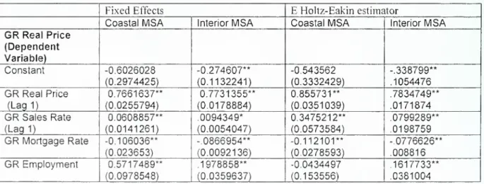
VI. Testsof Robustness,

In panel

models

it isalwaysa

good

ideatoprovide

some

additional testsofthe robustness

of

results, usually by dividing up either the cross section ortimeseries ofthe panel into subsets and

examining

these results as well.

Here

we

perform bothtests. First

we

divide the

MSA

marketsinto

two

groups: so-called "coastal"citiesthatbordereither

ocean, and"interior" citiesthatdo not.

There

are 31 markets in theformergroup and 70 in the latter.

The

coastalcities are often felt tobethose with strong price trends and

possiblydifferent market supply behavior.

These

results are inTable 4.

The

second test is

to divide the sample up by

year-

in this case

we

estimate separate

models

for

1980-1992

and 1993-2006.

The

year 1992 generally

marks

the bottom ofthehousing market from

the 1990 recession.

These

resultsare depicted in Table 5. Both experimentsusejustthe

differences

model

that

seems

toprovide the strongestresuhs

from

theprevious section.

TABLE

4:

Geographic

Sub

Panels

FixedEffects EHoltz-Eakinestimator

Coastal

MSA

Interior

MSA

Coastal

MSA

Interior

MSA

GR

Real Price (Dependent Variable) Constant -0,6026028 (0.2974425) -0.274607** (0.1132241) -0.543562 (0.3332429) -.338799** .1054476

GR

Real Price (Lagi) 0.7661637** (0.0255794) 0.7731355** (0.0178884) 0.855731** (0.0351039) .7834749** .0171874

GR

Sales Rate (Lag 1) 0.0608857** (0.0141261) .0094349* (0.0054047) 0.3475212** (0.0573584) .0799289** .0198759

GR

Mortgage Rate -0.106036** (0,023653) -.0866954** (0.0092136) -0.112101** (0.0278593) -0776626** .008816

GR

Employment 0,5717489** (0.0978548) .1978858** (0.0359637) -0.0434497 (0.153556) .1617733** .0381004

20

GR

Sales Rate (Dependent Variable) Constant 2.098906** (0.7412813) 0.0396938** (0.4541917) 3.03388** (0.7426378) 0.8084169* (0.4261651)

GR

Real Price (Lagi) -0.8320889** (0.0637485) -0 5447358** (0.0637485) -0.9763902** (0.0798291) -0.8519448** (0.0919725)

GR

SalesRate (Lag1) -0.0004387 (0.0352049) 0,0770193** (0.0216808) -0,0350817 (0.0402424) 0.1111637** (0.0251712)

GR

Mortgage Rate -0.2536587** (0.0589476) -0.3772017** (0.0369599) -0.2390963** (00595762) -0.3323406** (0.036746)

GR

Employment 1.265286** (0.2438722) 1.172214** (0.1442662) 1.102051** (0,2223687) 1.03251** (0.1293764) Note: a) *- 10 percent si b)

MSAs

denoted c)

MSAs

denoted

gnificance. **- 5 percent significance.

coastal are

MSAs

near the East or

West

Coast (see

Appendix

I).

interiorare

MSAs

that are not locatedatthe Eastor

West

Coast.

In Table 6,the results of Table4 hold up remarkably strong

when

thepanel is divided by region.

The

coefficientofsales rate (growth)on prices is always significant

although so-called "costal" cities have larger coefficients. In theequationsofprice

(growth) on sales rates, the coefficients are alwayssignificant, andthe point estimates

are very similar as well.

The

negativeeffect ofpriceson sales rates is completely

identical across the regional division ofthe panel sample. Itshould be pointed outthat all

ofthe instruments arecorrectly signed and significantas well.

The

conclusion is the

same

when

thepanel is splitinto

two

periods (Table 5).

The

coefficients ofinterestare significantand ofsimilarmagnitudesacross time periods, and

all instruments aresignificant and correctly signed as well.

The

strongnegative impact of

prices on sales clearlyoccurred during 1982-1992 as well as overthe

more

recent period

from 1993-2006. With fewertime series observations in eachofthe (sub) panels in Table 7, the Holtz-Eakin estimatesare

now

sometimes

quite differentthan the

OLS

results.

TABLE

5:

Time

Subpanels

Fixed Effects

E

Holtz-Eakinestimator

1982-1992 1993-2006 1982-1992 1993-2006

GR

Real Price (Dependent Variable) Constant -2.63937** -0.1053808 -1.237084** -0.2731544 21

(0.2362837) (0.1453335) (0.2879418) (0.1943765)

GR

Real Price (Lag1) 0.5521216'* (0.0271404) 0.9364014** (0.0183638) 0.6752733** (0.0257512) 0.9629539** (0.0196925)

GR

SalesRate (Lagi) 0.0194498** (0.0073275) 0.0363384** (0.0097935) 0.1622147** (0.0307569) 0.0874362 ** (0.0307703)

GR

Mortgage Rate -0.2315352** (0.0193262) -0.0707981** (0.0116032) -0.1432255** (0.0244255) -0.0812995** (0.0163056)

GR

Employment

0.6241497** (0.063533) 0.4310861** (0.0501575) 0.157348* (0.0910416) 0.3441402** (0.0493389)

GR

Sales Rate (Dependent Variable) Constant -6.269503** (0.9018295) 4.398222** (0.447546) -4.898023** (0.8935038) 3.00473** (0.4587499)

GR

Real Price (Lagi) -0.8795382** (0.1035874) -0.5704616** (0.0565504) -1.080492** (0.1243784) -0.4387881** (0.066557)

GR

Sales Rate (Lagi) 0.0056823 (0.027967) -0.025242 (0.0301586) -0.0035275 (0.0350098) 0.066557 (0.029539)

GR

Mortgage Rate -0.5636095** (0.0737626) -0.1934848** (0.0357313) -0.550748** (0.0819038) -0.2720118** (0.0420076)

GR

Employment

2.608423** (0.2424878) 0.4856197** (0.154457) 2.026295** (0.2237316) 0.7631351** (0.1325586) Note:

a)

Column

labeledunder

1982-1992

refertothe results using observationsthatspan

those years..

b)

Coiumn

labeledunder

1993-2006

refer to the results usingobservations thatspan

those years.

VII.

Conclusions

- _

We

have

shown

thatthecausal relationship

from

prices-to-sales is actually

negative

-

ratherthan positive.

Our

empirics arequite strong.

As

an explanation,

we

have

arguedthat actual flows in the housing marketare remarkably large

between

tenure

groups

-

and that a negative price-to-sales relationship

makes

senseas a reflection of

these inter-tenure flows. Higherprices lead

more

householdsto choose rentingthan

owning

and these flows decrease

SALES.

Higher pricesalso increase

LISTS

and sothe

inventory grows.

When

pricesare low, entrantsexceed exits into ownership,

SALES

increase,

LISTS

declineas doesthe inventory.

Our

empirical analysis also

overwhelmingly

supports the positivesales-to-price

relationshipthat

emerges from

search-based

models

of housing churn.Here, a high sales/inventory ratio causeshigher prices and a low ratiogenerateslowerprices.

Thus

we

arrived ata

more

completedescription ofthehousing marketatequilibrium

-

as

shown

with the

two

schedules in Figure 3.

Figure 3 offers a compellingexplanation for

why

in the data, the simple

price-sales correlation is so

overwhelmingly

positive.

Over

timeit

must

bethe "pricebased

sales" schedule thatis shifting up and

down.

Remember

thatthisschedule is derived

mainly from the decision to enteror exittheownership market. Easy credit availability

and lowermortgage rates, for

example would

shift the schedule up (or out). Forthe

same

level of housingprices, easier credit increases the rent-to-own flow, decreasesthe

own-to-rent flow, and encourages

new

households to

own.

Sales

expand

and the inventory

contracts.

The

end result ofcourse is a rise in both prices as well assales. Contracting

creditdoesthe reverse. In the post

WWII

historyof

US

housing, such creditexpansions

and contractions have indeedtended todominate housing market fluctuations [Capozza,

Hendershott,

Mack

(2004)].

Figure 3 also is useful for understandingthe current turmoil in the housing

market.

Easy mortgage

underwritingfrom "subprime capital" greatlyencouraged

expanded

homeownership from

the

mid

1990s through

2005 [Wheaton

and

Nechayev,

(2007)]. This generated an outward shift inthe price-based-salesschedule.

Most

recently,

rising foreclosures have

expanded

therent-to-own flow and shiftedthe"pricebased

sales" schedule back inward. This has decreased both sales and prices. Preventing

foreclosures through creditamelioration theoretically

would

move

theschedule

upward

again, but so could any countervailing policy ofeasing

mortgage

credit. It is interestingto

speculateon whetherthere might be

some

policy that

would

shiftthe"search based

pricing" scheduleupward. This

would

restore prices, although it

would

not increase sales.

For

example

some

policy to encourage interest-freebridge loans

would

certainly

make

it

easierfor

owners

to"churn". Likewise

some

form of

home

sales insurance might reduce

the riskassociated with

owning two

homes. That said, such policies

would seem

to be a

less direct

way

ofassistingthemarketversus

some

stimulus tothe"price-based-sales"

schedule.

REFERENCES

Andrew,

M.

and

Meen,

G., 2003,

"House

priceappreciation, transactions and structural

change

in the British housing market:

A

macroeconomic

perspective", RealEstate

Economics,

31, 99-116.

Baiiy, M.J.,R.F.

Muth,

and

H.O.

Nourse, 1963,

"A

Regression

Method

forReal Estate

PriceIndex Construction". Journal

of

the

American

StatisticalAssociation, 58, 933-942.

Beri<ovec. J.A. and

Goodman,

J.L. Jr.. 1996,"Turnover asa

Measure

of

Demand

for

Existing

Homes", Real

EstateEconomics, 24 (4), 421-440.

Case, B., Pollakowski,H., and Susan

M.

Wachter, 1991.

"On

Choosing

among

Housing

Price IndexMethodologies,"

AREUEA

Journal, 19, 286-307.

Capozza,D., Hendershott, P., and Charlotte

Mack,

2004,

"An Anatomy

ofPrice

Dynamics

in Illiquid Markets: Analysis and Evidence from Local

Housing

Markets,"

Real

Estate

Economics,

lil'A, 1-21.

Chan,

S., 2001, "Spatial Lock-in:

Do

Falling

House

PricesConstrain Residential Mobility?",Journal

_of

Urban

Economics,

49, 567-587... • .

Engelhardt, G. V., 2003,

"Nominal

lossaversion, housing equity constraints, and household mobility: evidence fromthe United States."Journal

_of

Urban

Economics, 53

(1), 171-195. v ; .

Genesove, D. and C.

Mayer.

2001, "Loss aversionand sellerbehavior: Evidence

from

the

\\ous,'mgma-rkQX." QuarterlyJournal

of Economics

A\6

{A), \21>l>-\26f).

Greene,

W.H.,

2003,

Econometric

Analysis, (5"^ _{Edition), Prentice Hall,}

_New

_Jersey.

Harding, J., Rosenthal, S., and C.F.Sirmans, 2007, "Depreciation of

Housing

Capital,

maintenance, and house price inflation...".Journal

_of

Urban

Economics,

61,2, 567-587.

Holtz-Eakin. D.,

Newey,

W., and Rosen, S.H, 1988, "Estimating Vector Autoregressions with Panel Data", £co/70777e/;7ca, Vol. 56, No. 6, 1371-1395.

Kyung

So

Im,

M.H.

Pesaran, Y. Shin, 2002, "Testingfor Unit Roots in Heterogeneous

Panels",

Cambridge

University.

Department

of

Economics

Lamont,

O. and Stein, J., 1999, "Leverage and

House

Price

Dynamics

in U.S. Cities."

RAND

Journal

_{of Economics,}

30,498-514.

Levin,

Andrew

and Chien-Fni Lin, 1993, "Unit RootTests in Panel Data:

new

results."

Discussion

Paper

No. 93-56,

Department

ofEconomics, UniversityofCalifornia at San

Diego. .

~

Leung, C.K.Y., Lau, G.C.K. and Leong, Y.C.F.,2002, "Testing AlternativeTheories of

the Property Price-Trading

Volume

Correlation." The Journal

of Real

Estate Research, 23(3). 253-263.

Nickell, S., 1981, "'Biases in

Dynamic

Models

with Fixed Effects," Econowetrica, Vol.

49,No. 6. pp. 1417-1426. --.. ,

_.^-PerLundborg, and Per Skedinger, 1999, "Transaction Ta.xes ina Search

Model

ofthe

Wo\ismgMar\.Qi'\ Journal

of Urban

Economics, ^5,2, l>i5-l>99.

Pissarides, Christopher,2000, Equilibrium

Unemployment

Theory, 2" edition,

MIT

Press,

Cambridge,

Mass.

Stein, C. J., 1995, "Pricesand Trading

Volume

in the

Housing

Market:

A

Model

with

Down-Payment

Effects," The Quarterly Journal

Of

Economics, 1 _10(2), 379-406.

Wheaton,

W.C., 1990, "Vacancy, Search, and Prices in a

Housing

Market

Matching

Model,''Journal

of

Political

Economy,

98, 1270-1292

Wheaton.

W.C.

and

Gleb Nechayev

2008,

"The

1998-2005

Housing

'Bubble' andthe

Current 'Correction': What's differentthis time?"Journal

of

RealEstate Research, 30,1,

1-26.

APPRENDIX

I: Sales,Price

Panel

Statistics Market

Code

Market Average

GRRHPI

(%) Average

GREMP

(%) Average

SFSALES

RATE

Average

GRSALES

RATE

(%) 1 Allentown* 2,03 1.10 4.55 4.25 2 Akron 1.41 1.28 4.79 4.96 3 Albuquerque 0.59 2.79 5.86 7.82 4 Atlanta 1.22 3.18 4.31 5.47 5 Austin 0.65 4.23 4.36 4.86 6 Bakersfield* 0.68 1.91 5.40 3,53 7 Baltimore* 2.54 1.38 3,55 4,27 8 Baton

Rouge

-0.73 1.77 3,73 5,26 9

Beaumont

-1.03 0.20 2.75 4,76 10 Bellingham* 2,81 3.68 3.71 8.74 11 Birmingham 1.28 1.61 4.02 5.53 12 Boulder 2.43 2.54 5.23 3.45 13 BoiseCity 0.76 3.93 5.23 6.88 14 Boston

MA*

5.02 0.95 2.68 4.12 15 Buffalo 1.18 0.71 3.79 2.71 16 Canton 1.02 0.79 4.20 4.07 17 Chicago IL 2.54 1.29 4.02 6.38 18 Charleston 1.22 2.74 3.34

689

19 Charlotte 1.10 3.02 3.68 5.56 20 Cincinnati 1.09 1.91 4.87 4.49 21 Cleveland 1.37 0.77 3.90 4.79 22

Columbus

1.19 2.15 5.66 4.61 23 Corpus Christi -1.15 0.71 3.42 3.88 24 Columbia 0.80 2.24 3.22 5.99 25 Colorado Springs 1.20 3.37 5.38 5.50 26 Dallas-Fort Worth-Arlington -0.70 2.49 4.26 4.64 27 Dayton

OH

1.18 0.99 4.21 4.40 28 Daytona Beach 1.86 3.05 4.77 5.59 29 Denver

CO

1.61 1,96 4,07 5.81 30 Des Moines 1.18 2,23 6.11 5.64 31 Detroit Ml 2.45 1.42 4.16 3.76 32 Flint 1.70 0.06 4.14 3.35 33 FortCollins 2.32 3.63 5.82 6.72 34 Fresno

CA*

1.35 2.04 4.69 6.08 35 Fort

Wayne

0.06 1.76 4.16 7.73 36 Grand Rapids Ml 1.59 2,49 5.21 1.09 37 Greensboro

NC

0.96 1,92 2.95 7.22

26

38 Harrisburg

PA

0.56 1.69 4.24 3.45 39 Honolulu 3.05 1.28 2.99 12,66 40 Houston -1.27 1.38 3.95 4.53 41 IndianapolisIN 0.82 2.58 4.37 6.17 42 Jacksonville 1.42 2.96 4.60 7.23 43 KansasCity 0.70 1.66 5.35 5.17 44 Lansing 1.38 1.24 4.45 1.37 45 Lexington 0.67 2.43 6.23 3.25

46 Los Angeles

CA*

3.51 0.99 2.26 5.40

47 Louisville 1.48 1.87 4,65 4,53 48 Little Rock 0.21 2.22 4.64 4.63 49 Las

Vegas

1.07 6.11 5.11 8.14 50

Memphis

0.46 2.51 4.63 5.75 51 Miami FL 1.98 2.93 3.21 5,94 52 Milwaukee 1.90 1.24 2.42 5,16 53 Minneapolis 2.16 2.20 4.39 4.35 54 Modesto* 2.81 2.76 5.54 7.04 55 Napa* 4.63 3.27 4.35 5.32 56 Nashville 1.31 2.78 4.44 6.38 57

New

York* 4.61 0.72

234

1 96 58

New

Orleans 0.06

052

2.94 4.80 59

Ogden

0.67 3.25 4.22 6.08 60

Oklahoma

City -1.21 0.95 5.17 3.66 61

Omaha

0.65 2.03 4.99 4.35 62 Orlando 0.88 5.21 5.30 6,33 63 Ventura* 3.95 2.61 4.19 5,83 64 Peoria 0.38 1.16 4.31 6,93 65 Philadelphia PA* 2.78 1.18

352

2.57 66 Phoenix 1.05 4.41 4.27 7.49 67 Pittsburgh 1.18 0.69 2.86 2.75 68 Portland* 2.52 2.61 4.17 7.05 69 Providence*

482

0.96 2.83 4.71 70 Port SL Lucie 1.63 3.59 5.60 7.18 71 Raleigh

NC

1.15 3.91 4.06 5.42 72

Reno

1.55 2.94 3.94 8.60 73 Richmond 1.31 2.04 4.71 360 74 Riverside* 2.46 4.55

629

5.80 75 Rochester 0.61 0.80 5.16 1.01 76 Santa Rosa* 4.19 3.06

490

2.80 77 Sacramento* 3.02 3.32 5.51 4.94

78 San FranciscoCA*

423

1.09

261

4.73

79 Salinas* 4.81 1.55 3.95 5.47 80

San

Antonio -1.03 2.45 3.70 5.52 81 Sarasota 2.29 4.25 4.69 7.30 82 Santa Barbara* 4.29 1.42 3.16 4.27 83 Santa Cruz* 4.34 2.60 3.19 3.24 84

San

Diego* 4.13 2.96 3.62 5.45 85 Seattle* 2.97 2.65 2.95 8.10 86 San Jose* 4.34 1.20 2.85 4.55

87 SaltLakeCity 1.39 3.12 3.45 5.72

88 St. Louis 1.48 1.40 4.55 4.82

89

San

Luis Obispo* 4.18 3.32 5.49 4.27

90 Spokane* 1.52 2.28 2.81 9.04 91 Stamford* 3.64 0.60 3.14 4.80 92 Stockton* 2.91 2.42 5.59 5.99 93

Tampa

1.45 3.48 3.64 5.61 94 Toledo 0.65 1.18 4.18 5,18 95 Tucson 1.50 2.96 3.32 8.03 96 Tulsa -0.96 1.00 4.66 4.33 97 Vallejo CA* 3.48 2.87 5.24 5.41 98 Washington

DC*

3.01 2.54 4.47 3.26 99 Wichita -0.47 1.43 5.01 4.39 100

Wnston

0.73 1.98

292

5.51 101 Worcester* 4.40 1.13 4.18 5.77

Notes:Table provides theaverage real price appreciation overthe25 years,

average job growth rate, averagesalesrate, and growth in sales rate. ;

*

_Denotes

_"Costal city" in robustness tests.

APPENDIX

II

Let A/7,.

=

[zip,./.,....,zVP^y]'and As-,.

=

[A5'|./.,....,z\5';^j.] ',

where

iVis the

number

of

markets. Let W-,.

-

[e,Apy_,,zlSy^,,,A.^,

^

]be the vectorofright

hand

side variables,

where

e is avector ofones. Let F, _{=[s^J.,...,£.^,]}

betheA^x

1 vectorof transformed

disturbance terms. Let

5

=

[aQ,a^,a2,J3^,S^]' _be

thevector ofcoefficients for the

equation. ,- ; -

_.—

Therefore,

Apr

=^^/5 +V^

. (1)

'

Combining

all theobservations foreach time period intoa stacl<; ofequations,

we

have,

Ap

=

WB

+

V.

(2)

The

matrixofvariablesthat qualify for instrumental variables in period

T

will be

Zj^ =[e,ApT^-,,As,_,,AX,j], (3)

which

changes with T.

To

estimate B,

we

premultiply (2) byZ' to obtain

Z'Ap^Z'WB

+

Z'V

.

(4)

We

then forma consistent instrumental variables estimatorby applying

GLS

to equation

(4),

where

the covariance matrix Q.

= E{Z'VV'

Z] .

Q

is not

known

and has to be

estimated.

We

estimate(4) foreach time period and form the vectorofresiduals foreach

period and form aconsistentestimator,

Q

, for

Q

.

5

,the

GLS

estimatorofthe

parametervetor, is hence:

B

=

[W'Z{Q.y'Z'WY'W'Z(Q.y'Z'Ap.

(5)

The

same

procedure appliestothe equation wherein Sales (S)are on the

LHS.

APPENDIX

III:

AHS

Data

(House

Price

Data from

Census)

year 138S 1937 1989 1991 1993 1995 1997 1999 2001 20CB 2005 2007 Rchange 1061 300 414 266 616 -312 116 -65 -53 -181 665 952 change 481 1071 1055 7S2 710 1603 1102 1459 1343 776 978 -221 Nev; Qel. 1072.5 1122.3 1026.3 837,6 1CB9,4 10655 1116,4 1270.4 1241.8 1385,3 1635.9 1216,5 Nev/ 537 553 482 473 557 579 409 430 564 501 641 688 NewR 27H 2877 2751 2381 2725 2959 2377 2387 2445 2403 2507 26SS RR ^25 7438 7563 7485 7184 7714 7494 6934 6497 63 S9 7291 7152 OR 1491 1448 1654 1129 1143 1186 1413 1309 1330 1233 1273 1426 OO IMS 2049 1913 1697 1769 1933 2074 2478 2249 2381 2913 2391 RO 2074 225G 2110 1980 2177 2337 2203 2378 2468 2305 2a)7 2032 Exits S39 295 -117 562 881 127 102 40 359 797 997 1515 RExits 1143 17S9 1881 1764 1075 2120 1465 1333 1360 1512 508 1123

IjsB 520a5 4914,8 4481,3 4225,6 4 S32.4 43S15 47054 5097.4 5179.3 5797.3 eBia9 654aS

Sales laB 4863 4510 4150 4503 4399 4691 5236 5281 S1S7 6161 5111

Price 244.1647 264.3485 27a2473 256.9754 253.5429 253.331 25a1007 274.0435 295.7802 322.0329 37L4579 337,935

RealMedianHouse

PrKB 1454aai 1S621S7 158258.4 1563S4.1 156S7S9 159199.3 166624.9 175750.3 13^404.1 2030625 232526,1 217900