COAL : a continuous active learning system

COAL: A Continuous Active Learning System

by

Jonathan Johannemann

Submitted to the MIT Sloan School of Management

in partial fulfillment of the requirements for the degree of

Master of Finance

at the

MASSACHUSETTS INSTITUTE OF TECHNOLOGY

June 2017

@

Massachusetts Institute of Technology 2017. All rights reserved.

Signature redacted

A u th o r ... . . .. . . .... . ...

MIT Sloan SchoK'o Management

May 26, 2017

Certified by... ...

Signature redacted

I'alyan Veeramachaneni

Principal Research Scientist

Thesis Supervisor

Certified by ...

Accepted by...

Signature redacted

Tauhid Zaman

Assistant Professor

Thesis Supervisor

Signature redacted

Program Director,

JUN 2

2017

MIT

Sloan

ter of Finance Program

w

=

COAL: A Continuous Active Learning System

by

Jonathan Johannemann

Submitted to the MIT Sloan School of Management on May 26, 2017, in partial fulfillment of the

requirements for the degree of Master of Finance

Abstract

In this thesis, our objective is to enable businesses looking to enhance their prod-uct by varying its attributes, where effectiveness of the new prodprod-uct is assessed by humans. To achieve this, we mapped the tast to a machine learning problem. The solution is two fold: learn a non linear model that can map the attribute space to the human response, which can then be used to make predictions, and an active learn-ing strategy that enables learnlearn-ing this model incrementally. We developed a system called Continuous active learning system (COAL).

Thesis Supervisor: Kalyan Veeramachaneni Title: Principal Research Scientist

Thesis Supervisor: Tauhid Zaman Title: Assistant Professor

Acknowledgments

First and foremost, I would like to thank my advisers Kalyan Veeramachaneni and Tauhid Zaman for their support and guidance. Without their help, this thesis would not look the same. When I was overly ambitious, they helped me stay on track and, when I faced a wall, they provided the feedback and process necessary to push me forward. They inspired me and made me realize the thrilling gratification that can come with a career in research. Everything they taught me, I will always carry in the career I make for myself.

I am incredibly grateful for the generous funding support from Coca cola for this research. I'd like to thank the Coca cola team: Xiaorong You, Aaron Woody, Fer-nando Carriedo, Linda Liu, Robert Kriegel, Paul D Winget, for helping us set up this problem, explaining us its different nuances and for the many beneficial discussions over the course of the year.

I'd like to thank all of my colleagues at Data to Al lab for a great year. Their

contagious enthusiasm for building Al systems made the research process all the more enjoyable and exciting. I hope the best for all of them.

Finally, I'd like to thank my brother Steven and my parents for all of their love and support.

Contents

1 Introduction 13

1.1 Active Learning vs. our current scenario . . . . 16

1.2 What are the constraints? . . . . 17

1.3 A continuous active learning system . . . . 18

1.4 Thesis Roadm ap . . . . 19

2 Non-Linear Modeling 21 2.1 Machine Learning Models . . . . 22

2.1.1 Neural Networks . . . . 23

2.1.2 Gaussian Process Classifiers . . . . 23

2.1.3 Modeling with a Human Component . . . . 24

3 Active Learning 27 3.1 Active Learning Methods . . . . 28

3.2 Active Learning Successes . . . . 30

4 COAL: A continuous active learning system 33 4.1 Modeler, Predictor, Proposer Framework . . . . 33

4.2 Running Active Learning Iterations . . . . 34

4.3 COAL User Interface . . . . 36

5 Robustness Experiments 39 5.1 Generating Ground Truth Models . . . . 40

5.2.1 Evaluation Metric: Area under the Accuracy Curve . . . . 46

5.3 Machine Learning Model Selection . . . . 47

5.4 Active Learning Method Selection . . . . 50

5.5 Key Findings . . . . 53

6 Conclusion 55 6.1 Key Findings . . . . 55

6.2 Contributions . . . . 55

List of Figures

2-1 This graphic depicts a basic neural network which takes 3 inputs through the input layer, propagates these inputs through the hidden layer, and

outputs probabilities of each pre-specified class in the output layer. . 23

2-2 This graphic depicts an instance of the type of boundary that Gaussian

Process Classifiers create when fitting data.

ill

5-1 This graphic depicts the performance of area under the accuracy curve

for an experimental run with Gaussian Process Classifiers where one is using smallest margin and the other is using "random". . . . . 46

5-2 This graphic depicts the performance of area under the accuracy curve

for Gaussian Process Classifiers compared to Neural Networks with one

standard deviation bounds . . . . 50

5-3 This graphic displays the average area under the accuracy curve for the

Gaussian Process Classifier and Neural Networks, the corresponding active learning methods, and the one standard deviation above up to

Ground Truth Model Hyperparameter Arguments

Scikit-learn MakeClassification Arguments . . .

ML Model Robustness Test Inputs . . . .

Results from Model Robustness Tests . . . . Active Learning Robustness Test Inputs . . . . . Results for Active Learning Robustness Testing .

List of Tables

Chapter 1

Introduction

Businesses are constantly striving to improve old products or generate new ones. In many industries, performance measures for products are objective: the best graphics card runs the most computations per second, the best database provides the fastest queries, or the best television is the one with the highest definition. In this thesis, we focus on products for which performance is largely subjective: human assessment and preference is required in order to determine the superior product. These assessments can come in the form of a of rating (on a scale of 1 -5), a binary decision (like or dislike) and in some cases judgment as to whether or not a difference is noticeable1. This means that products require an evaluation that is far less mechanical, which makes the feedback and testing processes much more difficult.

The current method of generating new products: We are focused on problems

where industry research departments tinker with multiple variables that make up the product in order to come up with a new one that, when assessed by humans, will surpass their current product in the metric of their choosing. This process relies primarily on the domain expert's knowledge of what may or may not work. The domain expert also has an understanding of the various constraints and underlying properties of the variables he or she has to work with, which could include:

* How variables interact: Some variables may interact with others and create

'This is the case with our sponsor, Coca Cola, where they are trying to find new coatings that do not change a product's flavor profile or taste experience

effects which might be detrimental to the intended goal.

" Sensitivity: Domain experts may have identified weak trends in the inputs and

human responses. Experts may observe x1 ... Xk but notice that in particular,

changes in x1 and x3 are easily noticed by humans.

" Variable limits: Domain experts also know the bounds within which each

of the variable's values should fall. These bounds are often also dictated by

external factors. For example, if it is a product that is consumed, there are certain limits on concentration for a given variable input.

While expert knowledge of variable interactions, sensitivities and constraints is ex-tremely helpful, it still leaves a considerable amount of options for potential new combinations, and it is challenging to search through that space. Below, we describe a few of these challenges.

Challenges in searching through this space: While domain experts can create

a defined feature space and use their prior knowledge to search for new combinations for products, there are limitations to what a business can do:

o Cost: The challenge of cost is broken into the economic costs and time costs that come with running experiments.

Take economic costs: when running an experiment that requires human assess-ment, participants must be paid, and accommodations must be made in order to avoid confounding variables if any exist. Then, experts need to take their combination of inputs and synthesize many instances of the new product in order to get a large enough pool of responses to determine whether the new product is significantly better. All of this can incur a large cost, and must be done at each iteration of product testing.

On top of that, for time costs, each step of the experimentation and human validation process may take a considerable amount of time. Time must be allocated towards generating new products. Additionally, it also takes time to gather a panel of humans to test the product. This results in human capital,

which could otherwise provide benefits to a company in a different function, being locked up in the maintenance and continuation of a project.

9 Domain expert limitations: Because industry scientists cannot try an

end-less number of combinations, they need to intelligently select the few that will give them an idea of what area in their feature space they should look in. However, domain experts are challenged as the dimensionality of the problem increases; that is, the challenge increases along with the number of variables they have to work with. While a domain expert may have intuitions regard-ing interactions among a few variables, and may be able to weakly postulate the human response, making accurate predictions becomes less feasible as the number of variables increases.

A potential solution using machine learning: In order to solve this problem

using machine learning, one could fit a nonlinear model to determine the relationship

between the available variables and the human responses - rating, like or dislike,

judgment, or some other measure that establishes the product's success. Then, in a perfect setting where this relationship is accurately modeled, a user can search for the combination of variable values that results in the best product by predicting the human response using the model, instead of going to humans each time.

However, coming up with this accurate nonlinear model requires multiple steps and iterations.

1. Users must first start with a few data points, which can be sampled randomly

or exist from prior experimentation.

2. Then, the existing few data points must be modeled to get a preliminary non-linear model to work with.

3. From here, a user needs to identify valuable data points to improve the model

via an approach called active learning or data points that will bring them closer

4. The user must then go out and synthesize a product from this combination of data points, and retrieve an aggregate response from a panel of testers.

5. The user then updates their model and repeats the process from step 3 to further

improve their model and sample better products.

Ultimately, the result of this repeated process will create a model that allows a user to identify the best combination of inputs for his or her product without running countless human-in-the loop experiments.

1.1

Active Learning vs. our current scenario

Active learning is a field of study that looks to help researchers identify the data points that will best improve their models if provided labels.

[6]

classification on text data.

[5]

with which to conduct preliminary training of a classifier. Even without a substantial amount of initial data, users can hire mechanical turks and acquire a sizable base to train on for a relatively low cost due to the nature of tagging image data.

From here, users have enough data to begin making predictions on unlabeled data in order to identify the most valuable data for their models using active learning methods. [211 The same is true for sentiment analysis of text data. While there are not as many text datasets with labels, and sentiment analysis does take more time, data labeling can be done remotely in relatively little time. Then, users can repeat the same process of building models and beginning to identify informative unlabeled data for labeling.

In this thesis, we consider a slightly different problem where human assessments cannot be collected remotely or digitally.

Our use case is that of sensory evaluation. In sensory evaluation, humans either taste, smell or touch new products in order to assess them. These new products could involve flavors or fragrances. These experiments require the physical presence of the

human assessor and cannot be done digitally. Additionally, they require much more control than other types of evaluation to avoid erroneous results. In the instance of image classification, external factors such as health, mood, or other sources that can influence a person's subjectivity will not impact a person's ability to recognize objects like a dog in a picture. However, that is not the case in sensory evaluation. The evaluation is often done in a controlled setting to account for environmental factors.

A perfect example is the unique problem provided to us by Coca Cola. Coca Cola

is interested in changing the coatings on the insides of their cans, but they do not want the customer to taste a difference. In similar scenarios where companies are looking to change a consumed product, firms take multiple steps to carefully ensure that there are no confounding variables or measurement errors. Panelists of consumers are brought on-site to avoid confounding variables and are given food to cleanse their pallets after trying each sample, and results are meticulously kept. As one can see, each iteration requires a substantial amount of time for generating new samples and testing, and even with these precautions, a company can only run so many tests before the panelists' sensitivities to taste are potentially dulled. Therefore, our problem is slightly more nuanced than most, and requires further thought before using an active learning solution.

1.2

What are the constraints?

Let us consider, then, the unique hurdles that sensory evaluation presents for the development of an active learning solution.

" We do not have many points to start with. To begin with, we do not

have many data points to develop, test and validate a machine learning model. Without this we cannot start with a non-linear model.

" We cannot ask for more data points. Given the lack of data points, we

however, it is unlikely that we could do so; experiments take time.

Yet our goal is to develop and deliver a machine learning system that is capable of performing the 5 steps mentioned above in the first section under "A potential solution

using machine learning". Hence, we examined: if we were given enough data, what

questions could we ask in order to deliver a good system? There are three questions we would have sought to consider:

1. Which machine learning model best fits the data? There are many

different modeling techniques with different ways of modeling non-linearities. We would have asked which non-linear model best fits this type of data. 2. Which active learning method is best? As with the above, and with a lot

of labeled data, we would have asked which one of numerous techniques would work best for this problem.

3. Does active learning help?: We would have asked whether an active learning

loop would help in this context.

1.3

A continuous active learning system

We thus developed a continuous active learning system (COAL) as an answer to industry's need to navigate unlabeled data efficiently and cost-effectively. We take in all of the considerations and predispositions mentioned above in order to create a system that allows a user to leverage machine learning to model the data that he or she does have and to search this space.

In order to address a lack of data to begin with, we attempt to ensure the ro-bustness of machine learning models and active learning methods chosen to embed in COAL. We run thousands of simulated active learning experiments that test a variety of nonlinear models for a variety of different human assessment functions that we create through "ground truth" models.

determine whether or not active learning will actually help given our problem and, if it does, which methods are the best for this type of learning scenario.

Ultimately, the user is provided the most robust modeling technique as well as an active learning strategy, as assessed from these experiments, that is integrated into a series of modules. These modules allow the user to model their data, predict the response from a combination of inputs, and intelligently propose new queries for labels. This way, after enough initial experimentation and human testing, a user would be able to accurately model the function that drives human assessment and infinitely test new products without the costs that are typically associated with that process.

1.4

Thesis Roadmap

The remainder of the thesis is organized as follows:

Chapter 2 introduces how machine learning is used, one of the major challenges that modelers face, the models we test, and successful use cases.

Chapter 3 talks about how active learning is used, some of the strategies, and past successes.

Chapter 4 discusses the COAL system and its primary components at length, and introduces an end-to-end explanation of its use. Chapter 5 runs through the process of how we go about simulating active learning experiments and the results of these simulations. Finally, Chapter 6 reviews key findings, identifies the core contributions of this work, and provides insight into what future work will look like.

As a whole, this thesis introduces a system for running active learning in non-traditional active learning settings.

Chapter 2

Non-Linear Modeling

One of the core components of the solution is the non-linear model, which is the user's attempt at recreating the actual underlying function that determines a human's response. The non-linear model does what a domain expert cannot by capturing higher-dimensional relationships, and providing a more analytically sound method of making forecasts on the outcomes of testing given a combination of variables. As a result, many companies are currently taking advantage of machine learning in tasks that can be systematically broken down, and where basic human discretion can be substituted with statistical forecasts.

Overview of using machine learning: Many resources have been created that

al-low users to easily train and utilize machine learning models in a variety of languages. The following provides a basic understanding of how machine learning models are built, and how they function:

1. Prior to training: Prior to training, machine learning models comprise a

series of assumptions about the data, adjustable weights or kernels, and an algorithmic framework through which the function inputs pass through.

2. Training the models: Training machine learning models focuses on finding a set of parameter weights that, when combined with the model assumptions

and the algorithmic framework of the model, provide an output close to the actual observed process. This process may be thought of as a user going back

and forth between inputs and outputs by tweaking the weights of the model so that, if the same inputs were ever provided in the future, they would provide the same corresponding outputs.

3. Using the model after training: The primary function of using a machine

learning model after training is to forecast the output of a new set of inputs.

The model selection problem: One of the main problems in machine learning is

determining the model that best captures the relationship between the input variables

X1 ... Xk and the response variable y. These models, to list just a few, include random forests, support vector machines, Gaussian processes, and neural networks, all of which make different assumptions about the data and model the data in substantially different ways. In most modeling scenarios, the user has a sizable pool of data to model from. The benefit of having this pool is that a user can fit a wide variety of models to the data to determine which achieves the best accuracy or is the most robust. A large pool of data allows the user to run various forms of cross-validation, and modelers can use multiple different model selection methods to determine which model is right for the task. Sadly, we do not have a large enough initial pool of data; hence, there is no way for us to explore various models, simply because there will not be enough instances to draw any conclusions with conviction. Therefore, we are required to make different considerations in our model selection process, and run tests as specified in Section 5 in order to choose the most robust model for all cases as opposed to a model that would be a best fit for a given application.

2.1

Machine Learning Models

In this thesis, we focus primarily on two classification methods with the capacity to capture highly non-linear relationships between data points and a response variable. The two models that we focus on are Gaussian process classifiers and neural networks.

output

layer

input layer

hidden layer

Figure 2-1: This graphic depicts a basic neural network which takes 3 inputs through the input layer, propagates these inputs through the hidden layer, and outputs

prob-abilities of each pre-specified class in the output layer.

2.1.1

Neural Networks

Neural networks are a very powerful type of nonlinear classifier that have grown in popularity due to recent strides in areas such as computer vision and natural language processing (we have even found instances in which researchers used neural networks in conjunction with sensory analytics [23]). A neural network is generally characterized

by an input layer, a hidden layer which is its defining feature, and an output layer

where label probabilities are outputted. Another way to think of neural networks is as a series of layered logistic regression functions. At each node of the neural network, multiple inputs are provided and go through a sigmoid function, just as they would in a logistic regression. The difference is that neural networks take the outputs of the initial nodes or sigmoids and use those as inputs to additional logistic regression functions. This ultimately results in a highly nonlinear classifier that is able to capture a variety of different functions.

2.1.2

Gaussian Process Classifiers

The second nonlinear classification model that we consider is the Gaussian process classifier. This model is also able to robustly capture nonlinear relationships. The

0 X9 X

/ 0

0 0 X) X

-2 0 2 -? 0

Figure 2-2: This graphic depicts an instance of the type of boundary that Gaussian Process Classifiers create when fitting data. [1]

Gaussian Process Classifier is non-parametric and specified by its mean function and covariance function. Perhaps one of the easier-to-understand explanations of Gaussian

Processes can be found in Murphy's Machine Learning:~ A Probabilistic Perspective:

A GP defines a prior over functions, which can be converted into a posterior over functions once we have seen some data. Although it might seem difficult to represent a distribution over a function, it turns out that we only need to be able to define a distribution over the function's values at a finite, but arbitrary, set of points, say xi ... XN. A GP assumes that p(f(x1), . .. , f(xN)) is

jointly

covariance Z(x) given by = k(xi, xi), where k is a positive definite

kernel function. The key idea is that if xe and x3 are deemed by the kernel to be similar, then we expect the output of the function at those points to be similar, too.

till

The Gaussian Process is then funneled through a sigmoid function which,

just

as it does in logistic regression, turns the problem from a regression problem into a classification problem.

2.1.3

Modeling with a Human Component

While it may seem overly complicated to model the behavior or abilities of people given that each person is unique, at an aggregate level, scientists have found that there are patterns that persist. Companies such as Netfiix are able to create recommender

systems that identify human preferences and provide suggestions on what the person may want to watch next. [221 Researchers are also capable of identifying the content of images with a high degree of accuracy. [10] What these successes in machine learning mean is that any process can be modeled and to a high degree of accuracy even when something as fickle as a human is involved. However, at the end of the day, these models are only frameworks and are as good as the data they are trained on which brings us to Section 3.

Chapter 3

Active Learning

The active learning problem is best known as a situation where a modeler wishes to identify a relationship between a set of input variables X1 ... Xk and a response variable y but has largely unlabeled data. The alternative scenario is a branch of machine learning called supervised learning where the user receives input values for each variable X1 ... 34 and also receives the actual outputs y for those values. This scenario is far more common because it does not require much discretion in the gathering of data points. However, in active learning, usually due to some cost of labeling or gathering each response value y, researchers attempt to formally capture the relationship with the fewest labels y.

The active learning process: In active learning, the process is composed of two

main constituents: the oracle and the modeler. The oracle is an omniscient labeler who is capable of providing a label for any combination of inputs asked for by the modeler. However, each request for a label comes at some cost. In order to minimize the cost, the modeler uses his or her model that has been trained on the data he or she does have labels for, the unlabeled data, and active learning methods to identify valuable or informative data points. After each query is made to the oracle, the modeler updates the trained model which brings it closer to the true relationship between the input variables and the response variable. From here, the modeler repeats this process to continually improve the accuracy of the trained model.

3.1

Active Learning Methods

There are a wide variety of ways to determine whether a given unlabeled data point is informative. Information can come from the nature of the data itself if there are clusters or certain structures such as multiple levels of clustering. A modeler can also look at the model he or she is using as well to determine what could potentially be helpful for capturing the relationship in the data. He or she could see if the model believes that two classes are equally probable or whether or not updating the model with a given data point and label would reduce the overall prediction error.

The methods that we explore for the COAL system at this current time are pri-marily the single-query methods that are well established throughout active learning literature. They are smallest margin and entropy. These methods are generally well understood and fairly easy to interpret given their simplistic nature. The process to use these methods is as follows:

1. As a modeler, you begin with your labeled data X and labels Y.

11 ... X1N

11

Xiabeled = ... and Yabeled =

XM1 ... XMN

[m

2. You then train your classification model f(x) = y.

3. From here, you predict the probabilities of each class C for all 1 to K classes on

all unlabeled data points.

X11 ... X1N

1[

Xunabeled = : . f(Xunabeled) =

-[XM1 ... XMN [PM(C1) ... PM(CK)J

4. Next, the user can choose to use smallest margin or entropy to determine the next query.

For smallest margin

[14]:

(a) For each row, find the two highest probability values and calculate the difference A between the two values.

(b) Append each delta to a list called Margin.

Margin = [A, ... AM

(c) Now, sort the list from lowest to highest in descending order and select the top query to propose by finding the index corresponding to the actual

combination of inputs x found in Xunlaeled.

For entropy

[19]:

(a) For each row, calculate the entropy of f(Xuniabeled) as enm = EK pmnl0g2(pmn)

(b) Append each entropy value to a list called Entropy.

Entropy = [eni ... enMI

(c) Now, sort the list from highest to lowest in descending order and select the top query to propose by finding the index corresponding to the actual

combination of inputs x found in Xunlabeled.

On a last note, another strategy that we will refer to is the "Random" uncertainty sampling strategy. Random is essentially how supervised learners will sample data or those that use little to no discretion in determining what data is more informative. To use this method, one just randomly selects a data point from the existing data pool. This is what we consider as the benchmark for the efficacy of the active learning strategies.

3.2

Active Learning Successes

In recent years, active learning has grown in popularity due to a widespread interest in determining whether or not machine learning can solve a variety of problems in industry. Some of the potential benefits that users of active learning are looking for are:

" Reduction of Costs: This factor is key, because companies are limited in the

amount of time and money they have to create a new product. Also, there is a competitive edge for those who are able to generate a product faster.

* Training Time Reduction: Although GPU computation has improved

sub-stantially in the last decade, modelers are still looking for means to cut down on the amount of time it takes to train a model. In [211, training a deep neural net for image classification took 17 hours with a Titan X GPU for 44,708 images which was one of the fastest commercial graphics cards available at that time. Even with the computational improvements since then and the ability to run calculations in parallel, researchers are limited in the complexity of the model that they can train. Therefore, modelers are hoping to reduce the training data sets to at least gain some reduction in the amount of computation required in order to achieve the same accuracy results as one would get if training on all of the data available.

" Improving Existing Classifier Accuracy: Finally, a third application for

active learning is also for the sake of further improving models. While many modelers are able to capture the more robust features of the classes that they are trying to identify in image data and so on, their models still tend to suffer in edge cases. This is another area where, even after one has fully trained a model, active learning can still provide a level of benefit by capturing rare or unusual cases to learn a model from.

Proof of Active Learning Success: At this point, active learning has definitively

[21], researchers were able to train a deep learning model with slightly above 60%

of the the CACD dataset

[4]

achieved a similar accuracy rate to a supervised learner who used the entire dataset to train the same model. Then, in [3], researchers used Gaussian mixture models with

active learning on the VidTIMIT [7], a video and audio dataset, and MOBIO [13],

a biometric dataset. In both cases, active learning methods performed much better than the supervised learning benchmark of randomly selecting data points to label. In some cases, the active learning methods allowed the modeler to achieve the same accuracy as the supervised learner but having trained on half the number of data points. There is a great deal of interest in how the data collection process can help researchers create better models with fewer labeled data points.

Chapter 4

COAL: A continuous active learning

system

To reiterate, the problem that COAL aims to tackle is the scenario where a modeler is trying to determine the most informative data points in order to build a model that is representative of the underlying data generating process. This process is generally unknown to the domain expert or user and, at most, users generally have an idea of constraints only but not much more. COAL's objective is to take this problem and map it to a learning problem through the use of active learning strategies and machine learning models. COAL's framework allows users to continually query for data points in order to find informative data points and continuously improve the accuracy and conviction of their models.

4.1

Modeler, Predictor, Proposer Framework

The COAL system has three components.

1. Modeler: The modeler models the latest available data samples. In our case,

these data samples are the input variables x1 ... Xk and the aggregated response

from the human panel. To model this data, we chose two different types of modeling techniques: neural networks and Gaussian process modeling.

2. Predictor: The predictor module allows the user to propose a new combination

of variables and receive two prediction outputs. The first prediction will be the label that the model believes that the data point has and the second value will be the probability that the model assigns to the likelihood of it being the "detected" label.

3. Proposer: Using the active learning methods we developed, the proposer

sug-gests the next combination of input variables to try by proposing attributes, which the user can then experiment with. The proposer uses the latest model and the data from the past experiments to come up with new data to query. The proposer then creates a number of data points by generating values for

attributes X1 ... Xk and by stepping through the multidimensional space with a

step size s. This will create 1-1k1 max(x )-min(xj) possible input combinations.

Next, we pass all these candidates through the up-to-date model. The model, in turn, provides the likelihood probability for each of the input combinations to succeed in human panel testing. Our goal is to pick a candidate from these. In order to maximize exploration of the space, we use two methods such as smallest

margin and entropy to pick a candidate[6]. As a result of querying informative

samples, we have a higher potential for more consistency and improvement in accuracy of our model as new samples are labeled and added to the model.

4.2

Running Active Learning Iterations

Now that we have outlined the core components of the COAL system, we go into detail on how one would run active learning iterations. The COAL system is to be used in the following manner:

1. The user provides preliminary data with labels, model type, and model

hyper-parameters to the Modeler function.

3. The Modeler function creates a "Trained_Model.pkl" file which is saved to the

current working directory.

4. The Modeler function outputs the current model to be used in further compo-nents of the COAL system.

5. From here, users are able to leverage the model to gain access to the predictor

and proposer functionalities and would start with the Predictor function.

6. To use the predictor, the user provides inputs for each variable and then clicks

predict. This allows a user to formulate potential queries and compare with the current model to see if the model agrees with his or her intuition. In many cases, these potential query designs can come from different analytical methods.

7. Now, the user moves on to the Proposer function and provides the trained model

which was created using Modeler, the number of variables, the minimum ranges for each variable, the maximum range values for each variable, the step sizes to be observed between each minimum and maximum value, the active learning method, and the number of queries.

8. The proposer then consists of three sequences that occur in the following order:

(a) The proposer makes a call to an internal function called "Data Generator". The Data Generator function takes the trained model, number of variables, minimum range values, maximum range values, and step sizes in order to generate a range of data point combination defined by the inputted values. For example, if I have 1 variable, a minimum range value of 0, a maximum range value of 10, and a step size of 2, the outputted data will be 0,2,4,6,8,101.

(b) The proposer then has the trained model predict on the entire array of

input values that were created by the Data Generator function. The result of these predictions are a series of probabilities for each provided label class.

(c) Finally, the proposer makes a call to one of the active learning strategy functions depending on the active learning method parameter provided to the proposer function. The active learning function will return informative queries based on the probabilities provided and the number of queries requested.

9. The proposer then outputs the informative samples for the user to take to an

external oracle for the labels to be queried.

10. Once the labels have been identified for the informative samples, the user is to

add these data points along with their labels to the respective input X and label Y arrays.

11. Now, since the data has been updated and there is new data to train on, the user

will once again call Modeler to update the model based on the new information provided.

12. The user repeats steps 6 - 10 continuously in order to further explore the feature

space until generally an external constraint such as an economic stopping criteria is applied.

4.3

COAL User Interface

Additionally, we developed a front end application for users without programming experience to gain access to COAL. The following steps provided will guide a user through the active learning process via this interface. Much of this process is similar to Section 4.2 but with a few nuances that are specific to the user interface. The steps are as follows:

1. The user is prompted for the number of variables which is saved in the back

end.

2. The user is prompted for the variable names to carefully track what values correspond to what ingredients or actual variables in the experiment.

3. The user then goes to the Modeler page which has four different windows. One

for Panelist responses, one for ingredients, one to model the data, and one to download the training data so far.

4. The user clicks on the upload button under ingredients in order to upload an "Ingredients.csv" file.

5. The user clicks on the upload button under the panelist responses in order to

upload a "Panelist Responses.csv" file.

6. Then, the user clicks the "Model" button under the Modeling section. Behind

the scenes, the chi-square test is calculated for the panelist responses to deter-mine the aggregate response of the panelists. Then, the ingredients and aggre-gate responses are joined and appended to the "TrainingDataSoFar.csv". Finally, a model is trained based on the ingredients or variables and the re-sponses in the "Training_ Data_SoFar.csv" file.

7. From here, the user can move on to other modules. Next, a user may proceed

to the Predictor module.

8. The user provides inputs for each variable and then clicks predict. This allows

a user to check to see what the model thinks about various combinations of potential inputs. This stage is where the user can evaluate certain priors based on application based knowledge and further validate or question his or her hypothesis of viable data points to label.

9. Next, the user can go to the Proposer module which will allow him or her to take

advantage of active learning strategies. The user supplies the maximum value constraints, the minimum value constraints, the step size, and active learning method in order to get a proposed combination of variables.

10. The user would then synthesize a product from these combinations of variables

file. Furthermore, the researcher would input the combination of variables into another "Ingredients.csv" file.

11. Finally, the user would go back to the Modeler page and repeat the process from

Chapter 5

Robustness Experiments

In traditional machine learning, data collection is often trivial, and data scientists are able to hire mechanical turks [8] to collect thousands of data points to build initial models. This allows them to try a wide variety of models such as neural networks, random forests, support vector machines, and many more to determine which model is the best for the task at hand. Since we want to address situations with no or minimal data in this thesis, we need to devise a means of testing viable models for robustness so that, when the data is introduced, the model is able to capture all of the underlying nuances and variations.

Second, this relatively substantial pool of initial data also allows the best model to begin to robustly capture some of the underlying relationships in the data. Re-searchers have found that active learning, which tends to focus on unclear or "hard to identify" examples without a base of "easy to identify" data points, can confuse a model into failing to create robust decision boundaries [2]. Therefore, in this section, we also seek to answer whether or not active learning helps in our scenario and, if multiple models are helpful, which one is the most robust.

To answer these questions, we begin by coming up with different variations of nonlinear ground truth models to replicate what the data might look like. In Sec-tion 5.1, we describe the steps necessary to create each ground truth model, and go through what can be varied in the process. Then, in Section 5.3, we address the ma-chine learning model selection process. In this section, we select a model, run many

simulated active learning experiments with various ground truth models, and collect the aggregate statistics of our evaluation metric which is introduced in Section 5.2. This provides us with an expectation of how a model should perform when used in a real experiment. Next, in Section 5.4, we simulate many active learning experiments again, but vary the active learning methods. This generates insight into what active learning methods perform the best overall, and into which models a particular method performs the best with. Finally, we evaluate the variance of our evaluation metric in order to determine the most robust models and methods. We look for the lowest variance in performance across many iterations in order to find the most robust model and active learning method.

5.1

Generating Ground Truth Models

The ground truth model is an essential component to replicating the active learning process because it acts as the data labeler or "oracle" as mentioned in Chapter 3. Throughout our testing of the active learning process, when an active learning strategy has identified an informative data point, the modeler queries the oracle for a label

for that data point. Furthermore, in literature

[9]

that different strategies perform better for different applications. Therefore, it is imperative that we systematically define the ground truth model generating process in order to generate insights on how training models and active learning strategies interact when the underlying process is driven by one type of oracle model or another. The ground truth model generating process is broken down into the four steps, as described below:

1. Generating Ground Truth Data: To generate the ground truth model, we

start by using scikit-learn's makeclassification function, which creates clusters of data points with labels based on a series of inputs listed below.

e n samples: This determines the number of samples that the function

" nfeatures: This parameter determines the number of features that will

be created in the resulting input variable matrix X.

" n informative: This parameter will determine the number of variables

that are actually informative relative to the response variable.

* n redundant: This parameter will create redundant variables that are meant to create collinearity.

" n clusters per class: This parameter determines the number of

clus-ters that are generated per class.

* n classes: This parameter determines the number of classes that will be created in the response vector y.

" class sep: This parameter determines the distance of one cluster from

another. The larger the class_sep value, the more distant the clusters are from each other, and the easier the classfication problem becomes.

Ultimately, the output of this function is an input X matrix with N variables and M data points and a response vector Y with M data labels which abides by the parameters provided.

X11 -- IN Y1

X= : '.Y

:1

XI -. - MN Ym

2. Pick Model Type: The next step is to choose the model that determines the

relationship between the X input values and the Y response variable. There is an extensive list of different machine learning models that make different assumptions, have their own limitations, and capture nonlinearities in their own specific way. A few examples include:

e Decision Trees which map predictors to the predicted variable by

split-ting the feature space repeatedly until the majority of data points after several splits belongs to just one class.

Ground Truth Model Hyperparameter Explanation

Neural Network 1 hidden layer size (100,) One layer, 100 nodes

Neural Network 2 hidden layer size (30,30) 2 layers, 30 nodes each

Neural Network 3 hidden layer size = (20,20,20) 3 layers, 20 nodes each

GP Classifier 1 kernel = 1.0*RBF(1.0) radial basis function, lengthscale 1.0

GP Classifier 2 kernel = 2.0*RBF(1.0) 2*radial basis function, lengthscale 1.0

GP Classifier 3 kernel = 5.0*RBF(2.0) 5*radial basis function, lengthscale 2.0 Table 5.1: Ground Truth Model Hyperparameter Arguments

* Neural Networks which consists of a series of layered logistic regression functions. In image data, neural networks can capture the edges in images and use additional functions such as "convolution" to combine edges into outlines of the faces of dogs, cats, and people.

" Support Vector Machines which look for the separating hyperplane

that maximizes the distance between two classes.

" Gaussian Process Classifier which uses approximations to determine

the most likely Gaussian function based on the observed data points, and then passes those values through a sigmoid function to make classification predictions.

3. Pick Hyperparameters: After the model is chosen, there are multiple

hy-perparameters in each model that can be tinkered with. In the ground truth models that we pick, the hyperparameter selection are shown in Table 5.1.

4. Train Model: At this point, a user is ready to create a ground truth model. He or she will:

(a) Take the data created from scikit-learn's makeclassification. (b) Retrieve the model and the model hyperparameters.

(c) Train or fit the model in order to create the ground truth model.

5. Collect and Save Model: Finally, the user should collect and save the model. In Python and scikit-learn, models are saved through a Pickle file in sklearn's

n_samples 1000 n_features 2 n informative 2 n_redundant 0 n_clusters_per _class 1 n classes 2 classsep 3.0

Table 5.2: Scikit-learn Make_ Classification Arguments

For the experiments that we run, we create ground truth models with the following parameters.

1. We selected the parameters for the scikit-learn makeclassification function

from Table 5.2.

2. Then, we picked the Gaussian Process Classifier and Neural Networks as our desired ground truth models.

3. Finally, we chose the hyperparameters as listed in Table 5.1.

As a result, we developed 6 highly nonlinear models to act as the ground truth for the experimental results in Section 5.3.

5.2

Simulating Active Learning with an Oracle

Next, since we create various ground truths through training nonlinear models, we are able to simulate active learning without real data. These active learning iterations are depicted in Algorithm 1 from lines 6 to 11. The oracle provides the labels in response to a query, the queried data is appended to the model training set, the model is trained, and finally a new query is generated through active learning.

Algorithm 1: Active Learning with an Oracle

Input _{Active Learning Iterations I, Maximum Range values Max,}

Minimum Range values Min,, Stepsize values S,, Number of

Variables v, Initial Number of Data Points 1o, Number of Queries NQ

Output: mean and standard deviation of CE

1 Pick an untrained model fR for robustness testing.

2 Pick an active learning method AL.

3 Xaii +- DataGenerator(v, Maxv, Mine, S,).

4 XQuery +- randomly sample 1 data points from Xai.

5 Initialize XTRAIN, YTRAIN, Accuracyi as empty matrices. 6 for

j

7 YQuery <- fGT (XQuery).

8 Append XQuery to XTRAIN and YQuery to YTRAIN-9 Train fR on

XTRAIN-10 XQuery <- Proposer( fR, XALL, AL, NQ).

11 end

Now that we have the ground truth model to query labels from, the remaining component is the Proposer which comes up with the actual queries. The Proposer's functionality is explained in Algorithm 2 and utilizes the active learning methods that were discussed in Chapter 3.

Algorithm 2: Proposer Function

1 Function Proposer(fR, XALL, AL, NQ):

2 Class _Probabilities <- fR(XALL)

3 Indices +- AL(Class _Probabilities, NQ) 4 XQuery <- XALL [Indices]

5 _{return XQuery}

6 Function Smallest _Margin (Class_ Probabilities, NQ):

7 Initialize Margin as an empty list.

8 for i = 0 to length(Class_ Probabilities) do

9 max, <- is the 1st largest class probability

10 max2 <- is the 2nd largest class probability

11 A +- max, - max₂.

12 Append [ A, i

J

13 end

14 Margin +- Sort(Margin) by A in ascending order.

15 return first NQ values in the i column from Margin

16 Function Entropy (Class Probabilities, NQ): 17 Initialize Entropy as an empty list.

18 K +- Number Columns in ClassProbabilities

19 for i = 0 to length(Class_ Probabilities) do

20 enj = E _1PinlOg2(pi'n).

21 Append [ ens, i ] to Entropy.

22 end

23 Entropy <- Sort(Entropy) by the en column in descending order. 24 return first NQ values in the i column from Entropy

25 Function Random(Class_ Probabilities, NQ): 26 Initialize Random as an empty list.

27 Append NQ randomly sampled values from

1 to length(Class_Probabilities) without replacement to Random.

5.2.1

Evaluation Metric: Area under the Accuracy Curve

One of the unique benefits that we get with the ability to assume a ground truth model is that we can infinitely query our own oracle. This luxury is not available in the real world and is generally not considered. The are two main benefits to this:

1. For any ground truth model we generate, we can exactly determine our training

model's accuracy relative to the ground truth. Whether we decide to expand the constraints or severely reduce the stepsize values, additional data collection outside of the original dataset comes at no extra cost.

2. Also, since we create the ground truth model, we know that a robust enough model should be able to converge perfectly to the ground truth model if given enough data. GP with SM vs GP with RA 0.95 -o 90 U0.85 0.80 -030 - Smallest Margin - Random

Active LeariNg Iteration

Figure 5-1: This graphic depicts the performance of area under the accuracy curve for an experimental run with Gaussian Process Classifiers where one is using smallest margin and the other is using "random".

Given these two bits of knowledge, we can know exactly how beneficial a query is for learning the ground truth and, if using the same type of model as the ground truth model, we know exactly what the weights have to be. Therefore, we created an evaluation metric to take advantage of this benefit which is the area under the accuracy curve and calculated as such:

Area under the Accuracy Curve = E 1 Accuracy,

Since accuracy alone is a static measure and does not consider the progression in accuracy improvements, we aggregate over active learning iterations to capture these changes that can differentiate one method from another. In Figure 5-1, we drew on two single experiments from the many active learning simulations: one with a Gaussian Process Classifier that uses smallest margin active learning and another that uses a Gaussian Process Classifier with random sampling. We can see that the Gaussian Process Classifier experiment that used the smallest margin active learning method has substantially more area under its accuracy curve relative to the Gaussian Process Classifier experiment that used the random sampling method which signifies better performance.

5.3

Machine Learning Model Selection

For machine learning model selection, we outline the process that we use to simulate many variations of active learning experiments for a chosen model in Algorithm 3.

Algorithm 3: Testing ML Models for Robustness

Input Max Iterations I, Number Experiments E, Maximum Range values

Max,, Minimum Range values Min,, Stepsize values S,, Number of

Variables v, Initial Number of Data Points 10, Number of Queries NQ

Output: mean and standard deviation of CE

1 Pick an untrained model fR for robustness testing.

2 Pick an active learning method AL.

3 Initialize CE as an empty list.

4 for Ground Truth model fGT in Table 5.1 do

5 for i=OtoEdo

6 Xaii +- DataGenerator(v, Max,, Mine, S,).

7 XQuery +- randomly sample 1o data points from Xaii.

8 Initialize XTRAIN, YTRAIN, Accuracyi as empty matrices.

9 for j=O toldo

10 YQuery +- fGT(XQuery).

11 Append _{XQuery to XTRAIN and yQuery to}

YTRAIN-12 Train fR on

XTRAIN-13 y^R - fR(Xall).

14 YGT fGT(XaIl).

15 Acc < 6

(YGT,n == Y,n) where P length of YGT

16 Append Acc to Accuracyi.

17 XQuery <- Proposer( fR, XALL, AL, NQ)

is end

19 Append EZ= Accuracyi,, to CE.

20 end

21 end

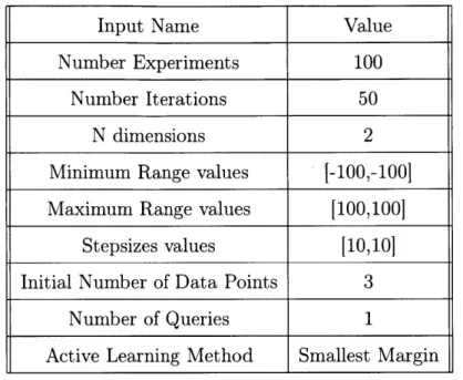
To test the Gaussian Process Classifier and Neural Networks for robustness, we ran Algorithm 3. The inputs that we used for testing the machine learning model robustness are shown in Table 5.3.

Input Name Value

Number Experiments 100

Number Iterations 50

N dimensions 2

Minimum Range values [-100,-1001

Maximum Range values [100,100]

Stepsizes values [10,101

Initial Number of Data Points 3

Number of Queries 1

Active Learning Method Smallest Margin

Table 5.3: ML Model Robustness Test Inputs

The results from our experiments are shown in Table 5.5 and key findings are mentioned in Section 5.4.

Model Area Under the Accuracy Curve Standard Deviation

Neural Networks 47.50 2.60

Gaussian Process Classifier 46.61 1.37

Table 5.4: Results from Model Robustness Tests

Additionally, we provide a boxplot visualization in Figure 5-2 to show how area under the accuracy curve and the variance of the area differ.

50 48 46 44 42 Comparison of GPC vs NN - --401-. 38 GPC NN

Figure 5-2: This graphic depicts the performance of area under the accuracy curve for Gaussian Process Classifiers compared to Neural Networks with one standard deviation bounds.

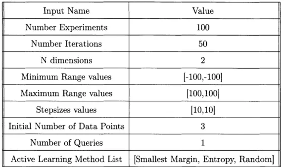
5.4

Active Learning Method Selection

For active learning method selection, we outline the process that we use to simu-late many different variations of active learning experiments for a chosen method in Algorithm 4.