Fast and Accurate Simulation of Multithreaded Sparse Linear Algebra Solvers

HAL Id: hal-01180272

https://hal.inria.fr/hal-01180272v2

Submitted on 26 Jan 2016

HAL is a multi-disciplinary open access

archive for the deposit and dissemination of

sci-entific research documents, whether they are

pub-lished or not. The documents may come from

teaching and research institutions in France or

abroad, or from public or private research centers.

L’archive ouverte pluridisciplinaire HAL, est

destinée au dépôt et à la diffusion de documents

scientifiques de niveau recherche, publiés ou non,

émanant des établissements d’enseignement et de

recherche français ou étrangers, des laboratoires

publics ou privés.

Fast and Accurate Simulation of Multithreaded Sparse

Linear Algebra Solvers

Luka Stanisic, Emmanuel Agullo, Alfredo Buttari, Abdou Guermouche,

Arnaud Legrand, Florent Lopez, Brice Videau

To cite this version:

Luka Stanisic, Emmanuel Agullo, Alfredo Buttari, Abdou Guermouche, Arnaud Legrand, et al.. Fast

and Accurate Simulation of Multithreaded Sparse Linear Algebra Solvers. The 21st IEEE International

Conference on Parallel and Distributed Systems, Dec 2015, Melbourne, Australia. �hal-01180272v2�

Fast and Accurate Simulation of Multithreaded

Sparse Linear Algebra Solvers

Luka Stanisic

, Emmanuel Agullo

, Alfredo Buttari

, Abdou Guermouche

,

Arnaud Legrand

, Florent Lopez

, Brice Videau

∗_{CNRS/Inria/University of Grenoble Alpes, France; firstname.lastname@imag.fr} †_{Inria/University of Bordeaux, France;firstname.lastname@labri.fr} ‡_{CNRS/University Paul Sabatier, Toulouse, France; firstname.lastname@irit.fr}

Abstract—The ever growing complexity and scale of paral-lel architectures imposes to rewrite classical monolithic HPC scientific applications and libraries as their portability and performance optimization only comes at a prohibitive cost. There is thus a recent and general trend in using instead a modular approach where numerical algorithms are written at a high level independently of the hardware architecture as Directed Acyclic Graphs (DAG) of tasks. A task-based runtime system then dynamically schedules the resulting DAG on the different computing resources, automatically taking care of data movement and taking into account the possible speed heterogeneity and variability. Evaluating the performance of such complex and dynamic systems is extremely challenging especially for irregular codes. In this article, we explain how we crafted a faithful simulation, both in terms of performance and memory usage, of the behavior ofqr_mumps, a fully-featured sparse linear algebra library, on multi-core architectures. In our approach, the target high-end machines are calibrated only once to derive sound performance models. These models can then be used at will to quickly predict and study in a reproducible way the performance of such irregular and resource-demanding applications using solely a commodity laptop.

I. INTRODUCTION

To answer the ever increasing degree of parallelism required to process extremely large academic and industrial problems, the High Performance Computing (HPC) community is facing a threefold challenge. First, at large scale, algorithms [1], [2], [3] that used to be studied mostly from a mathematical point of view or for specific problems are becoming more and more popular and practical for applications in many scientific fields. The common property of these algorithms is their very irregular pattern, making their design a strong challenge for the HPC community. Second, the diversity of hardware architectures and their respective complexity make it another challenge to design codes whose performance is portable across architectures. Third, evaluating their performance subsequently also becomes highly challenging.

Until a few years ago, the dominant trend for designing HPC libraries mainly consisted of designing scientific software as a single whole that aims to cope with both the algorithmic and architectural needs. This approach may indeed lead to extremely high performance because the developer has the opportunity to optimize all parts of the code, from the high level design of the algorithm down to low level technical details such as data movements. But such a development

often requires a tremendous effort, and is very difficult to maintain. Achieving portable and scalable performance has become extremely challenging, especially for irregular codes. To address such challenge, a modular approach can be employed. First, numerical algorithms are written at high level, independently of the hardware architecture, as a Directed Acyclic Graph (DAG) of tasks (or kernels) where each vertex represents a computation task and each edge represents a dependency between tasks, possibly involving data transfers. A second layer is in charge of scheduling the DAG, i.e., of deciding when and where to execute each task. In the third layer, a runtime engine takes care of implementing the scheduling decisions, of retrieving the data necessary for the execution of a task (taking care of ensuring data coherency), of triggering its execution and of updating the state of the DAG upon task completion. The fourth layer consists of the tasks code optimized for the target architecture. In most cases, the bottom three layers need not to be written by the application developer since most runtime systems embed off-the-shelf generic scheduling algorithms that efficiently exploit the target architecture.

In this article, we address the third aforementioned chal-lenge related to the performance evaluation of complex algo-rithms implemented over dynamic task-based runtime systems. A previous study [4] has shown that the performance of regular algorithms (such as those occuring in dense linear algebra) on hybrid multi-core machines could be accurately predicted through simulation. We show that it is also possible to conduct faithful simulation of the behavior of an irregular fully-featured library both in terms of performance and memory on multi-core architectures. To this end, we consider the qr_mumps[5] (see SectionIII-Afor more details) sparse direct solver which implements a multifrontal QR factorization (a highly irregular algorithm) on top of the StarPU [6] runtime system and simulate part of the execution with the SimGrid [7] simulation engine (see SectionIII-B).

The rest of the paper is organized as follows. Section II provides some related work on the use of task-based runtime systems in particular in the context of dense and sparse linear algebra solvers. Very few propose a fully integrated simulation mode allowing to predict performance. Then we present in Section IIIand IV the internals ofqr_mumps and how it has been modified to run on top of SimGrid. In Section V, we

explain how we carefully modeled the different components of qr_mumps. Finally we present in Section VI and VII numerous and detailed experimental results that assess how simulation predictions faithfully match with real experiments. We conclude this article in SectionVIIIwith a presentation of current limitations of our work and an opening on envisioned future work.

II. RELATEDWORK

A. Task-based runtime systems and the Sequential Task Flow model

Whereas task-based runtime systems were mainly research tools in the past years, their recent progress makes them now solid candidates for designing advanced scientific software as they provide programming paradigms that allow the program-mer to express concurrency in a simple yet effective way and relieve him from the burden of dealing with low-level architectural details.

The Sequential Task Flow (STF) model simply consists of submitting a sequence of tasks through a non blocking function call that delegates the execution of the task to the runtime system. Upon submission, the runtime system adds the task to the current DAG along with its dependencies which are automatically computed through data dependency analysis [8]. The actual execution of the task is then postponed to the moment when its dependencies are satisfied. This paradigm is also sometimes referred to as superscalar since it mimics the functioning of superscalar processors where instructions are issued sequentially from a single stream but can actually be executed in a different order and, possibly, in parallel depending on their mutual dependencies.

Recently, the runtime system community has delivered more and more reliable and effective task-based runtime systems [6], [9], [10], [11], [12], [13], [14] (a complete review of them is out of the scope of this paper) supporting this paradigm up to the point that the OpenMP board has included similar features in the latest OpenMP standard 4.0 (e.g., the task construct with the recently introduced depend clause). Although this OpenMP feature is already available on some compilers (gcc andgfortran, for instance) we chose to rely on StarPU as it provides a very wide set of features that allows for a better control of the task scheduling policy and because it supports accelerators and distributed memory parallelism which will be addressed in future work.

B. Task-based linear algebra solvers

The dense linear algebra community has strongly adopted such a modular approach over the past few years [9], [15], [16], [17] and delivered production-quality software relying on it. The quality improvement of runtime systems makes it possible to design more irregular algorithms such as sparse direct methods with this approach.

The PaSTIX solver, has been extended [18] to rely on either the StarPU or PaRSEC runtime systems for performing supernodal Cholesky and LU factorizations on multi-core architectures possibly equipped with GPUs. Kim et al. [19]

presented a DAG-based approach for sparse LDLT

factor-izations where OpenMP tasks are used and dependencies between nodes of the elimination tree are implicitly handled through a recursive submission of tasks, whereas intra-node dependencies are essentially handled manually. The baseline code used in this article is a QR multifrontal solver running on top the StarPU runtime system [5].

Interestingly, to better extract potential parallelism, these solvers (e.g., PaSTIX [18] andqr_mumps [20]) were already often designed with, to some extent, the concept of task before having in mind the goal of being executed on top of a runtime system. It is also the case of the SuperLU [21] supernodal solver. This design offered the opportunity to produce an advanced mechanism for simulating its performance [22]. The present work however differs from [22] mostly by the fact that the execution of qr_mumps is dynamic and deeply non-deterministic, which greatly complicates its performance evaluation.

III. PRESENTATION OFSIMGRID/STARPU/qr_mumps A. qr_mumps

The multifrontal method, introduced by Duff and Reid [23] as a method for the factorization of sparse, symmetric linear systems, can be adapted to the QR factorization of a sparse matrix thanks to the fact that the R factor of a matrix A and the Cholesky factor of the normal equation matrix ATA share the same structure under the hypothesis that the matrix A is Strong Hall. As in the Cholesky case, the multifrontal QR factorization is based on the concept of elimination tree introduced by Schreiber [24] expressing the dependencies between elimination of unknowns. Each vertex f of the tree is associated with kf unknowns of A. The coefficients of

the corresponding kf columns and all the other coefficients

affected by their elimination are assembled together into a relatively small dense matrix, called frontal matrix or, simply, front, associated with the tree node (see Figure 2). An edge of the tree represents a dependency between such fronts. The elimination tree is thus a topological order for the elimination of the unknowns; a front can only be eliminated after its children. We refer to [20], [25], [26] for further details on high performance implementation of multifrontal QR methods.

The multifrontal QR factorization then consists in a tree traversal following a topological order (see line 1 in Figure1 (left)) for eliminating the fronts. First, the activation (line 3) allocates and initializes the front data structure. The front can then be assembled (lines 5-12) by stacking the matrix rows associated with the kfunknowns with uneliminated rows

resulting from the processing of child nodes. Once assembled, the kf unknowns are eliminated through a complete QR

factorization of the front (lines 14-21); for these last two operations we assume that a 1D, block-column, partitioning is applied to the fronts. This produces kf rows of the global

R factor, a number of Householder reflectors that implicitly represent the global Q factor and a contribution block formed by the remaining rows. These rows will be assembled into the

Sequential version

1 forall fronts f intopological order

! allocate and initialize front

3 callactivate(f) 5 forallchildren c of f

forallblockcolumns j=1...ninc 7 ! assemble column j of c into f

callassemble(c(j), f) 9 end do ! Deactivate child 11 calldeactivate(c) end do 13 forallpanels p=1...n inf 15 ! panel reduction of column p

callpanel(f(p))

17 forallblockcolumns u=p+1...n inf

! update of column u with panel p

19 callupdate(f(p), f(u))

end do

21 end do end do

23

STF version

forallfronts f intopological order

! allocate and initialize front

callsubmit(activate, f:RW, children(f):R)

forallchildren c of f

forall blockcolumns j=1...ninc

! assemble column j of c into f

callsubmit(assemble, c(j):R, f:RW)

end do

! Deactivate child

callsubmit(deactivate, c:RW)

end do

forallpanels p=1...n inf

! panel reduction of column p

callsubmit(panel, f(p):RW)

forall blockcolumns u=p+1...nin f

! update of column u with panel p

callsubmit(update, f(p):R, f(u):RW)

end do end do end do

callwait_tasks_completion()

Figure 1. Sequential version (left) and corresponding STF version from [5] (right) of the multifrontal QR factorization with 1D partitioning of frontal matrices.

Figure 2. Typical elimination tree: each node corresponds to a front and the resulting tree is traversed from the bottom to the top. To reduce the overhead incurred by managing a large number of fronts, subtrees are pruned and aggregated into optimized sequential tasks (Do_subtree) depicted in gray. Activate Assemble Panel Update Deactivate

Figure 3. The STF code allows to express the complex dependencies induced by the staircase. The resulting DAG is dynamically scheduled by the runtime system.

parent front together with the contribution blocks from all the sibling fronts.

The multifrontal method provides two distinct sources of concurrency: tree and node parallelism. The first one stems from the fact that fronts in separate branches are independent and can thus be processed concurrently; the second one from the fact that, if a front is large enough, multiple threads can be used to assemble and factorize it. Modern implementations exploit both sources of concurrency which makes schedul-ing difficult to predict, especially when relyschedul-ing on dynamic scheduling which is necessary to fully exploit the parallelism delivered by such an irregular application.

One distinctive feature of the multifrontal QR factorization is that frontal matrices are not entirely full but, prior to their factorization, can be permuted into a staircase structure that allows for moving many zero coefficients in the bottom-left corner of the front and for ignoring them in the subsequent computation. Although this allows for a considerable saving in the number of operations, it makes the workload extremely irregular and the cost of kernels extremely hard to predict even in the case where a regular partitioning is applied to fronts, which makes it challenging to model.

Figure1(right) shows the STF version from [5] (used in the present study) of the multifrontal QR factorization described above. Instead of making direct function calls (activate, assemble, deactivate, panel, update), the equivalent STF code submits the corresponding tasks (see Figure 3). Since the data onto which these functions operate as well as their access mode (Read, Write or Read/Write) are also specified, the runtime system can perform the superscalar analysis while the submission of task is progressing. For instance, because an assemble task accesses a block-column f(i) before a panel task accesses the same block-column in Write mode, a dependency between those two tasks is inferred. Figure 3

shows (on the right side) the resulting DAG associated with a small, artificial, elimination tree (on the left side). It must be noted that in real life problems the elimination tree commonly contains thousands of nodes and the associated DAG hundreds of thousands of tasks.

Because the number of fronts in the elimination tree is commonly much larger than the number of resources, the partitioning is not applied to all of them. A logical tree pruning technique [20] is used similar to what proposed by Geist and Ng [27]. Through this technique, a layer in the elimination tree is identified such that each subtree rooted at this layer is treated in a single task with a purely sequential code. This new type of tasks, which are nameddo_subtree, is represented in Figure2 as the gray layer.

B. StarPU/SimGrid

In [4], we explained how we crafted a coarse-grain hy-brid simulation/emulation of StarPU [6], a dynamic runtime system for heterogeneous multi-core architectures, on top of SimGrid [7], a simulation toolkit initially designed for distributed system simulation. In our approach, among the four software layers mentioned in Section~III-B(high-level DAG description, scheduling, runtime and kernels), the first three ones are emulated in the SimGrid framework. Their actual code is indeed executed except that a few primitives (such a thread synchronizations) are handled by SimGrid. In the fourth layer, the task execution is simulated. An initial calibration of the target machine is run once to derive performance profiles and models (interconnect topology, data transfers, computation kernels) that are given as an input to SimGrid. Subsequent simulations can then be performed in a reproducible way on personal commodity laptops without requiring any further access to the target machines. We showed in [4] how this approach enables to obtain accurate performance prediction of

two dense linear algebra applications on a wide variety of hy-brid (comprising several CPUs and GPUs) architectures. Our extensive study demonstrated that non-trivial scheduling and load balancing properties can be faithfully studied with such approach. It has also been used to study subtle performance issues that would be quite difficult and costly to evaluate using solely real experiments [28].

IV. CHALLENGES FOR PORTING qr_mumps ON TOP OF SIMGRID

The extension of this methodology to an highly irregular algorithm such as the multifrontal QR method is not immediate because the fourth layer (kernel execution) is much harder to simulate. When working with dense matrices, it is common to use a global fixed block size and a given kernel type (e.g., dgemm) is therefore always called with the same parameters throughout the execution, which makes its duration on the same processing unit very stable and easy to model. On the contrary, in the qr_mumps factorization, the amount of work that has to be done by a given kernel greatly depends on its input parameters. Furthermore, these parameters may or may not be explicitly given to the StarPU runtime in the original qr_mumpscode.

The challenges for designing a reliable simulation of qr_mumps thus consists in identifying which parameters sig-nificantly impact the task durations and propagating these information to SimGrid. Some parts of the StarPU code responsible for interacting with SimGrid were also modified to detect specific parametric kernels and predict durations based on the captured parameter values. We have also extended the StarPU tracing mechanism so that such kernel parameters are traced as well, which is indispensable to obtain traces that can be both analyzed and compared between real and simulated executions.

V. MODELING qr_mumpsKERNELS

We conducted an in-depth analysis of the temporal behavior of the different kernels invoked in qr_mumps. We discovered and assessed that Panel andUpdate have a similar structure and that the only parameters that influence their duration can be obtained from the corresponding task parameters and there-fore determined by inspecting the matrix structure, without even doing the factorization for real. This eases the modeling of such kernels since such information can be used to define the region in which such parameters evolve and to design an informed experiment design to characterize the performance of the machine.

The other three kernels (Do_subtree,Activateand Assem-ble) show different behavior and the explaining parameters were more difficult to identify. In the following we describe our modeling choices for each kernel, detailing how and why particular parameters proved to be crucial.

A. Simple Negligible Kernels

As illustrated by Figure 8 (top-right histogram), the De-activate kernel has a very simple duration distribution. We

remind that this kernel is responsible solely for deallocating the memory at the end of the matrix block factorization. It is thus not surprising that these tasks are very short (a few milliseconds) and are negligible compared to the other kernels. Furthermore, there are only a few instances of such tasks even for large matrices and the cumulative duration of the Deactivate kernels is thus generally less than 1% of the overall application duration (makespan). Therefore, we decided to simply ignore this kernel in the simulation, injecting zero delay whenever it occurs. So far, this simplification has not endangered the accuracy of our simulation tool.

B. Parameter Dependent Kernels

Certain qr_mumps kernels (Panel and Update) are mostly wrappers of LAPACK/BLAS routines in which the vast major-ity of the total execution time is spent. Their duration depends essentially on their input arguments, which define the geom-etry of the submatrix on which the routines work. Although these routines execute very different kind of operations, they can be modeled in a similar way.

1) Panel: The duration of Panel kernel mostly depends on the geometry of the data block it operates upon, i.e., on MB (height of the block), NB (width of the block) and BK (number of rows that should be skipped). This kernel simply encapsulates the standard dgeqrt LAPACK subroutine that performs the QR factorization of a dense matrix of size m × n with m = MB − (BK − 1) × NB and n = NB . Therefore, its a prioricomplexity is:

TPanel= a + 2b(NB2× MB ) − 2c(NB3× BK ) + 4d

3 NB

3_,

where a, b, c and d are machine and memory hierarchy dependent constant coefficients.

Table I

LINEARREGRESSION OFPanel

PanelDuration N B3 _{1.50 × 10}−5 _{(1.30 × 10}−5_{, 1.70 × 10}−5₎ ∗∗∗ N B2_{∗ M B 5.49 × 10}−7 _{(5.46 × 10}−7_{, 5.51 × 10}−7₎ ∗∗∗ N B3_{∗ BK −5.52 × 10}−7_{(−5.57 × 10}−7_{, −5.48 × 10}−7₎ ∗∗∗ Constant −2.49 × 101_{(−2.83 × 10}1_{, −2.14 × 10}1₎ ∗∗∗ Observations 493 R2 _0.999 Note: ∗p<0.1;∗∗p<0.05;∗∗∗p<0.01

Such linear combination of parameter products fits the linear modeling framework and the summary of the corresponding linear regression is given in Table I. For each parameter combination in the first column (NB3, NB2 × MB , and NB3×BK ), we provide an estimation of the corresponding co-efficient along with the 95% confidence interval. These values correspond to the a, 2b, 2c and 4d₃ from the previous formula. The standard errors are always at least one order of magnitude lower than the corresponding estimated values, which means that the coefficient estimates is accurate. Furthermore, the three stars for each parameter in the last column indicate that

the estimates of the coefficients are all significantly different from 0, which means that these parameters are significant. This hints that the model is minimal and that we can not simplify it further by removing parameters without damaging its precision. Finally, the most important indicator is the adjusted R2 value1_{, which in our case is almost 1, which}

indicates that this model has a very good predictive power. We also checked the linear model hypothesis (linearity, homoscedasticity, normality) by analyzing the corresponding standard plots provided by the statistical language R. Only the normality assumption did not hold perfectly in our case, which is known to not harm the quality of the regression.

2) Update: The duration of theUpdatekernel also depends on the geometry of the data it operates upon, defined by the same MB , NB , and BK parameters. This kernels simply wraps the LAPACK dgemqrt routine which applies k Householder reflections of size m, m − 1, ..., m − k + 1 on a matrix of size m × n where m, n and k are equal to M B − (BK − 1) × N B, N B and N B, respectively. Therefore, its a priori complexity is defined as:

TUpdate= a0+ 4b0(NB

2

× MB ) − 4c0(NB3× BK ) + 3d0NB3 Table II

LINEARREGRESSION OFUpdate

UpdateDuration N B3 _{1.59 × 10}−9_{(−6.93 × 10}−8_{, 7.25 × 10}−8₎ N B2_{∗ M B 4.37 × 10}−7_{(4.36 × 10}−7_{, 4.37 × 10}−7₎ ∗∗∗ N B3_{∗ BK −4.37 × 10}−7_{(−4.38 × 10}−7_{, −4.36 × 10}−7₎ ∗∗∗ Constant 8.33 × 10−1(7.12 × 10−1, 9.54 × 10−1) ∗∗∗ Observations 20,893 R2 _0.998 Note: ∗p<0.1;∗∗p<0.05;∗∗∗p<0.01

The same approach can thus be used and the R regression summary is provided in Table II. The coefficient estimates are obviously different from the ones of the Panel kernel since the nature of the two kernels is different. The most notable difference is certainly the N B3 coefficient whose influence cannot be accurately estimated and may thus appear as insignificant. However, this can be explained by the fact that for this particular matrix, the parameter range of BK is limited, which leads to a confounding of the effects of NB3 with the ones of NB3× BK .

It is also interesting to note that this model is based on a much larger set of observations, which is expected since one Panel is followed by many Updates. Finally, the R2 value reported in TableIIis again very close to 1, which shows the excellent predictive power of this simple model.

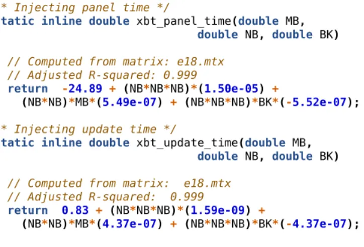
3) Simulation: From the previous R linear regressions (tables I and II), we automatically generate C code for the 1_{The coefficient of determination, denoted R}2_{, indicates how well data fit} a statistical model and ranges from 0 to 1. An R2 of 0 indicates that the model explains none of the variability of the response data around its mean while an R2 of 1 indicates that the regression line perfectly fits the data.

/* Injecting panel time */

static inline double xbt_panel_time(double MB, double NB, double BK) {

// Computed from matrix: e18.mtx // Adjusted R-squared: 0.999

return -24.89 + (NB*NB*NB)*(1.50e-05) +

(NB*NB)*MB*(5.49e-07) + (NB*NB*NB)*BK*(-5.52e-07); }

/* Injecting update time */

static inline double xbt_update_time(double MB, double NB, double BK) {

// Computed from matrix: e18.mtx // Adjusted R-squared: 0.999

return 0.83 + (NB*NB*NB)*(1.59e-09) +

(NB*NB)*MB*(4.37e-07) + (NB*NB*NB)*BK*(-4.37e-07); }

Figure 4. Automatically generated code for computing the duration ofPanel

andUpdatekernels.

simulation of these kernels (see Figure 4) and link it to SimGrid. When simulating qr_mumps, whenever Panel or Update is called, their parameters are given as an input to these functions. The calling thread is then blocked during the corresponding duration estimation, thereby increasing the simulation time without actually executing the tasks.

It is important to understand that these two kernels are the most critical ones regarding overall simulation accuracy and that the precision of their estimation greatly influences both the makespan and the dynamic scheduling.

C. Matrix Dependent Kernels

Modeling kernels based on their signature is quite natural but it is unfortunately not applicable to all kernels. Some of them are more than simple calls to regular LAPACK/BLAS subroutines. These tasks execute a sequence of operations that depends on the matrix structure as well as on the organization of the previously executed tasks. Therefore, such kernels cannot be modeled simply from their input parameters. The actual amount of work performed by the task can however be estimated by taking into account the size of the submatrix and its internal structure. Such complexity is required as large parts of the matrix blocks are filled with zeros. These regions are thus skipped by kernel operations. Three kernels therefore require a specific expertise on the multifrontal QR method and theqr_mumpscode to provide such workload estimates.

• Do_subtree: Both an estimation of the number of floating point operations it needs to perform and the number of nodes it has to manage are required to model the duration of this kernel.

• Activate: The duration of this kernel is mainly governed by two factors: the number of coefficients that have to be set to zero and the number of non-zero coefficients it has to assemble from children nodes.

• Assemble: The complexity of this kernel is directly linked to the total number of non-zero coefficients that needs to be copied to the parent node. However such memory

intensive operation is more subject to variability than the other computing kernels.

Analyzing the execution of these kernels and constructing models can then be performed as in SubsectionV-Busing the R language and simple linear regressions. TableIIIpresents a summary of the prediction quality for each kernel as well as the minimal number of parameters that have to be taken into account. For all of them, the adjusted R2is close to 1, which indicates an excellent predictive power.

Table III

SUMMARY OF THE MODELING OF EACH KERNEL BASED ON THE E18

MATRIX ON FOURMI(SEESECTIONVIFOR MORE DETAILS).

Panel Update Do_subtree Activate Assemble

1. NB NB #Flops #Zeros #Coeff

2. MB MB #Nodes #Assemble /

3. BK BK / / /

R2 _{0.99 0.99 0.99 0.99 0.86}

VI. EXPERIMENTALMETHODOLOGY

To evaluate the quality of our approach, we used two different kind of nodes from the Plafrim2platform. The fourmi nodes comprise 2 Quad-core Nehalem Intel Xeon X5550 with a frequency of 2,66 GHz and 24 GB of RAM memory and the riri nodes comprise 4 Deca-core Intel Xeon E7-4870 with a frequency of 2,40 GHz and 1 TB of RAM memory. The fourmi nodes proved to be easier to model as their CPU architecture is well balanced with 4 cores sharing L3 cache on each of the 2 NUMA nodes. Such configuration leads to little cache contention. However, the RAM of these nodes is limited and thereby limits the matrices that can be factorized to a certain size. Although the huge memory of the riri machine puts almost no restriction on the matrix choice, its memory hierarchy with 10 cores sharing the same L3 cache lead to cache contention that can be tricky to model.

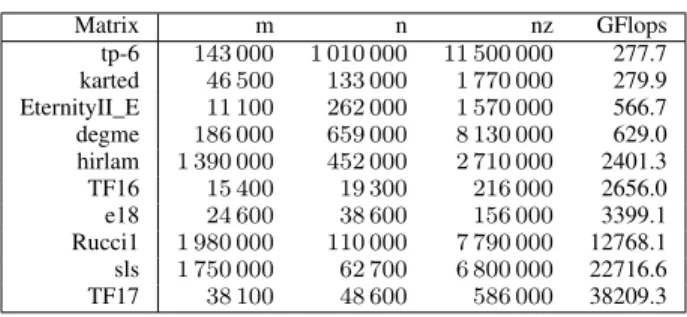
The matrices we used for evaluating our approach are presented in the TableIVand come from the UF Sparse Matrix Collection3 _{plus one from the HIRLAM}4 _{research program.}

Table IV

MATRICES USED FOR THE EXPERIMENTS

Matrix m n nz GFlops tp-6 143 000 1 010 000 11 500 000 277.7 karted 46 500 133 000 1 770 000 279.9 EternityII_E 11 100 262 000 1 570 000 566.7 degme 186 000 659 000 8 130 000 629.0 hirlam 1 390 000 452 000 2 710 000 2401.3 TF16 15 400 19 300 216 000 2656.0 e18 24 600 38 600 156 000 3399.1 Rucci1 1 980 000 110 000 7 790 000 12768.1 sls 1 750 000 62 700 6 800 000 22716.6 TF17 38 100 48 600 586 000 38209.3

The execution time of a single kernel on a certain machine greatly depends on the machine characteristics (namely CPU

2_{https://plafrim.bordeaux.inria.fr/}

3_{http://www.cise.ufl.edu/research/sparse/matrices/} 4_{http://hirlam.org/}

frequency, memory hierarchy, compiler optimization, etc.). Obtaining accurate timing is thus a critical step of the model-ing. To predict the performance of the factorization of a set of matrices on a given experimental platform, we first benchmark the kernels identified in the previous section.

For the kernels that have clear dependency on the matrix geometry (Panel and Update), we wrote simple sequential benchmarking scripts, that pseudo-randomly choose different parameter values, allocate the corresponding matrix and finally run the kernel, capturing its execution time. However, for kernels (Do_subtree,ActivateandAssemble) whose code is much more complex and depends on many factors, including even dependencies on previously executed tasks, creating a simplistic artificial program that would mimic such a sophis-ticated code is very difficult. Since each sparse matrix has a unique structure, the corresponding DAG is very different and the kernel parameters (such as height and width) greatly vary from one matrix factorization to another. For example, the qr_mumps factorization of cat_ears_4_4 executes a very large number of "small" Do_subtree kernels (each with a small amount of work), while some others matrices, such as e18, have much fewer instances of this kernel, but with a bigger workload. Consequently, it is very hard to construct a single linear model that is appropriate for both use cases. The inaccuracies caused by such model imperfection can produce either underestimation or overestimation of the kernel duration and thus of the whole application makespan as well. Therefore, to benchmark such kernels we rely on traces generated by a real qr_mumps execution (possibly on different matrices than the ones that need to be studied) instead of a careful experiment design.

The result of this benchmark is analyzed with R to obtain linear models that are then provided to the simulation. At each step of the regression, we control that the models are adequate through a careful inspection of the regression summaries and of the residual plots. These models are then linked with the simulator and the experimental platform is then of no longer use as qr_mumps can then be run in simulation mode on a commodity laptop. Using a recent and more powerful machine only improves the simulation speed and possibly allows for running several simulations in parallel.

To evaluate the validity of our approach, we need to compare real execution outcomes (denoted by Native in the sequel) with simulations outcomes (denoted by SimGrid in the sequel). Therefore, we execute qr_mumpsfor the different matrices and collect not only the execution time but also an execution trace with information for each kernel as well as when memory is allocated and deallocated. When running on simulation, due to the structure of our integration, we can collect a trace of the same nature and thus compare the real execution to the simulation in details.

To summarize, our experimentation workflow can be de-scribed in the following four steps:

1) Run once a designed calibration campaign on the target machine that spans the desired parameter space corre-sponding to the different matrices.

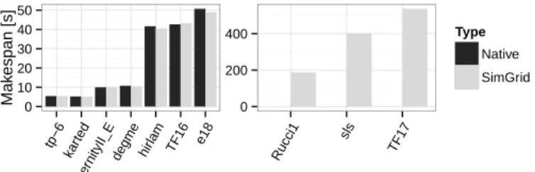
0 10 20 30 40 50 0 200 400 tp−6 kar ted Eter

nityII_E degmehir

lam TF16 e18 Rucci1 sls TF17 Mak espan [s] Type Native SimGrid

Figure 5. Makespans on the 8 CPU cores fourmi machine.

2) Analyze benchmarking outputs and execution traces, fit-ting the observations into linear models for each kernel. Add such models to SimGrid.

3) Run simulations on a commodity machine.

4) Validate simulation accuracy by comparing makespans, traces and memory consumption with the Native execu-tion.

Following the principles and the Git/Org-mode workflow presented in [29], all the results that are given in this docu-ment are also available online5 for further inspection. This repository additionally contains source code of qr_mumps, StarPU and SimGrid along with all the scripts for running the experiments, the calibrations and conducting the analysis, making our work as reproducible as possible. Supplementary data (e.g., produced by "unsuccessful" experiments and that can be very informative to the reader) can also be found at the same location.

VII. SIMULATIONQUALITYEVALUATION A. Makespan and Execution Evaluation

1) Evaluation on the fourmi machine: Figure5 depicts the overall execution time of qr_mumps when factorizing the dif-ferent matrices of TableIV. The SimGrid predictions are very accurate, as they are never larger than 3%. It should be noted that our predictions are systematically slight underestimations of the actual execution time as our coarse grain approach ignores the runtime overhead and a few cache effects.

Still, focusing solely on a single number at the end of the execution hides all the details about the operations performed during the execution. Therefore, we also investigated the whole scheduling in details, comparing Native to SimGrid execution traces. An example of such investigation for the e18 matrix (it is the one exhibiting the largest difference between Native and SimGrid makespans) is shown in Figure6. To make the Gantt charts as readable as possible, we retain only the modeled kernels and idle state, filtering overlapping states related to the runtime control.

qr_mumps starts by executing many Do_subtree kernels and executes all the remaining ones soon after. Most of the time is spent running Update while the Panel is executed regularly. Towards the end, there are fewer and fewer tasks with more and more dependencies between them, and many

5_{http://starpu-simgrid.gforge.inria.fr/. We also provide on github an}

exam-ple of an easy to accesspretty-printed report on a traceas well as information

onhow the trace was captured.

cores have thus to remain idle. The Native and SimGrid traces are extremely close. A noticeable difference can be seen at the very beginning as in simulation all workers start exactly at time 0, they all pick Do_subtree tasks that are the leaves of the DAG and thus the first ready tasks. Although the real execution tends to run in the same manner, it is not so strict and several workers pick Activate tasks available right after the first Do_subtree terminates. Another small discrepancy between the two traces can be noticed at the end of the execution where the idle time is distributed in a quite different way. This is however related to the difference of scheduling decisions taken by the runtime. Indeed, we remind that the StarPU runtime schedules tasks dynamically and thus even two consecutive Native executions can lead to quite different execution structures even if their total duration is generally similar. Idle time distributions similar to the one of the SimGrid trace can also be observed in real executions. However, gantt charts of such densely packed traces of dynamic schedules can sometimes be misleading. The first issue comes from the fact that there is a huge number of very small states that have to be aggregated during the graphical representation which is limited by the screen or printer resolution. Many valuable information can be lost in such process and the result may be biased [30]. Second, it is very hard to quantify the resemblance of the two traces that are dynamically scheduled, as even when the task graph is fixed, the tasks will naturally have very different starting times from an execution to another. Therefore, we compared different and more controlled aggregates.

For example, Figure 8 compares the distributions of the duration of each kernel for a real execution and a simulation (we use the same two traces of the e18 matrix that were used earlier). The upper row presents kernel distributions from the Native trace, while in the bottom row are the ones predicted by the SimGrid simulation. The modeling technique described in Section V proves very satisfactory, since distributions match quite accurately. The only kernel for which we can observe a slightly larger discrepancy isAssemble, which was indeed very hard to model and had the worst R2 value. However, in prac-tice this kernel is rarely on the critical path of the qr_mumps execution and is often covered by other kernels. Additionally, the overall duration of all Assembletasks is relatively small compared to others and thus such inaccuracies of the model do not greatly affect the final simulation prediction.

Studying distribution applies a temporal aggregation and discards any notion of time and when a specific task was executed. This can hide interesting facts about certain events or a particular group of tasks that occurred in a distinct period of time during the whole application run. Figure7 tracks the execution of thePanelkernel and indicates the duration of the tasks at each time. To ease the correspondence between the real execution and the simulation, the color of each point is related to the job id of the task. Both colors and the pattern of the points suggest that the traces match quite well. Even though the scheduling is not exactly the same, it is still very close. Similar analysis have been performed for all the other

Figure 6. Gantt chart comparison on the 8 CPU cores fourmi machine. ● ● ● ● ● ● ● ● ● ● ● ● ● ● ● ● ● ● ●● ● ● ● ● ● ● ● ● ● ●●●●●●●●●●●●●●●●●●●●●●●●● ●●●●●●●●●●● ● ● ● ● ● ● ● ● ● ● ● ● ● ● ● ● ● ● ● ●●●●●●●●●●●●●●● ● ● ● ●●●●●●●●● ● ● ● ● ● ● ● ●●●●●●●●●●●●●●●●●●●●●●●●●●●●● ● ● ● ●●●●●●●●●●●●●●●●●●●●●●●●●●●●●●●●●● ● ● ● ● ● ● ● ●●●●●●●●●● ● ● ●●●●●●●●●●●●●●●●● ●●●●●●●●●●●●●●●●●●●●●●●●●●●●●●●●●●●●●●●●●●●●●●●●●●●●●●●●●●●●●●●●●●●●●●●●●●●●●●● ●●●●●●●●●●●●●●●●●● ● ● ● ● ● ● ●●●● ● ●●●●●●● ●●●●● ●●●●●● ●●●●●●●●●●●●●●●●_●●●●●●●●●●●●●●●●●●●●●●●●●●●●●●●●●●●●●●●●●●●●●●●●●●●●●●●●●●●●●●●● ● ● ●●●●●●●●●●●●●●●●●● ●●●●●●● ●●●●●●● ●●●●●●●●●●●●●●●●●●●●●●● ● ●●●●●●●● ● ● ● ● ● ● ● ● ● ● ● ● ● ● ● ● ● ● ● ●● ●●●●● ●●●●●●●●●●●●●●●●●●●●●●●●●●●●●●●●●●●●●●●● ●●●●●●●●●●●●●●●●●●●●●●●●●●●●●●●●●●●●●●●●●●●●●●●●●●●●●●●●●●●●●●●●●●●●●●●●●●●●●●●●●● ● ● ● ●●●●●●●●●●●●●●●●●●●●●●●●●●●●●●●●●● ● ● ● ● ● ● ● ● ● ● ● ●● ● ● ● ● ● ● ● ● ●●●●●●●●●●●●●●●●●●●●●●●●●●●●●●●● ●●●●●● ●●●●●●●●●●●●●●●●●●● ●●●●●●●●●●●●●●●●●●●●●●●●●● ●●●●●●●●●●●●●●●●●●●●●●●●●●●●●●● ●●●●●●●●●●●●●●●●●● ●●●●●●● ● ● ●●●●●●●●●●●●●●●●●●●●●●●●●●●●●●●●●●●●●●●●●●●●●●●●●●●●●●●●●●●●●●●●●●●●●●●●●●●●●●●● ● ●●●●●●●●●●● ●●●●●●●●●●●●●●●●●●●●●●●●●●●●●●●●●●● ●●●●●●●●●●●●●●●●●●●_● Native, Panel SimGrid, Panel 0 25 50 75 0 25 50 75 0 10,000 20,000 30,000 40,000 50,000 Time [ms] K er nel Dur ation [ms]

Figure 7. ComparingPanelas a time sequence on the 8 CPU cores fourmi machine. Color is related to the task id.

Native, Do_subtree SimGrid, Do_subtree 0 3 6 9 0 3 6 9 0 50 100 Number of Occur ances Native, Activate SimGrid, Activate 0 5 10 15 20 0 5 10 15 20 0 250 500 750 Native, Panel SimGrid, Panel 0 100 200 0 100 200 0 25 50 75 Native, Update SimGrid, Update 0 2000 4000 6000 0 2000 4000 6000 0 20 40 60 Native, Assemble SimGrid, Assemble 0 100 200 300 0 100 200 300 0 10 20 30 Native, Deactivate SimGrid, Deactivate 0 10 20 30 0 10 20 30 0 25 50 75 Kernel Do_subtree Activate Panel Update Assemble Deactivate

Figure 8. Comparing kernel distribution duration on 8 CPU cores fourmi machine.

10 Cores, Small matrices 10 Cores, Large Matrices

40 Cores, Small matrices 40 Cores, Large Matrices 0 10 20 30 40 0 100 200 300 400 500 0 5 10 15 20 0 50 100 150 200 tp−6 kar ted Eter

nityII_E degmehir

lam TF16 e18 Rucci1 sls TF17 tp−6 kar ted Eter

nityII_E degmehir

lam TF16 e18 Rucci1 sls TF17 Mak espan [s] Type Native SimGrid

Figure 9. Results on the riri machine using 10 or 40 CPU cores. When using a single node (10 cores), the results match relatively well although not as well as for the fourmi machine due to a more complex and packed processor architecture. When using 4 nodes (40 cores), the results are still within a reasonnable bound despite the NUMA effects.

kernels as well and the results were very much alike. 2) Evaluation on the riri machine: To validate our ap-proach, we have experimented on a different architecture. The results presented in Figure 9 show a more important error of the SimGrid predictions, that is now averaging 8.5%. Such inaccuracy mostly comes from the fact that riri has a specific architecture, where the 10 cores used for the experiments all share the same L3 cache. The pressure on the cache produced by all the workers executing kernels in parallel decreases the

overall performance, which is not correctly captured by our models. Still, the SimGrid predictions stay reasonably close to the Native ones and thus very useful to users and developers. One step further in our experimental campaign was to compare executions on the full machine, using all 40 cores. As expected, the largest prediction error doubled (Figure 9), but the results can still be considered as good since all the tendencies are well captured. In particular, non trivial results can be obtained such as the fact that the TF17 matrix benefits much more from using several nodes than the sls matrix. B. Memory Consumption

Working on several parts of the elimination tree in parallel provides more scheduling opportunities, which improves pro-cessor occupancy. But it also increases memory requirements, which can have a very negative influence on performance. The most critical criteria regarding memory is the peak memory consumption of the application. A single wrong scheduling decision can dramatically increase it and potentially result in memory swapping between the RAM and the disk.

Since the amount of work that can be executed in parallel is generally limited and very matrix dependent, finding the right trade-off between memory consumption and the efficient use of the whole set of available cores is crucial for obtaining the best performance [31]. To evaluate a new factorization algorithm or a different scheduling strategy, one thus has to perform a large number of costly experiments on various matrices. Using simulation can greatly reduce the cost of such study as it does not require the access to the actual experimental machines, often shared between many users. It

Native 1 SimGrid Native 2 Native 3 0 1 2 3 0 1 2 3 0 1 2 3 0 1 2 3 0 10,000 20,000 30,000 40,000 Time [ms] Allocated Memor y [GiB]

Figure 10. Memory consumption evolution. The blue and red parts corre-spond to theDo_subtreeandActivatecontribution.

can be performed much faster and several simulations with different parameters can even be run in parallel. In our solution no actual memory is neither allocated nor deallocated for the data, as the corresponding malloc calls are only simulated by SimGrid. However, the size for the required array allocation and deallocation is still traced. This allows for reconstructing memory usage, providing the memory peak prediction of the simulation. Since SimGrid faithfully represents the runtime execution (as it was presented in the previous subsections), its execution will go through the DAG in a very similar way to the Native run. Therefore, the memory peak predicted by SimGrid will be very close to the one observed in Native experiments. Beyond the memory peak, it is also interesting to study the evolution of memory consumption throughout the execution. Figure10shows the evolution of the total amount of memory allocated byqr_mumpswhen factorizing the hirlam matrix for three Native executions and for a simulation. The three Native executions correspond to three consecutive runs performed with exactly the same source code and environment. Such analysis allows for identifying where the scheduling was not optimal and what parts of the application should be improved to increase the overall performance. Although the memory consumption evolution is very similar between different exper-iments it is far from being identical since runtime scheduling decisions are made dynamically. The evolution predicted by SimGrid is remarkably difficult to distinguish from the three other ones, which shows that our approach allows for faithfully predicting memory consumption.

C. Extrapolation

When sufficient care is taken on benchmarking and kernel profiling, we believe that our approach allows for performing faithful performance prediction of the execution on large computer platforms. Based on models obtained from a single CPU calibration, we can extrapolate the simulation on a larger numbers of cores. These simulation results are certainly not as accurate as the ones presented in Section VII, but can still show general trends. New phenomena that haven’t been observed yet may occur at large scale but the simulation somehow allows for obtaining an "optimistic" performance prediction that will be achieved "if nothing goes wrong".

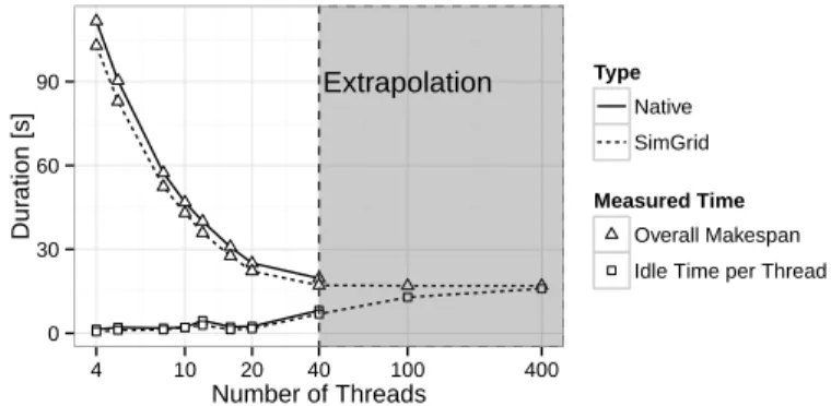
Extrapolation 0 30 60 90 4 10 20 40 100 400 Number of Threads Dur ation [s] Type Native SimGrid Measured Time Overall Makespan Idle Time per Thread

Figure 11. Extrapolating results for e18 matrix on 100 and 400 CPU cores.

Researchers can thus observe how their matrix factorization would perform in an ideal context. Since certain parts tend to be underestimated (e.g., contention) in the simulations, Sim-Grid results provide theoretical performance bounds, above which application could not pass on the target machine.

Figure11shows the performance obtained when factorizing the e18 matrix with different numbers of cores. Together with the overall makespan, we indicate how much time in average each core spends idle. With a small number of workers, each thread has enough work as qr_mumps is well parallelized. However, the execution is limited by the critical path in the DAG of tasks and thus above a given platform size, most of the cores remain idle, waiting for task dependencies to be satisfied. Increasing the number of threads beyond this point does not improve the overall performance, but only decreases the efficiency of the workers. After comparing our simulation results to the Native execution for up to 40 cores on the riri machine, we decided to use the same kernel models and investigate what performance could be expected from a larger machine comprising the same kind of nodes. The simulation results actually predict that the makespan will not improve any further and that most cores will be idle. Investigating more in detail the trace simulated for 100 cores would allow to know whether the critical path is hit or if further improvements can still be expected with a better scheduling.

VIII. CONCLUSION

This article extends our previous work [4] that addressed the simulation of dynamic dense linear algebra solvers on hybrid machines, by considering a sparse multifrontal linear algebra solver. Modeling the irregular internals of such ap-plication is much more challenging and required a careful study. We show through extensive experimental results that we manage to accurately predict both the performance and the memory usage of such applications. Our proposal also allows for quickly simulating such dynamic applications using only commodity hardware instead of expensive high-end machines. As an illustration, factorizing the TF17 matrix on a 40 core machine (see Section VI) requires 157s and 58GiB of RAM while simulating on a laptop its execution only takes 57s and 1.5GiB of RAM. Being able to quickly obtain performance and details of memory consumption of such applications on a

commodity laptop is a very useful feature to the qr_mumps users and developers, as they can easily test the influence of various scheduling, parameters or even code modifications. The SimGrid simulation mode is thus integrated in the latest versions of StarPU and of qr_mumps.

The current main limitation of our work concern the faithful modeling of very large NUMA machines were data transfers are implicit and where performance degradation of computation kernels due to cache sharing can be significant. We think such issues can be addressed through a careful model calibration taking into account potential interferences and through the use of explicit data transfers. This could be done through the use of StarPU-MPI [32] that was designed exploit large distributed machines. The simulation of StarPU-MPI based applications with SimGrid is underway as well as the exploitation of hybrid machines (comprising GPUs) in qr_mumps. These developments will allow us to investigate per-formance evaluation of truly complex, irregular and dynamic applications at very large scale.

ACKNOWLEDGMENTS

This work is partially supported by the SONGS (11-ANR-INFRA-13) and SOLHAR (ANR-13-MONU-0007) ANR project. Experiments presented in this paper were carried out using the PLAFRIM experimental testbed, being developed under the Inria PlaFRIM development action with support from LABRI and IMB and other entities: Conseil Régional d’Aquitaine, Université de Bordeaux and CNRS.

REFERENCES

[1] L. Greengard and V. Rokhlin, “A fast algorithm for particle simulations,” Journal of Computational Physics, vol. 73, no. 2, 1987.

[2] W. Hackbusch, “A sparse matrix arithmetic based on H-matrices. Part I: Introduction to H–matrices,” Computing, vol. 62, no. 2, 1999. [3] A. Björck, Numerical methods for least squares problems. Siam, 1996. [4] L. Stanisic, S. Thibault, A. Legrand, B. Videau, and J.-F. Méhaut, “Faithful Performance Prediction of a Dynamic Task-Based Runtime System for Heterogeneous Multi-Core Architectures,” Concurrency and Computation: Practice and Experience, May 2015.

[5] E. Agullo, A. Buttari, A. Guermouche, and F. Lopez, “Implementing multifrontal sparse solvers for multicore architectures with sequential task flow runtime systems,” IRIT, Tech. Rep. IRI/RT–2014-03–FR, 2014, submitted to ACM TOMS.

[6] C. Augonnet, S. Thibault, R. Namyst, and P.-A. Wacrenier, “StarPU: A unified platform for task scheduling on heterogeneous multicore architectures,” Concurrency and Computation: Practice and Experience, vol. 23, Feb. 2011.

[7] H. Casanova, A. Giersch, A. Legrand, M. Quinson, and F. Suter, “Versatile, scalable, and accurate simulation of distributed applications and platforms,” Journal of Parallel and Distributed Computing, vol. 74, no. 10, Jun. 2014.

[8] R. Allen and K. Kennedy, Optimizing Compilers for Modern Architec-tures: A Dependence-Based Approach. Morgan Kaufmann, 2002. [9] R. M. Badia, J. R. Herrero, J. Labarta, J. M. Pérez, E. S. Quintana-Ortí,

and G. Quintana-Ortí, “Parallelizing dense and banded linear algebra libraries using SMPSs,” Concurrency and Computation: Practice and Experience, vol. 21, no. 18, 2009.

[10] J. Kurzak and J. Dongarra, “Fully dynamic scheduler for numerical com-puting on multicore processors,” LAPACK working note, vol. lawn220, 2009.

[11] E. Hermann, B. Raffin, F. Faure, T. Gautier, and J. Allard, “Multi-GPU and multi-CPU parallelization for interactive physics simulations,” in Euro-Par, 2010.

[12] G. Bosilca, A. Bouteiller, A. Danalis, T. Hérault, P. Lemarinier, and J. Dongarra, “DAGuE: A generic distributed DAG engine for high performance computing,” Parallel Computing, vol. 38, no. 1–2, 2012. [13] A. Duran, E. Ayguadé, R. M. Badia, J. Labarta, L. Martinell, X.

Mar-torell, and J. Planas, “Ompss: a Proposal for Programming Heteroge-neous Multi-Core Architectures,” Parallel Processing Letters, vol. 21, no. 2, 2011.

[14] T. R. W. Scogland, W. Feng, B. Rountree, and B. R. de Supinski, “Coretsar: Adaptive worksharing for heterogeneous systems,” in Super-computing - 29th International Conference, ISC 2014, Leipzig, Germany, June 22-26, 2014. Proceedings, 2014.

[15] G. Quintana-Ortí, E. S. Quintana-Ortí, R. A. Van De Geijn, F. G. Van Zee, and E. Chan, “Programming matrix algorithms-by-blocks for thread-level parallelism,” ACM Trans. Math. Softw., vol. 36, no. 3, 2009. [16] E. Agullo, J. Demmel, J. Dongarra, B. Hadri, J. Kurzak, J. Langou, H. Ltaief, P. Luszczek, and S. Tomov, “Numerical linear algebra on emerging architectures: The PLASMA and MAGMA projects,” Journal of Physics: Conference Series, vol. 180, no. 1, p. 012037, 2009. [17] G. Bosilca, A. Bouteiller, A. Danalis, T. Herault, P. Luszczek, and

J. Dongarra, “Dense linear algebra on distributed heterogeneous hard-ware with a symbolic DAG approach,” Scalable Computing and Com-munications: Theory and Practice, 2013.

[18] X. Lacoste, M. Faverge, P. Ramet, S. Thibault, and G. Bosilca, “Taking advantage of hybrid systems for sparse direct solvers via task-based runtimes,” in 23rd International Heterogeneity in Computing Workshop, IPDPS 2014, IEEE. IEEE, 2014.

[19] K. Kim and V. Eijkhout, “A parallel sparse direct solver via hierarchical DAG scheduling,” ACM Trans. Math. Softw., vol. 41, no. 1, Oct. 2014. [20] A. Buttari, “Fine-grained multithreading for the multifrontal QR fac-torization of sparse matrices,” SIAM Journal on Scientific Computing, vol. 35, no. 4, 2013.

[21] X. S. Li, “An overview of SuperLU: Algorithms, implementation, and user interface,” ACM Trans. Math. Softw., vol. 31, no. 3, 2005. [22] P. Cicotti, X. S. Li, and S. B. Baden, “Performance modeling tools

for parallel sparse linear algebra computations,” in Parallel Computing: From Multicores and GPU’s to Petascale, 2009.

[23] I. S. Duff and J. K. Reid, “The multifrontal solution of indefinite sparse symmetric linear systems,” ACM Transactions On Mathematical Software, vol. 9, 1983.

[24] R. Schreiber, “A new implementation of sparse Gaussian elimination,” ACM Transactions On Mathematical Software, vol. 8, pp. 256–276, 1982.

[25] P. R. Amestoy, I. S. Duff, and C. Puglisi, “Multifrontal QR factorization in a multiprocessor environment,” Int. Journal of Num. Linear Alg. and Appl., vol. 3(4), 1996.

[26] T. A. Davis, “Algorithm 915, SuiteSparseQR: Multifrontal multithreaded rank-revealing sparse QR factorization,” ACM Trans. Math. Softw., vol. 38, no. 1, Dec. 2011.

[27] A. Geist and E. G. Ng, “Task scheduling for parallel sparse Cholesky factorization,” Int J. Parallel Programming, vol. 18, 1989.

[28] E. Agullo, O. Beaumont, L. Eyraud-Dubois, J. Herrmann, S. Kumar, L. Marchal, and S. Thibault, “Bridging the gap between performance and bounds of cholesky factorization on heterogeneous platforms,” in Proceedings of the 24th International Heterogeneity in Computing Workshop, 2015.

[29] L. Stanisic, A. Legrand, and V. Danjean, “An effective git and org-mode based workflow for reproducible research,” SIGOPS Oper. Syst. Rev., vol. 49, no. 1, Jan. 2015.

[30] L. Mello Schnorr and A. Legrand, “Visualizing More Performance Data Than What Fits on Your Screen,” in Tools for High Performance Computing 2012, A. Cheptsov, S. Brinkmann, J. Gracia, M. M. Resch, and W. E. Nagel, Eds. Springer Berlin Heidelberg, 2013.

[31] L. Marchal, O. Sinnen, and F. Vivien, “Scheduling tree-shaped task graphs to minimize memory and makespan,” in Proceedings of the 2013 IEEE 27th International Symposium on Parallel and Distributed Processing, ser. IPDPS. IEEE Computer Society, 2013.

[32] C. Augonnet, O. Aumage, N. Furmento, R. Namyst, and S. Thibault, “StarPU-MPI: Task programming over clusters of machines enhanced with accelerators,” in Recent Advances in the Message Passing Interface, ser. Lecture Notes in Computer Science, J. Träff, S. Benkner, and J. Dongarra, Eds. Springer Berlin Heidelberg, 2012, vol. 7490.