HAL Id: halshs-01990335
https://halshs.archives-ouvertes.fr/halshs-01990335
Preprint submitted on 23 Jan 2019
HAL is a multi-disciplinary open access
archive for the deposit and dissemination of sci-entific research documents, whether they are pub-lished or not. The documents may come from teaching and research institutions in France or abroad, or from public or private research centers.
L’archive ouverte pluridisciplinaire HAL, est destinée au dépôt et à la diffusion de documents scientifiques de niveau recherche, publiés ou non, émanant des établissements d’enseignement et de recherche français ou étrangers, des laboratoires publics ou privés.
Bedhat Jean-Marc Atsebi, Jean-Louis Combes, Alexandru Minea
To cite this version:
Bedhat Jean-Marc Atsebi, Jean-Louis Combes, Alexandru Minea. The trade costs of financial crises. 2019. �halshs-01990335�
S U R L E D E V E L O P P E M E N T I N T E R N A T I O N A L
SÉRIE ÉTUDES ET DOCUMENTS
The trade costs of financial crises
Jean-Marc Bédhat Atsebi
Jean-Louis Combes
Alexandru Minea
Études et Documents n° 2
January 2019To cite this document:
Atsebi J.-M., Combes J.-L., Minea A. (2019) “The trade costs of financial crises”, Études et
Documents, n°2, CERDI. CERDI POLE TERTIAIRE 26 AVENUE LÉON BLUM F- 63000 CLERMONT FERRAND TEL.+33473177400 FAX +33473177428 http://cerdi.uca.fr/
2
The authors
Jean-Marc Bédhat Atsebi
PhD in Economics - École d’économie and Centre d’études et de recherches sur le développement international - Université Clermont Auvergne, CNRS, IRD, CERDI, F-63000 Clermont-Ferrand, France.
Email address: b-marc.atsebi@uca.fr
Jean-Louis Combes
Professor - École d’économie and Centre d’études et de recherches sur le développement international - Université Clermont Auvergne, CNRS, IRD, CERDI, F-63000 Clermont-Ferrand, France.
Email address: j-louis.combes@uca.fr
Alexandru Minea
Professor - École d’économie and Centre d’études et de recherches sur le développement international - Université Clermont Auvergne, CNRS, IRD, CERDI, F-63000 Clermont-Ferrand, France.
Email address: alexandru.minea@uca.fr
Corresponding author: Alexandru Minea
Études et Documents are available online at: https://cerdi.uca.fr/etudes-et-documents/
Director of Publication: Grégoire Rota-Graziosi Editor: Catherine Araujo-Bonjean
Publisher: Mariannick Cornec ISSN: 2114 - 7957
Disclaimer:
Études et Documents is a working papers series. Working Papers are not refereed, they constitute research in progress. Responsibility for the contents and opinions expressed in the working papers rests solely with the authors. Comments and suggestions are welcome and should be addressed to the authors.
3
Abstract
The “Great Trade Collapse” triggered by the 2008-09 crisis calls for a careful assessment of the trade costs of financial crises. Compared with the existing literature that mainly focuses on the total trade of goods and, in the context of the recent great recession, on manufacturing trade, we adopt a more detailed perspective by looking at the response of different types of trade (i.e. agricultural, mining, and manufactured goods, and services) following various types of financial crises (i.e. debt, banking, currency, and inflation crises). Estimations performed on the 1980-2014 period using a combination of impact assessment and local projections to capture a causal dynamic effect running from financial crises to the trade activity unveil the complex panorama of the trade costs of financial crises. Through illustrating the contribution of three sources that drive these complex effects, namely the type of financial crisis, the considered type of goods or services, and countries’ key structural characteristics, our analysis contributes to the general understanding of the trade effects of financial crises, and may provide insightful support for the design and implementation of policies aimed at coping with these effects.
Keywords
Trade costs, Financial crises, Impact assessment, Local projections.
JEL Codes
1
Introduction
The recent 2008-09 crisis can be qualified as the “Great Trade Collapse” due to its profound effects on international trade.1 Indeed, according to the WTO and IMF, the drop in world trade flows (around 12% of world GDP in 2009) exceeded that of world GDP (about 5% in 2009). Given the worldwide benefits of trade,2this severe downturn brought back into the spotlight the issue of the trade costs of financial crises. By adopting a macroeconomic perspective, most existing studies focus on gravity models estimated on data of bilateral trade of goods between countries. In a panel of 150 countries, Rose (2005) finds a negative effect of debt crises on the trade between a debtor (defaulting country) and its creditors (the countries affected by the default), a result extended by Martinez and Sandleris (2011) to all trading partners of a defaulting country (i.e. both creditors and non-creditors), and confirmed more recently by Asonuma et al. (2016) in a treatment effect analysis. Such a detrimental effect on trade is equally emphasized for banking crises by Berman and Martin (2012), while Ma and Cheng (2005) find that currency crises reduce (foster) imports (exports) in line with the predictions of standard international macro textbooks. Altogether, despite some exceptions,3 there exists a fairly strong consensus on the
detrimental consequences of financial crises at the macroeconomic level.
From a microeconomic perspective, most studies on trade and financial crises analyzed the recent “Great Trade Collapse” following the 2008-09 crisis. In a nutshell, these studies, see e.g. Freund(2009);
Iacovone and Zavaka (2009); Amiti and Weinstein (2011);Minetti and Zhu (2011); Chor and Manova
(2012) andManova (2013), show that credit conditions (for example, financial development weakness) and trade credit (for example, external finance dependency) are the main channels through which financial crises decrease international trade. However, these results are mainly established by focusing on the recent period (i.e. from 2008 onwards; exceptions includeBorensztein and Panizza (2010) andZymek
(2012) who restrict their analysis to debt crises exclusively), and on trade in the industry sector.4
Taking stock of the existing literature, the goal of our paper is to assess the trade costs of financial crises by adopting a granular perspective. Indeed, except for the aggregate trade of goods and trade in
1Baldwin(2011) reports that global trade fell for at least three quarters only in three of the worldwide recessions that occurred between 1965 and 2008: the oil-shock recession of 1974-75, the inflation-defeating recession of 1982-83, and the Tech-Wreck recession of 2001-02. However, the “Great Trade Collapse” of 2008-09 is by far the largest trade collapse since the WWII.
2Early studies byDollar(1992);Sachs and Warner(1995);Edwards(1998), andFrankel and Romer(1999) suggest that trade increases income, a result confirmed more recently byRodriguez and Rodrik(1999) andFeyrer(2009a,b). In addition, international trade was also found to support overall and firms productivity or real consumption, and to reduce poverty (see e.g.Bernard and Jensen,1999;Pavcnik,2002;Trefler,2004;Burstein and Cravino,2015;Edmond et al.,2015;Johns et al., 2015).
3In addition to the favorable effect of currency crises on exports previously emphasized (see,Ma and Cheng,2005),Abiad
et al.(2014) conclude that debt and banking crises do not significantly affect exports.
4For example, the descriptive analysis of the dynamics of trade in goods and services during the recent crisis ofBorchert
manufactured goods, the literature has so far remained fairly silent regarding the patterns of trade in agricultural or mining goods, or services, following financial crises. Moreover, compared with the recent literature that mainly focuses on the 2008-09 crisis, we draw upon a wide sample of 99 countries over the period 1980-2014 to analyze the trade effects of several types of financial crises, namely 106 debt crises, 96 banking crises, 277 currency crises, and 123 inflation crises. To treat potential endogeneity issues and provide a dynamic view of the trade costs of financial crises, we employ a novel method that combines local projections `a la Jord`a (2005) and impact assessment with the Augmented Inverse Propensity Weighted estimator.
Our results are as follows. First, consistent with the existing literature, we find that aggregate exports and imports fall by 6 to 12 percentage points of 2010 real GDP cumulated in the five years following a financial crisis, with the notable exception of exports following currency crises.
Second, we go beyond existing studies, and disaggregate trade costs by type of goods and services. While we find that trade in manufactured goods drives the collapse of trade during financial crises, they leave unexplained between 8 and 55% of the drop of the total trade. A detailed look at the other types of goods and services reveals, however, important heterogeneities. For mining goods, inflation (debt and currency) crises trigger a significant decrease in exports and imports (imports). For services, all crises except inflation (debt and banking) crises significantly reduce exports (imports). For agricultural goods, debt (inflation) crises significantly increase exports and imports (imports). These results emphasize the importance of moving beyond aggregate measures of trade, and considering different types of crises when assessing their trade costs. On this last point, our analysis highlights that combined crises trigger significantly higher trade costs compared with single crises (i.e. taken separately). At the aggregated level, quadruple crises are associated with a decrease of exports (imports) of 22 (19) percentage points of 2010 real GDP, significantly above the losses related with individual crises. At the disaggregated level, the costs of trade are enforced for manufactured and mining goods, and for services, while most combined crises significantly increase (decrease) exports (imports) of agricultural goods.
Third, we show that our findings are fairly robust to a wide range of alternative specifications, in-cluding considering additional control variables, alternative assumptions for the estimation of our model, alternative samples, sources, and definitions of financial crises, and alternative estimators. In particular, considering placebo crises shows that our results are not spurious and driven by the research methodol-ogy.
Fourth, we explore the sensitivity of our results to several countries’ key structural characteristics. We find that the level of development is an important determinant of the trade costs of financial crises, and the group of middle-income countries seems to experience different patterns in their trade costs across crises and type of goods and services compared with low-income and high-income countries. Next, the phase of the business cycle sometimes influences the trade costs of financial crises, with significant differences
being related to the type of financial crisis and of the considered type of goods or services. Moreover, the cyclicality of fiscal policy appears as an important determinant of the trade costs of financial crises; in particular, in several cases, trade costs are stronger in countries with procyclical fiscal policy compared with countries with acyclical or countercyclical fiscal policy (although the opposite can equally arise). In addition, the trade costs of banking and currency crises were generally not found to significantly differ between countries with fixed and flexible exchange rate regimes; however, in some cases, the trade costs of countries with flexible exchange rates are significantly weaker following debt and inflation crises. Finally, the presence of an IMF program following financial crises leads to contradictory trade effects, depending on the type of financial crises and the considered type of goods or services. Altogether, these rich and detailed results unveil the complex panorama of the trade costs of financial crises.
The rest of this paper is structured as follows. Section 2details the methodology,Section 3describes the data, Section 4 presents the main results, Section 5 analyzes their robustness, Section 6 discusses potential heterogeneities, andSection 7concludes the paper.
2
Methodology
The causal effect going from financial crises to international trade is likely to be polluted by endo-geneity, arising from different characteristics between countries that experience or not financial crises,5 or from reverse causality between trade and financial crises.6 We tackle these issues using a combined method of impact assessment methodology (IAM) and local projections (LP) `a laJord`a(2005), follow-ingAsonuma et al.(2016);Forni et al.(2016);Jord`a and Taylor(2016) andKuvshinov and Zimmermann
(2016), which consists of three steps. First, we estimate the likelihood of financial crises (i.e. the propen-sity score) based on their determinants. Second, we fit an outcome model in which changes in trade flows at each horizon scaled by 2010 real GDP are explained by the determinants of international trade. Third, we compute a semi-parametric estimator of the average treatment effect (ATE), namely the Augmented Inverse Propensity Weighted (AIPW), using the predicted propensity scores obtained from the first stage, and the observed and the potential (predicted in the second stage) values of the change in trade flows. In the following, we describe the LP model and the AIPW estimator.
2.1
Local projection model
LP was extensively used to estimate fiscal multipliers, the effects of fiscal consolidations, and the consequences of financial crises, see e.g. Auerbach and Gorodnichenko(2011, 2012); Owyang et al.
5Tables C.6toC.9inAppendix C.1reveal that countries that experience financial crises present different fundamentals compared with countries that do not.
6The literature has by now emphasized that trade may lead to financial crises and play an important role in their contagion; see e.g.Krugman(1979);Eichengreen and Rose(1999);Glick and Rose(1999);Forbes(2001) andMa and Cheng(2005).
(2013);Asonuma et al.(2016);Forni et al.(2016);Jord`a and Taylor(2016);Kuvshinov and Zimmermann
(2016), and its popularity is supported by several aspects. First, being a flexible, semi-parametric method to estimate dynamic effects, it captures both the direct and indirect (i.e. through changes in fundamentals) effect of financial crises on trade. Second, LP easily accounts for a nonlinear response of trade, which may be potentially at work in our analysis devoted to the effects of financial crises. Third, it can be estimated through standard regression models, and easily combined with IAM. Based on the standard setup in the literature, we estimate the following LP model
∆yk
i,t+h= α
k,h
i + Λ
k,p,h
Di,tp + θk,hL1∆yki,t−1+ θk,hL2∆yki,t−2+
3
X
o=1
o,p
Λk,o,h
Doi,t+ Xi,t−1x βk,h+ υki,t+h (1)
for the time-horizon h ∈ J0; 5K, where ∆yki,t+h = (yki,t+h− yk
i,t−1)/GDPi,2010× 100 is the cumulative change
between t − 1 and t+ h in 100 times the trade flows of variable k of country i scaled by 2010 real GDP. k denotes exports/imports of agricultural, mining, and manufactured goods, and services. Di,tp is a dummy measure of the financial crisis of type p (i.e. p is either a debt, banking, currency, or inflation crisis) equal to 1 if country i is suffering the crisis of type p at time t, and 0 otherwise, whose effect is captured throughΛk,p,h. ∆yk
i,t−1 and∆y
k
i,t−2 are respectively the change in the trade flows (of trade variable k) one
and two years prior to the financial crisis. Doi,t are dummies for crises other than p that may also affect trade flows. Finally, Xi,t−1x is a set of lagged control variables, αk,hi stands for country fixed effects, and υk
i,t+his the error term.
2.2
The augmented inverse propensity weighted (AIPW) estimator
Our impact assessment considers that financial crises are the treatment variable, and changes in trade flows at each horizon h are the outcome variable. Simplifying the algebra by dropping the indexes k and p, the average treatment effect (ATE) is defined as
AT E = Λh= E[yi,t+h(1) − yi,t−1|Di,t = 1] − E[yi,t+h(1) − yi,t−1|Di,t = 0], ∀ h. (2)
Since E[yi,t+h(1) − yi,t−1|Di,t = 0] is not observable, we use a counterfactual. Under the independence
assumption [yφi,t+h(d) − yi,t−1] ⊥ Di,t|Zi,t ; ∀ h ; d ∈ {0, 1}, i.e. an independent financial crises allocation
of potential outcomes conditional on a set of covariates Zi,t, we estimate the ATE by comparing trade in
countries with and without financial crises conditional on the set of variables Zi,t
AT E = Λh = E[yi,t+h(1) − yi,t−1|Di,t = 1; Zi,t] − E[yi,t+h(0) − yi,t−1|Di,t = 0; Zi,t] ; ∀ h. (3)
In this study, we use the AIPW estimator that requires estimating two models, namely the treatment and the outcome model. Regarding the former, we estimate a pooled probit for each crisis on variables
Zi,t, and obtain the propensity score for country i at time t to be in the treated, ˆpi,t = p1(Zit; ˆΨ), and
control, 1 − ˆpi,t = p0(Zit; ˆΨ), group. Introduced byRosenbaum and Rubin(1983), the propensity score is
particularly appealing for our analysis to eliminate the biases between the treated and the control group, and we use weighting by propensity scores to mimic a situation where financial crises happen randomly.7
Regarding the latter, the outcome modeleq. (1)is estimated separately on both treated and control groups, and we predict the potential outcome bE[yi,t+h− yi,t−1|Di,t = d; Xi,t]; ∀ d ∈ {0, 1} for the entire sample,8
based on the characteristics of each group. This provides the potential trade for countries in the treated (control) group if they have not (have) experienced crises, conditional on the set of control variables Xi,t.9
Following the general expression of the AIPW provided byLunceford and Davidian(2004), we compute the estimated ATE of financial crises on international trade for h year-horizon as
b Λh AIPW = 1 n X i X t
" Di,t(yi,t+h− yi,t−1)
ˆpi,t
− (1 − Di,t)(yi,t+h− yi,t−1) 1 − ˆpi,t
# −
Di,t− ˆpi,t
ˆpi,t(1 − ˆpi,t)
× [(1 − ˆpi,t)bE[yi,t+h− yi,t−1|Di,t = 1; Xi,t]+ ˆpi,tbE[yi,t+h− yi,t−1|Di,t = 0; Xi,t]
! .
(4)
This semi-parametric estimator has the distinctive property of being the most efficient doubly robust estimators, namely it is unbiased when at least the outcome or the treatment model is correctly specified (see e.g.Leon et al., 2003; Imbens, 2004; Lunceford and Davidian, 2004; Tsiatis and Davidian, 2007;
Wooldridge,2007;Kreif et al.,2013). In addition, compared with the inverse propensity weighted (IPW) estimator, it includes an additional adjustment term consisting of the weighted average of the two pre-dicted potential outcomes, which stabilizes the estimator when the propensity scores get close to zero or one, and has expectation zero when either the treatment or the outcome model is correctly specified (see,Glynn and Quinn, 2009). Finally,Glynn and Quinn(2009) conclude that the AIPW estimator dis-plays comparable or lower mean square error than competing estimators when the treatment and outcome models are both properly specified, and outperforms them when one of these models is misspecified.
7FollowingImbens(2004) andCole and Hern´an(2008), we truncated the maximum weight, defined by ˆp−1
i,t for the treated group and (1 − ˆpi,t)−1for the control group, to 10. In the robustness analysis we change the maximum weight to 5.
8We restrict coefficients θk,h L1, θ
k,h L2 and β
k,hto be identical in the treated and control groups, so that they only differ according to crises. In the robustness analysis we lift this restriction.
9FollowingAsonuma et al.(2016);Jord`a and Taylor(2016) andKuvshinov and Zimmermann(2016), we use a larger set of controls in the treatment compared with the outcome model; indeed,Lunceford and Davidian(2004) suggests including as many variables as collected in the treatment model.
3
Data, and preliminaries
3.1
Data
Our unbalanced panel covers 106 debt crises, 96 banking crises, 277 currency crises, and 123 inflation crises in 99 developed, emerging, and developing countries that experienced at least one of these crises during the period 1980-2014. Regarding financial crises, data for debt crises come fromReinhart and Rogoff(2009), data for currency and inflation crises are built using the definition ofReinhart and Rogoff
(2009), and data on banking crises are fromLaeven and Valencia(2012).10
Trade data on goods come from UN Comtrade, via the World Trade Integrated Solution (WITS)– World Bank, which provides exports and imports at the 3-digit code of the Standard International Trade Classification (SITC). We classify this disaggregated data into three types of goods, namely agricultural, mining, and manufactured goods, following the WTO classification. Compared with most studies that focus exclusively on the export of goods, we also consider the import of goods, which can improve firms’ productivity and export competitiveness. In addition, we equally consider the trade of services (data comes from United Nations Conference on Trade and Development–UNCTAD), which represents as large as one-quarter of total exports and imports in our sample; besides, since they mostly concern intermediate inputs,11 their decrease may have strong (negative) effects on the economy. Total trade is obtained by aggregating the four categories of goods and services (agriculture, mining, manufacturing, and services), and nominal trade measured in US dollars is deflated using the US consumer price index (base 2010) from the World Development Indicators–World Bank.
Finally, we consider two sets of control variables. The first set is used in the treatment model, and includes those variables that influence the likelihood of financial crises and are correlated with interna-tional trade, namely, following the related literature: (i) financial crises except the one of interest, (ii) the cyclical component of the log of real GDP per capita (obtained from a Hodrick-Prescott filter with a smoothing parameter of 100), (iii) the average of real GDP per capita growth, (iv) the log of real GDP per capita and its square, (v) a floating exchange rate regime dummy, (vi) an IMF program dummy, (vii) a central bank independence score, (viii) the intensity of conflicts measured by the Major Episodes of Political Violence (MEPV) score, (ix) the polity score, (x) the level of public debt and the average of its
10Debt crises are defined as the failure of the government to meet a principal or interest payment on the due date and/or the episodes of debt restructuring. Banking crises are defined as events where there are signs of financial distress in the banking system (as indicated by significant bank runs, losses in the banking system, and/or bank liquidations) and/or banking policy intervention measures in response to significant losses in the banking system. Currency crises are defined as an annual depreciation versus the US dollar of 15 percent or more. Inflation crises are defined as an annual inflation rate of 20 percent or more. Alternative definitions and sources for crises are considered in the robustness analysis.
11According toBorchert and Mattoo(2010), trade in services accounts for over one-fifth of global cross-border trade, and up to one third of exports in some large countries (including US or India); andMiroudot et al.(2009) conclude that roughly three-fourth of trade in services in OECD are intermediate inputs.
change, (xi) the level of foreign reserves and the average of its change, (xii) the level of domestic credit and the average of its change, (xiii) the level of the real exchange rate with the US dollar and the average of its change, (xiv) the level of the terms of trade and the average of its change, (xv) the level of trade openness and the average of its change, (xvi) the level of broad money and the average of its change, and (xvii) the level of the current account and the average of its change. These predictors of financial crises are included one-year lagged, and averages are computed over two years lags. The second set of control variables is used in the outcome modeleq. (1)to predict the changes in trade at each horizon h for each type of good and for services, namely: (i) the change of trade flows one and two years prior to the onset of financial crises, (ii) other crises, (iii) the average of the change of export/import prices, (iv) the share of the type of trade flows in the total exports/imports of goods and services, (v) the cyclical component of the log of real GDP per capita, and (vi) the average of real GDP per capita growth. Definitions, sources, statistics, and unit root tests for all these variables are provided inAppendix A.2andAppendix B.
3.2
A preliminary look at the data
In this section, we discuss three features of financial crises: their occurrence, the connections between different types of financial crises, and their link with international trade.
3.2.1 The occurrence of financial crises
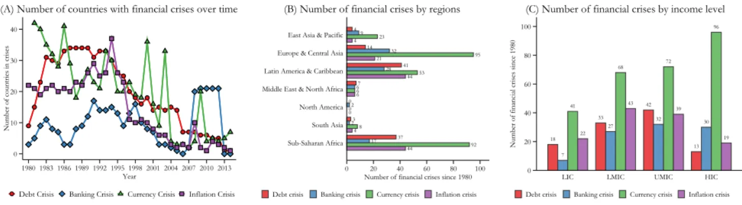
The evolution of financial crises during the period 1980-2014 can be summarized by the charts re-ported in Figure 1. According to (A), currency crises tend to occur more than other crises. Despite a downward trend in the number of countries affected by crises since the beginning of the 2000s, the 2008-09 contraction has been characterized by an increase in the incidence of banking, currency, and inflation crises. Moreover, as shown by (B), financial crises strike the economies by clusters and spread within the regions, with Europe & Central Asia, Latin America & Caribbean, and Sub-Saharan Africa being the most affected. Finally, (C) suggests that debt and inflation crises occur mostly in lower-middle, and upper-middle countries, currency crises are recorded more often in high-income countries, and banking crises are less recorded in low-income countries.
3.2.2 The connections between financial crises
We analyze potential connections between financial crises using the standard nonparametric Kaplan-Meier estimator. The main message of fig. 2 is that financial crises of a new type occur significantly quicker after a crisis of another type: (i) after a debt crisis hits a country, a banking or a currency crisis follows in one-quarter of cases in two years, and an inflation crisis in one year; (ii) after a banking crisis, a debt or a currency crisis follows in one-half of cases in three years, and an inflation crisis in two years; (iii) after a currency crisis, an inflation crisis follows in one-half of cases in one year, a debt crisis in two years, and a banking crisis in four years; and (iv) after an inflation crisis, a debt or a currency
Figure 1: Financial crises over time, by regions, and by income level 0 10 20 30 40
Number of countries in crises
1980 1983 1986 1989 1992 1995 1998 2001 2004 2007 2010 2013 Year
Debt Crisis Banking Crisis Currency Crisis Inflation Crisis
(A) Number of countries with financial crises over time
44 92 17 37 48 23 0 02 0 6 6 67 44 53 28 41 21 95 32 14 4 23 9 4 0 20 40 60 80 100 Number of financial crises since 1980 Sub-Saharan Africa
South Asia North America Middle East & North Africa Latin America & Caribbean Europe & Central Asia East Asia & Pacific
(B) Number of financial crises by regions
Debt crisis Banking crisis Currency crisis Inflation crisis
18 7 41 22 33 27 68 43 42 32 72 39 13 30 96 19 0 20 40 60 80 100
Number of financial crises since 1980
LIC LMIC UMIC HIC
(C) Number of financial crises by income level
Debt crisis Banking crisis Currency crisis Inflation crisis
Notes: Sample: 1980-2014. LIC, LMIC, UMIC, and HIC denote Low-, Lower-middle-, Upper-middle-, and High-income countries, respectively. Authors’
calculations based on data fromReinhart and Rogoff(2009) andLaeven and Valencia(2012), World Development Indicators, and Penn World Tables.
crisis follows in one-half of cases in three years, and a banking crisis in four years. Consequently, the takeaway for the design of our empirical analysis is that when estimating the effect of a crisis one should systematically control for other crises to avoid overestimating its trade cost.
3.2.3 Financial crises and international trade
As a foretaste of the potential trade costs of crises, fig. 3plots the cumulative change of trade flows from the year before the onset of each crisis to 5-year ahead. The overall picture supports the collapse of international trade. Total exports and imports decline sharply during all types of financial crises (for example, exports and imports decline respectively by around 20 and 32 percentage points of 2010 real GDP during a banking crisis), mainly driven by the contraction of trade in manufactured goods, followed by the one in services, mining goods, and agricultural goods. In sum, the trade costs of financial crises seem important. However, various issues may lead to an overestimation of these costs. Consequently, we develop in the following a formal econometric analysis to provide a robust estimation of the trade costs of financial crises.
4
Results
4.1
Estimation of propensity scores
As previously indicated, the first step of our analysis is devoted to the estimation of propensity scores (PS). Table 1 reports the marginal effects at the means of covariates in a pooled probit model for each type of crisis, and confirms that financial crises are not random but endogenous to several countries’
Figure 2: Survival models of the duration between the onset of different financial crises 0 .25 .5 .75 1
Probability of avoiding banking crisis 0 10 20 30
Duration (in year)
0 .25 .5 .75 1
Probability of avoiding currency crisis 0 10 20 30
Duration (in year)
0 .25 .5 .75 1
Probability of avoiding inflation crisis 0 10 20 30
Duration (in year)
(A) Probability of avoiding crises following a debt crisis
95% CI Survivor function 0 .25 .5 .75 1
Probability of avoiding debt crisis
0 5 10 15 20
Duration (in year)
0 .25 .5 .75 1
Probability of avoiding currency crisis 0 5 10 15 20
Duration (in year)
0 .25 .5 .75 1
Probability of avoiding inflation crisis 0 5 10 15 20
Duration (in year)
(B) Probability of avoiding crises following a banking crisis
95% CI Survivor function 0 .25 .5 .75 1
Probability of avoiding debt crisis
0 5 10 15 20
Duration (in year)
0 .25 .5 .75 1
Probability of avoiding banking crisis 0 5 10 15 20
Duration (in year)
0 .25 .5 .75 1
Probability of avoiding inflation crisis 0 5 10 15 20
Duration (in year)
(C) Probability of avoiding crises following a currency crisis
95% CI Survivor function 0 .25 .5 .75 1
Probability of avoiding debt crisis
0 10 20 30
Duration (in year)
0 .25 .5 .75 1
Probability of avoiding banking crisis 0 10 20 30
Duration (in year)
0 .25 .5 .75 1
Probability of avoiding currency crisis 0 10 20 30
Duration (in year)
(D) Probability of avoiding crises following an inflation crisis
95% CI Survivor function
Notes: The figure plots the estimated Kaplan-Meier survival functions for the duration between the start of one type of crisis and the start of another type of crisis. The y-axis denotes the compound probability that countries avoid crises. From the top row to the bottom row, we describe the probability of avoiding crises on y-axis following debt, banking, currency, and inflation crises, respectively. The bands are 95% confidence intervals. Authors’ calculations based on
Figure 3: Evolution of the average international trade in financial crises 2.9 4.7 11 7 26 2.7 1.42.23.5 9.8 0 5 10 15 20 25 No Debt crisis
(i) Debt crisis
3.14.5 10 6.9 25 1.3 .97 1.3 1.9 5.2 0 5 10 15 20 25 No Banking Crisis
(ii) Banking crisis
3.44.9 10 7.1 26 1.1 1.5 6.2 3.9 13 0 5 10 15 20 25 No Currency Crisis
(iii) Currency crisis
3.2 4.9 10 7 26 1.1 .43 4.6 3.2 9.4 0 5 10 15 20 25 No Inflation crisis
(iv) Inflation crisis Panel A: Exports (% of 2010 real GDP)
2.94.8 15 5.9 29 2.43.3 11 3 20 0 10 20 30 No Debt crisis
(i) Debt crisis
3.15 16 6 31 .32 .48 -.57 .014 -.21 0 10 20 30 No Banking Crisis
(ii) Banking crisis
3.35.4 16 6.1 31 1 .7 8 2.7 13 0 10 20 30 No Currency Crisis
(iii) Currency crisis
3 5.4 15 5.9 30 1.8 .25 9.5 2.1 14 0 10 20 30 No Inflation crisis
(iv) Inflation crisis Panel B: Imports (% of 2010 real GDP)
Agriculture Mining Manufacturing Services Total
Notes: The figure plots the dependent variables of our empirical models for the horizon h=5. The dependent variables are 100 times the cumulative change of agricultural, mining, manufacturing, services, and total exports and imports relative to the year prior to the onset of the crisis for years 1-5 after the onset of the crisis, scaled by 2010 real GDP. The dependent variables are plotted during debt, banking, currency, and inflation crises, and in the absence of crises. The first (second) row refers to exports (imports).
characteristics.12 Based on these models,fig. C.2 in Appendix Cillustrates the smooth kernel density of the distribution of the PS for the treated and control groups, for each financial crisis. Given the high classification power, countries in the treated (control) group receive a high (low) likelihood of financial crises, while countries in the treated (control) group with PS close to zero (one) receive higher weights. Besides, fig. C.2 also shows considerable overlaps between the distributions of PS for the treated and control groups; thus, we weighted the covariates using PS.13 As shown by tables C.6to C.9, according
to the criteria of Rubin (2002), weighting the covariates by the estimated PS eliminates most of the differences in covariates between the treated and the control group. Since our weighting strategy mimics a situation where financial crises occur randomly, it allows to properly identify the ATE of crises.
12In a nutshell, estimations show that: the likelihood of one crisis is increasing with the occurrence of other crises; banking and currency crises are most likely during economic booms but when economic growth decelerates; there is an inverted-U link between debt and inflation crises, and the level of development; the likelihood of debt and banking crises increases with the level of government debt and domestic credit; the likelihood of debt and inflation crises decreases with the terms of trade; the incidence of all types of crises decreases with the level of broad money in the economy; and currency crises are more likely in a floating exchange regime with a less independent central bank. Besides, standard diagnostic tests reported at the bottom of the table show that our models present a large classification power (above 85%) and Area Under Receiver Operating Characteristic curve (around 0.8 or more).
13FollowingImbens(2004) andCole and Hern´an(2008), we truncate the maximum weight to 10 to reduce the influence of outliers on our ATE estimates.
Table 1: Treatment models predicting the likelihood of financial crises, marginal effects
(1) (2) (3) (4)
Dependent variables Debt crisis (t) Banking crisis (t) Currency crisis (t) Inflation crisis (t)
Debt crisis (t-1) 0.009 (0.032) -0.006 (0.038) 0.054* (0.030)
Banking crisis (t-1) 0.028 (0.021) 0.112*** (0.031) 0.098*** (0.024)
Currency crisis (t-1) 0.060** (0.028) 0.077** (0.039) 0.119*** (0.034)
Inflation crisis (t-1) 0.004 (0.031) 0.097*** (0.030) 0.243*** (0.041)
Cyclical component of the log real GDP per capita (t-1) 0.055 (0.088) 0.459*** (0.145) 0.319*** (0.098) -0.148 (0.094)
Growth (average t-1 & t-2) -0.001 (0.001) -0.005*** (0.001) -0.004*** (0.001) 0.001 (0.001)
Log of real GDP per capita (t-1) 1.038*** (0.309) -0.046 (0.126) 0.094 (0.148) 0.421** (0.195)
Log of real GDP per capita squared (t-1) -0.065*** (0.020) 0.004 (0.007) -0.005 (0.009) -0.026** (0.011)
Public debt/GDP (t-1) 0.003*** (0.001) 0.001* (0.000) -0.000 (0.000) 0.000 (0.000)
Foreign reserves/GDP (t-1) -0.001 (0.002) -0.001 (0.002) 0.001 (0.002) -0.002 (0.002)
Domestic credit/GDP (t-1) 0.002** (0.001) 0.002*** (0.001) -0.000 (0.001) -0.002 (0.001)
Real exchange rate with US dollar (t-1) 0.000 (0.000) 0.000** (0.000) 0.000 (0.000) -0.000* (0.000)
Terms of trade (t-1) -0.371** (0.160) 0.044 (0.166) 0.104 (0.161) -0.341** (0.148)
Trade openness (t-1) 0.001 (0.001) 0.000 (0.000) -0.001 (0.001) -0.002*** (0.001)
Broad Money/GDP (t-1) -0.008*** (0.002) -0.001* (0.001) -0.002** (0.001) -0.004*** (0.001)
Current account/GDP (t-1) -0.003 (0.004) 0.004 (0.003) -0.002 (0.002) -0.003 (0.002)
Floating exchange regime dummy (t-1) 0.033 (0.033) -0.010 (0.033) 0.063** (0.026) 0.009 (0.030)
IMF Program dummy (t-1) 0.061*** (0.019) 0.112*** (0.031) -0.021 (0.027) -0.005 (0.022)
Central bank independence score (t-1) -0.054 (0.069) 0.084 (0.080) -0.282*** (0.095) -0.171 (0.115)
Intensity of conflicts measured by MEPV score (t-1) -0.010 (0.020) -0.004 (0.013) 0.007 (0.017) -0.000 (0.014)
Polity score (t-1) -0.000 (0.003) -0.003 (0.002) -0.002 (0.003) -0.000 (0.003)
Change in public debt/GDP (average t-1 & t-2) 0.001* (0.001) 0.001 (0.001) 0.002** (0.001) 0.000 (0.001)
Change in foreign reserves/GDP (average t-1 & t-2) 0.001* (0.000) 0.000 (0.000) -0.001*** (0.000) -0.000 (0.000)
Domestic credit/GDP (average t-1 & t-2) -0.001 (0.001) -0.000 (0.001) 0.000 (0.001) -0.001 (0.001)
Change in real exchange rate with US dollar (average t-1 & t-2) 0.000** (0.000) 0.000** (0.000) 0.000 (0.000) 0.000 (0.000)
Change in terms of trade (average t-1 & t-2) 0.003 (0.002) -0.001 (0.003) 0.003 (0.002) -0.001 (0.002)
Change in trade openness (average t-1 & t-2) -0.000 (0.001) -0.003** (0.001) 0.001 (0.001) 0.002* (0.001)
Change in broad Money/GDP (average t-1 & t-2) 0.001 (0.001) 0.000* (0.000) 0.001** (0.000) 0.002** (0.001)
Change in current account/GDP (average t-1 & t-2) 0.000 (0.000) -0.000 (0.000) -0.000 (0.000) 0.000 (0.000)
Observations 1262 1262 1262 1262
Classification 88.748 87.797 85.024 87.460
Model AUC 0.919 0.798 0.851 0.905
s.e. AUC 0.009 0.019 0.014 0.009
pseudo R2 0.435 0.189 0.296 0.394
Notes: Robust standard errors clustered at the country-level in parentheses. ∗p < 0.10, ∗ ∗ p < 0.05, ∗ ∗ ∗p < 0.01. Pooled probit model. The coefficients are
the marginal effects at the mean. AUC denotes Area Under Receiver Operating Characteristic curve.
4.2
Financial crises and aggregated trade
We first focus on aggregated trade, namely exports and imports, and then look at the trade balance. 4.2.1 Exports
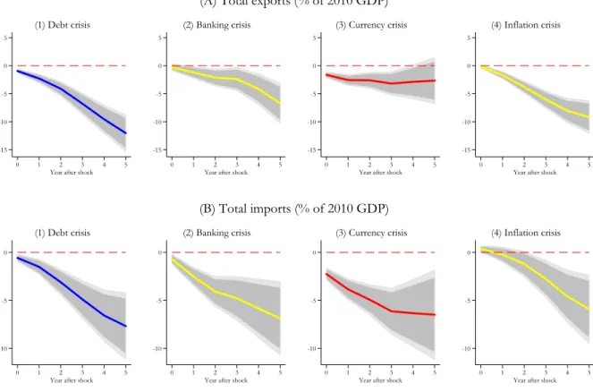
The ATE reported in column (1) oftable 2and the cumulative impulse response of AIPW estimates depicted by panel (A) offig. 4 show that financial crises reduce exports both on impact and cumulated over five years in countries affected by crises compared with those unaffected, except for currency crises whose effect on exports turns into not significant around year four. As shown byfig. 4, export costs are relatively small just after the occurrence of crises, but then intensify (with the exception of a U-pattern for currency crises). Finally, the magnitude of this negative effect is economically meaningful, ranging between a 12 percentage points (pp) contraction in terms of 2010 real GDP for debt crises, and 6.7 pp for banking crises.
Table 2: Cumulative trade costs over five years after financial crises
(I) Exports (II) Imports
(1) (2) (3) (4) (5) (6) (7) (8) (9) (10) Total Agri Mini Manu Serv Total Agri Mini Manu Serv Panel A: Debt crisis Panel E: Debt crisis
ATE -12.035*** 3.375*** -1.603 -8.039*** -1.599*** ATE -7.677*** 0.884*** -0.799** -7.058*** -0.694* (1.670) (0.696) (1.344) (0.985) (0.575) (1.764) (0.247) (0.374) (1.225) (0.359) Panel B: Banking crisis Panel F: Banking crisis
ATE -6.742*** 0.381 -1.657 -3.006** -2.507*** ATE -6.882*** -0.243 -0.165 -3.673*** -1.835*** (1.815) (0.813) (1.259) (1.347) (0.698) (1.956) (0.303) (0.463) (1.278) (0.500) Panel C: Currency crisis Panel G: Currency crisis
ATE -2.652 -0.674 -0.189 -0.270 -1.505** ATE -6.489*** -0.465 -0.911* -3.794*** -0.790 (2.100) (0.763) (1.781) (1.334) (0.767) (2.375) (0.391) (0.553) (1.466) (0.521) Panel D: Inflation crisis Panel H: Inflation crisis
ATE -9.171*** -0.531 -3.475*** -3.768*** 0.345 ATE -5.925*** 1.108*** -1.936*** -3.625*** -0.297 (1.491) (0.611) (1.124) (0.957) (0.599) (1.812) (0.345) (0.431) (1.101) (0.355) Observations 907 907 907 907 907 Observations 961 961 961 961 961 Notes: Robust standard errors clustered at the country-level in parentheses. ∗p < 0.10, ∗ ∗ p < 0.05, ∗ ∗ ∗p < 0.01. AIPW estimates. The dependent variables are 100 times the cumulative change of agricultural, mining, manufacturing, services, and total exports and imports relative to the year prior to the onset of the crisis for years 1-5 after the onset of the crisis, scaled by 2010 real GDP. Accumulated costs over five years. Restricted coefficients associated with controls to be equal for the treated and control groups. Observations in the treated and control groups are weighted by the propensity scores predicted in the treatment model. Maximum weights truncated at 10. Total denotes total trade of exports or imports; Agri denotes trade of agricultural goods; Mini denotes trade of mining goods; Manu denotes trade of manufactured goods; Serv denotes trade of services.
Figure 4: Cumulative trade costs over five years after financial crises
-15 -10 -5 0 5 0 1 2 3 4 5 Year after shock
(1) Debt crisis -15 -10 -5 0 5 0 1 2 3 4 5 Year after shock
(2) Banking crisis -15 -10 -5 0 5 0 1 2 3 4 5 Year after shock
(3) Currency crisis -15 -10 -5 0 5 0 1 2 3 4 5 Year after shock
(4) Inflation crisis
(A) Total exports (% of 2010 GDP)
-10 -5 0
0 1 2 3 4 5 Year after shock
(1) Debt crisis
-10 -5 0
0 1 2 3 4 5 Year after shock
(2) Banking crisis
-10 -5 0
0 1 2 3 4 5 Year after shock
(3) Currency crisis
-10 -5 0
0 1 2 3 4 5 Year after shock
(4) Inflation crisis
(B) Total imports (% of 2010 GDP)
Notes: Conditional cumulative change of total exports and imports from the start of the various crises (debt, banking, currency, and inflation crises). Each colored path shows local projections of the cumulative change relative to the year prior to the onset of the crisis for years 1-5 after the onset of the crisis.
These costs describe the difference in the change of trade between the treated and control groups after re-randomization using the predicted propensity scores.
4.2.2 Imports
The ATE reported in column (6) oftable 2and the cumulative impulse response of AIPW estimates depicted by panel (B) of fig. 4 confirm that imports are equally negatively affected by financial crises. Compared to their effect on exports, all types of crises exert significantly negative cumulated effects after five years, and only inflation crises do not significantly decrease imports in years one and two after their occurrence. Finally, similar to exports, the magnitude of the effect is important, ranging between a 7.7 pp of 2010 real GDP decrease over five years for debt crises, and 5.9 pp for inflation crisis.
4.2.3 Trade balance
We look at the costs of financial crises on the trade balance by comparing their costs on exports and imports (see table D.11 in Appendix D). Debt and inflation crises exert a negative effect on the trade balance over five years (around 4 pp of 2010 real GDP), due to the stronger decrease of exports compared with imports. Given their comparable negative effect on both exports and imports, banking crises are not found to significantly affect the trade balance five years after their burst. Finally, the trade balance improves following currency crises (by around 3.8 pp of 2010 real GDP), because of the absence of a significant effect on exports and the decline of imports.
Summing up, at the aggregated level we find that financial crises reduce the exports and imports of countries over five years. However, there are some differences across crises: (i) debt and inflation crises induce a higher reduction in exports than in imports, which deteriorates the trade balance; (ii) banking crises have comparable costs on exports and imports; (iii) currency crisis have no costs on exports but they reduce imports, which enhances the trade balance. Keeping these results in mind as a benchmark, we now look at the effects of financial crises at a more disaggregated level.
4.3
The trade costs of financial crises: getting granular
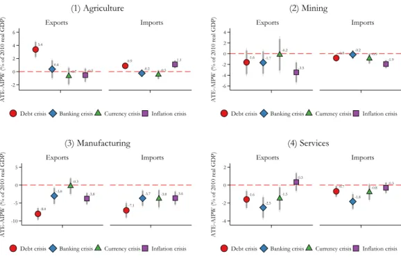
We now look at the costs of financial crises on the trade of agricultural, mining, and manufactured goods, and of services. As detailed in the introduction, this is, as far as we are aware, the first analysis that disentangles the aggregate trade costs of financial crises on all categories of goods and services traded. Estimated cumulative ATE over five years are reported intable 2, andfig. 5provides a graphical illustration.14
4.3.1 Agricultural trade
As shown by the panel (1) offig. 5, although financial crises mostly leave unchanged the exports and imports of agricultural goods, there are two important exceptions. Countries that experience debt crises
14To simplify the exposition, we focus hereafter on the cumulated costs over five years (the dynamics of the costs from the onset of the financial crises until five years ahead are available upon request).
Figure 5: Cumulative trade costs over five years after financial crises, granular level 3.4 0.4 -0.7 -0.5 0.9 -0.2 -0.5 1.1 -2 0 2 4 6 Exports Imports
Debt crisis Banking crisis Currency crisis Inflation crisis
ATE-AIPW (% of 2010 real GDP) (1) Agriculture -1.6 -1.7 -0.2 -3.5 -0.8 -0.2 -0.9 -1.9 -6 -4 -2 0 2 4 Exports Imports
Debt crisis Banking crisis Currency crisis Inflation crisis
ATE-AIPW (% of 2010 real GDP) (2) Mining -8.0 -3.0 -0.3 -3.8 -7.1 -3.7 -3.8 -3.6 -10 -5 0 5 Exports Imports
Debt crisis Banking crisis Currency crisis Inflation crisis
ATE-AIPW (% of 2010 real GDP) (3) Manufacturing -1.6 -2.5 -1.5 0.3 -0.7 -1.8 -0.8 -0.3 -4 -2 0 2 Exports Imports
Debt crisis Banking crisis Currency crisis Inflation crisis
ATE-AIPW (% of 2010 real GDP)
(4) Services
Notes: Robust standard errors clustered at the country-level in parentheses. ∗p < 0.10, ∗ ∗ p < 0.05, ∗ ∗ ∗p < 0.01. AIPW estimates. The dependent variables are 100 times the cumulative change of agricultural (1), mining (2), manufacturing (3), and services (4) exports and imports relative to the year prior to the onset of the crisis for years 1-5 after the onset of the crisis, scaled by 2010 real GDP. Accumulated costs over five years. Point estimates and confidence
intervals at 90% and 95% for the accumulated costs of the crises on international trade. Restricted coefficients associated with controls to be equal for the
treated and control groups. Observations in the treated and control groups are weighted by the propensity scores predicted in the treatment model. Maximum weights truncated at 10.
present larger exports and imports of agricultural goods by 3.4 and 0.9 pp of 2010 real GDP over five years respectively, compared with countries unaffected by crises. This is equally the case for imports in countries experiencing inflation crises (the effect equals 1.1 pp of 2010 real GDP). These findings suggest that trade in agricultural goods exhibits a great resilience during financial crises and can even intensify, which may signal a substitution effect in favor of agricultural goods.
4.3.2 Mining trade
The panel (2) of fig. 5 reveals that, except for inflation crises, the other financial crises do not sig-nificantly affect the exports of mining goods. However, countries affected by inflation crises experience a five-year cumulated loss of 3.5 pp of 2010 real GDP, which represents around 38% percent of the to-tal exports decrease. On the contrary, most financial crises significantly reduce the imports of mining goods, and the cumulative loss over five years in terms of 2010 real GDP ranges between 1.9 (0.8) pp for inflation (debt) crises, which represents around 33% (10%) of the total decrease of imports. Conse-quently, contrary to agricultural goods, trade in mining goods sometimes significantly declines following the occurrence of financial crises.
4.3.3 Manufacturing trade
Financial crises are systematically found to reduce the trade of exports and imports of manufactured goods (except for the lack of a significant effect of currency crises on exports). According to the panel (3) offig. 5, the magnitude of the effect is fairly important, ranging between 8 pp of 2010 real GDP for debt crisis and 3 pp for banking crises for exported manufactured goods (namely, between 67% and 45% of the total decrease of exports), and between 7.1 pp of 2010 real GDP for debt crises and 3.6 pp for inflation crises for imported manufactured goods (namely, between 92% and 61% of the total decrease of imports). However, despite being strongly affected by the occurrence of financial crises, the analysis of the trade of manufactured goods leaves unexplained between 8 and 55% of the trade costs at the aggregated level. 4.3.4 Services trade
Finally, the panel (4) infig. 5displays the results for the trade of services. Similar with manufacturing trade, services trade is significantly reduced by the most types of financial crises. Indeed, with the exception of inflation and currency crises for imports, and inflation crises for exports, both services exports and imports significantly decline. Yet again, the effect is sizable, ranging between 2.5 pp of 2010 real GDP for banking crises and 1.5 pp for currency crises for services exports (namely, between 37% and 57% of the total decrease in exports), and between 1.8 pp of 2010 real GDP for banking crises and 0.7 pp for debt crises for services imports (namely, between 27% and 9% of the total decrease in imports).
To summarize, our granular analysis reveals that, while manufactured traded goods are the most affected in terms of magnitude, the impact of financial crises on the other types of traded goods and on services is far from being negligible. Trade in both mining goods and services significantly declines following several types of financial crises, while trade in agricultural goods seems to benefit from a possible substitution effect particularly following debt crises.
4.4
The trade costs of combined financial crises
The analysis performed so far focused on the effect of each financial crisis, when controlling for the other types of crises in the prediction of the potential outcome and in the computation of propensity scores. Given that financial crises seem to be connected (see the previous section), we now look at the trade effects of combined crises. However, our methodology of impact assessment and local projections does not allow seizing the effect of combined crises using interactive terms. Consequently, we draw upon a total of eleven dummy variables that define double, triple, and quadruple crises occurring in a given country. FollowingGlick and Hutchison(2001) andHutchison and Noy(2005), these dummies are based on a two-year band around single financial crises, such as a combined crisis occurs if, given a crisis that spans between t and t+ T, another type of crisis occurs in any of the years spanning between t − 2 and t+ T + 2. In this case, our dummy variable is equal to one from the beginning of the first crisis until the
end of the last crisis. In addition, we remove from the control group all country-year observations with at least one crisis to ensure that countries in this group did not experience any crisis.
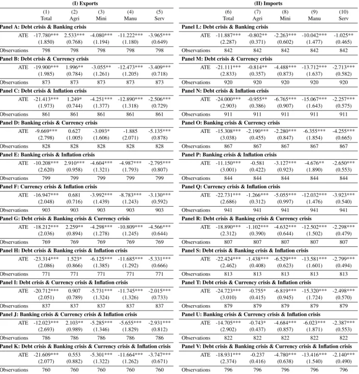
The results reported in table 3show that combined financial crises trigger more significant and of a higher magnitude aggregated trade costs. Indeed, equality tests show that the trade effects of combined crises are statistically higher than those of a single crisis (see tables D.12andD.13). For instance, the five-year cumulated ATE measuring the decline of total exports for the 44 cases of quadruple crises equals 21.6 pp of 2010 real GDP (see the bottom oftable 3), namely well above their individual effect (equal to 12 pp, 6.7 pp, and 9.2 pp for debt, banking, and inflation crises, respectively).
Going granular,table 3reveals that the magnitude of the decline of the trade of manufactured goods due to combined crises is reinforced compared with a single crisis, as the effect is above 10 pp of 2010 real GDP in most cases (in 15 out of 22 estimated ATE, see columns 4 and 9 intable 3). Moreover, combined financial crises always significantly reduce the trade of mining goods and services (all estimated 44 ATE are negative and significant in columns 3, 5, 8, and 10). Finally, as illustrated by table 3, most combined financial crises significantly reduce agricultural goods imports (9 out of 11 ATE are negative and significant in column 7), and foster agricultural goods exports (7 out of 11 ATE are positive and significant in column 2). Altogether, results based on combined financial crises unveil more severe trade costs.
5
Robustness
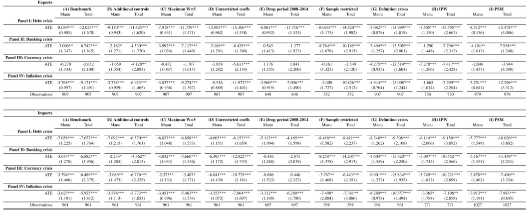
We further investigate the robustness of our findings using a wide variety of alternative specifications. To save space, we report intable 4only the trade costs of aggregated exports and imports, and manufac-turing trade. The results for agricultural and mining trade, and for combined crises are available upon request.
5.1
Additional controls in the outcome model
We draw upon additional controls to reduce a potential bias related to omitted variables. To this end, we extend the common number of variables of the treatment and outcome models by adding in the latter the average (computed over two years lags) of the change in public debt, foreign reserves, domestic credit, real exchange rate with the US dollar, terms of trade, trade openness, broad money, and current account. As illustrated by column B intable 4, except for the effect of currency crises on total exports that is now significant (a decrease of 4.1 pp of 2010 real GDP in the countries affected by currency crises), accounting for additional controls leaves our main results qualitatively unchanged.
Table 3: Cumulative trade costs over five years after financial crises, combined crises
(I) Exports (II) Imports
(1) (2) (3) (4) (5) (6) (7) (8) (9) (10)
Total Agri Mini Manu Serv Total Agri Mini Manu Serv
Panel A: Debt crisis & Banking crisis Panel L: Debt crisis & Banking crisis
ATE -17.780*** 2.533*** -4.080*** -11.222*** -3.965*** ATE -11.887*** -0.802** -2.263*** -10.042*** -1.025**
(1.850) (0.768) (1.194) (1.180) (0.649) (2.287) (0.371) (0.602) (1.477) (0.465)
Observations 798 798 798 798 798 Observations 842 842 842 842 842
Panel B: Debt crisis & Currency crisis Panel M: Debt crisis & Currency crisis
ATE -19.900*** 1.996** -3.055** -12.473*** -3.409*** ATE -21.111*** -0.814** -4.488*** -13.712*** -2.713***
(1.985) (0.784) (1.261) (1.205) (0.718) (2.833) (0.357) (0.873) (1.637) (0.582)
Observations 873 873 873 873 873 Observations 920 920 920 920 920
Panel C: Debt crisis & Inflation crisis Panel N: Debt crisis & Inflation crisis
ATE -21.413*** 1.249* -4.251*** -12.890*** -2.506*** ATE -24.000*** -0.955** -6.765*** -15.067*** -2.257***
(1.973) (0.744) (1.377) (1.318) (0.729) (2.903) (0.386) (0.907) (1.643) (0.575)
Observations 861 861 861 861 861 Observations 911 911 911 911 911
Panel D: Banking crisis & Currency crisis Panel O: Banking crisis & Currency crisis
ATE -9.669*** 0.627 -3.093* -1.885 -5.135*** ATE -15.308*** -2.190*** -2.280*** -6.355*** -4.255***
(2.798) (1.005) (1.606) (2.071) (0.878) (3.038) (0.455) (0.847) (1.854) (0.665)
Observations 828 828 828 828 828 Observations 867 867 867 867 867
Panel E: Banking crisis & Inflation crisis Panel P: Banking crisis & Inflation crisis
ATE -10.208*** 2.910*** -4.604*** -4.987*** -2.795*** ATE -11.150*** -0.581 -3.127*** -4.676** -2.650***
(2.620) (0.958) (1.321) (1.793) (0.807) (3.001) (0.422) (0.923) (1.890) (0.553)
Observations 799 799 799 799 799 Observations 844 844 844 844 844
Panel F: Currency crisis & Inflation crisis Panel Q: Currency crisis & Inflation crisis
ATE -16.947*** 0.681 -3.992*** -8.783*** -3.130*** ATE -22.731*** -1.266*** -5.055*** -12.032*** -3.923***
(2.048) (0.716) (1.439) (1.243) (0.592) (2.686) (0.312) (0.997) (1.476) (0.540)
Observations 903 903 903 903 903 Observations 941 941 941 941 941
Panel G: Debt crisis & Banking crisis & Currency crisis Panel R: Debt crisis & Banking crisis & Currency crisis
ATE -18.212*** 2.259** -4.298*** -10.809*** -4.566*** ATE -18.890*** -1.102*** -4.632*** -12.502*** -2.298***
(2.036) (0.894) (1.278) (1.245) (0.644) (2.312) (0.390) (0.644) (1.502) (0.479)
Observations 769 769 769 769 769 Observations 807 807 807 807 807
Panel H: Debt crisis & Banking crisis & Inflation crisis Panel S: Debt crisis & Banking crisis & Inflation crisis
ATE -23.314*** 1.523* -6.125*** -11.685*** -5.331*** ATE -22.424*** -1.438*** -6.529*** -13.581*** -2.799***
(2.086) (0.866) (1.385) (1.292) (0.666) (2.462) (0.408) (0.623) (1.601) (0.494)
Observations 771 771 771 771 771 Observations 813 813 813 813 813
Panel I: Debt crisis & Currency crisis & Inflation crisis Panel T: Debt crisis & Currency crisis & Inflation crisis
ATE -20.712*** 0.907 -5.731*** -11.745*** -2.015*** ATE -24.723*** -0.755* -6.819*** -15.320*** -2.498***
(2.051) (0.789) (1.324) (1.326) (0.733) (3.010) (0.415) (0.945) (1.724) (0.570)
Observations 837 837 837 837 837 Observations 879 879 879 879 879
Panel J: Banking crisis & Currency crisis & Inflation crisis Panel U: Banking crisis & Currency crisis & Inflation crisis
ATE -12.023*** 2.103** -5.285*** -5.655*** -2.931*** ATE -14.705*** -0.743* -4.684*** -6.023*** -2.387***
(2.693) (0.989) (1.346) (1.829) (0.812) (2.902) (0.437) (0.857) (1.871) (0.553)
Observations 786 786 786 786 786 Observations 822 822 822 822 822
Panel K: Debt crisis & Banking crisis & Currency crisis & Inflation crisis Panel V: Debt crisis & Banking crisis & Currency crisis & Inflation crisis
ATE -21.609*** 0.553 -5.301*** -11.664*** -3.747*** ATE -18.931*** -0.237 -4.780*** -13.416*** -2.140***
(2.077) (0.882) (1.322) (1.262) (0.671) (2.374) (0.416) (0.638) (1.540) (0.490)
Observations 760 760 760 760 760 Observations 796 796 796 796 796
Notes: Robust standard errors clustered at the country-level in parentheses. ∗p < 0.10, ∗ ∗ p < 0.05, ∗ ∗ ∗p < 0.01. AIPW estimates. The dependent variables are 100 times the cumulative change of agricultural, mining, manufacturing, services, and total exports and imports relative to the year prior to the onset of the crisis for
years 1-5 after the onset of the crisis, scaled by 2010 real GDP. Accumulated costs over five years. Restricted coefficients associated with controls to be equal for
the treated and control groups. Observations in the treated and control groups are weighted by the propensity scores predicted in the treatment model. Maximum weights truncated at 10. Total denotes total trade of exports or imports; Agri denotes trade of agricultural goods; Mini denotes trade of mining goods; Manu denotes trade of manufactured goods; Serv denotes trade of services.
5.2
Alternative assumptions
Compared to the maximum weight of 10 for our treated and control groups used in the benchmark model, we now use a maximum weight of 5 to reduce the influence of country-year observations in the treated (control) group that receive a low (high) likelihood of financial crises. Results reported in column C of intable 4confirm the robustness of the significance and the size of the effect of financial crises on total and manufacturing trade. Moreover, we relax the assumption of an identical impact of covariates in the outcome model for the treated and control groups. As such, in addition to financial crises, covariates are now equally allowed to impact international trade differently during and outside financial crises. As shown by column D, except for the significant (not significant) effect of currency (inflation) crises on total (manufacturing) exports, relaxing this restriction yields results that are comparable with our benchmark findings.
5.3
Sample selection
We alter the benchmark sample in two ways. First, we drop the period from 2008 onwards, given the collapse in international trade and the rise of banking, currency, and inflation crises. Removing this period does not affect our main results for debt and inflation crises. However, adding to our previous analysis, results in column E intable 4show that the events that occurred during this period are indeed an important driver of the trade effects of banking crises (their effect on both total and manufacturing trade is no longer significant starting around year two, see fig. D.3), and, to some extent, of currency crises (their effect on imports is no longer significant starting around year four, seefig. D.3). Second, following
Trebesch and Zabel(2017), we increase the homogeneity of our sample by removing small countries (i.e. with a population below one million at the end year of our sample) and developed countries. Estimations reported in column F confirm our benchmark results, except for the loss of significance in the effect of inflation crises on manufacturing exports.
5.4
Alternative sources and definitions of crises
We consider alternative sources and definitions of financial crises. Following Cruces and Trebesch
(2013), debt crises now exclusively capture debt restructurings with private creditors (i.e. we drop re-structurings with official creditors). Banking crises have the same definition but now come from the dataset of Reinhart and Rogoff(2009) (instead ofLaeven and Valencia, 2012). Currency crises are re-defined based on Frankel and Rose(1996), namely by at least a 25% nominal depreciation of the local currency against the US dollar that is also at least a 10% increase in the rate of depreciation. Finally, inflation crises are signalled by inflation rates of 40% or more, followingBruno and Easterly(1998) and
Reinhart and Rogoff(2009). Except for the effect of currency crises on total and manufacturing exports that is now significant, results in column G oftable 4are consistent with our benchmark findings.
5.5
Alternative ATE estimators
Compared with our benchmark analysis that draws upon the Augmented Inverse Propensity Weighted (AIPW) estimator, we use alternative methods that are popular in the existing literature, namely the In-verse Propensity Weighting (IPW) and the Propensity score matching (PSM). As illustrated by columns H and I intable 4, the use of these alternative estimators confirms our main findings,15 except now
cur-rency crises significantly reduce total and manufacturing exports, and the effect of banking and inflation crises on manufacturing exports is no longer significant when using the IPW.
5.6
Placebo crises
Finally, we look if our results are not spurious and driven by the employed methodology. To this end, we drop all country-year observations with financial crises, and randomly assign the same number and duration of crises to the remaining sample that never experienced a financial crisis. Results based on repeating this procedure 500 times are reported intable 5, and show that the percentage of significant ATE estimates for the trade costs is fairly low (always below 10%, and only in 6 out of 80 cases above 5%). This finding supports, yet again, the robustness of our benchmark findings.
6
Sensitivity
As previously emphasized, our results are confirmed by several robustness tests. In the following, we explore whether the trade costs of financial crises differ with respect to several key structural characteris-tics of countries. Tables 6to10report the cumulated trade costs over five years.
6.1
The level of development
We look at the trade costs of financial crises at various levels of development. Indeed, the level of development is related to the structure of the economy, including specialization, and diversification of exports and imports, as well as its resilience to shocks, including financial crises. To this end, we draw upon the average real GDP per capita over 1980-2014, and define three groups corresponding to low-, middle-, and high-income countries.16 Table 6provides the results for each group of countries, provided
15PSM is performed with five neighbors, and we report that estimations with an alternative number of neighbors are com-parable (results are available upon request).
16The two thresholds separating the three groups are set at 3,000 and 10,000 USD, as these levels take into account coun-tries’ specialization according to the types of goods and services they export (import) to (from) the rest of the world. In particular, the use of the average real GDP per capita may better capture income dynamics compared with a single year gross national income per capita (see, for example, World Bank’s classification). The list of countries by level of development is reported intable D.10inAppendix D. We report that variations in the threshold values did not reveal qualitative changes in our findings. In addition, using other indicators of development, such as the human development index or the economic complexity index to define the income groups, leads to comparable findings (results are available upon request).
Table 4: Robustness checks, cumulative trade costs over five years after financial crises, total and manufacturing trade (exports and imports)
Exports
(A) Benchmark (B) Additional controls (C) Maximun W=5 (D) Unrestricted coeffs (E) Drop period 2008-2014 (F) Sample restricted (G) Definition crises (H) IPW (I) PSM Manu Total Manu Total Manu Total Manu Total Manu Total Manu Total Manu Total Manu Total Manu Total Panel I: Debt crisis
ATE -8.039*** -12.035*** -9.170*** -11.425*** -7.918*** -11.739*** -13.903*** -15.306*** -8.081*** -11.716*** -10.643*** -14.420*** -7.082*** -14.999*** -7.505*** -13.795*** -8.512*** -15.478*** (0.985) (1.670) (0.943) (1.620) (0.931) (1.471) (0.962) (1.538) (0.932) (1.524) (1.175) (1.982) (0.879) (1.819) (1.150) (2.667) (0.136) (4.086) Panel II: Banking crisis
ATE -3.006** -6.742*** -2.182* -4.530*** -3.992*** -7.117*** -3.189** -8.429*** 0.543 -1.377 -8.764*** -10.185*** -3.494*** -13.505*** -1.290 -7.796*** -4.101** -7.938*** (1.347) (1.815) (1.271) (1.720) (1.074) (1.449) (1.291) (1.740) (1.413) (1.933) (1.676) (2.915) (1.257) (2.001) (1.448) (2.313) (1.613) (1.248) Panel III: Currency crisis
ATE -0.270 -2.652 -1.659 -4.120** -0.432 -1.767 -1.858 -5.613*** 1.176 1.041 -0.161 -2.549 -4.275*** -12.519*** -3.270*** -7.417*** -2.046 -3.944 (1.334) (2.100) (1.354) (2.083) (1.067) (1.615) (1.282) (2.134) (1.535) (2.200) (1.325) (2.120) (0.935) (1.604) (1.266) (2.428) (1.437) (4.398) Panel IV: Inflation crisis
ATE -3.768*** -9.171*** -2.778*** -6.923*** -3.837*** -9.274*** -0.516 -11.972*** -3.960*** -7.006*** -2.400 -10.826*** -4.944*** -12.008*** -1.665 -7.299*** -5.251*** -12.296*** (0.957) (1.491) (0.929) (1.465) (0.936) (1.367) (0.889) (1.401) (0.915) (1.490) (1.727) (2.512) (0.764) (1.244) (1.014) (2.264) (0.841) (3.312) Observations 907 907 907 907 907 907 907 907 648 648 352 352 907 907 730 730 979 979
Imports
(A) Benchmark (B) Additional controls (C) Maximun W=5 (D) Unrestricted coeffs (E) Drop period 2008-2014 (F) Sample restricted (G) Definition crises (H) IPW (I) PSM Manu Total Manu Total Manu Total Manu Total Manu Total Manu Total Manu Total Manu Total Manu Total Panel I: Debt crisis
ATE -7.058*** -7.677*** -7.092*** -6.570*** -6.837*** -6.858*** -4.605*** -6.153*** -5.113*** -4.165*** -8.418*** -9.411*** -8.248*** -9.308*** -6.114*** -9.150*** -5.777*** -10.026*** (1.225) (1.764) (1.215) (1.761) (1.048) (1.533) (1.151) (1.659) (1.094) (1.598) (1.582) (2.237) (1.262) (2.108) (2.066) (3.092) (1.549) (3.802) Panel II: Banking crisis
ATE -3.673*** -6.882*** -2.233* -4.362** -4.042*** -5.660*** -6.495*** -12.822*** -0.436 -2.875 -8.258*** -14.205*** -7.604*** -15.620*** -5.097*** -10.552*** -5.167*** -11.439*** (1.278) (1.956) (1.285) (2.013) (1.034) (1.556) (1.172) (1.733) (1.288) (2.019) (1.378) (2.913) (1.559) (2.250) (1.744) (2.566) (1.551) (2.251) Panel III: Currency crisis
ATE -3.794*** -6.489*** -3.689** -6.776*** -2.373** -3.407* -6.041*** -10.729*** -0.686 -0.446 -3.767** -6.443*** -9.901*** -15.834*** -5.745*** -10.221*** -3.878*** -7.496** (1.466) (2.375) (1.473) (2.325) (1.133) (1.771) (1.439) (2.181) (1.522) (2.327) (1.468) (2.351) (1.227) (1.935) (1.817) (2.899) (1.462) (3.324) Panel IV: Inflation crisis
ATE -3.625*** -5.925*** -3.586*** -5.773*** -3.451*** -5.463*** -3.355*** -7.864*** -3.112*** -6.280*** -3.498* -7.381** -8.280*** -10.557*** -3.365* -7.106** -3.913*** -7.983*** (1.101) (1.812) (1.113) (1.853) (0.996) (1.534) (1.072) (1.697) (1.109) (1.780) (2.084) (3.086) (0.978) (1.494) (1.784) (2.858) (1.191) (0.845) Observations 961 961 961 961 961 961 961 961 697 697 398 398 961 961 771 771 1027 1027 Robust standard errors clustered at the country-level in parentheses. ∗p < 0.10, ∗ ∗ p < 0.05, ∗ ∗ ∗p < 0.01. AIPW estimates. The dependent variables are 100 times the cumulative change of manufacturing, and total exports and imports relative to the year prior to the onset of the crisis for years 1-5 after the onset of the crisis, scaled by 2010 real GDP. Accumulated costs over five years. Column (A): benchmark results. Column (B): additional controls. Column (C): maximum weight set to 5. Column (D): unrestricted coefficients. Column (E): drop the period 2008-2014; Column (F): drop of small and developed countries. Column (G): change the definitions and sources of crises. Column (H): Inverse propensity weighting (IPW) estimator. Column (I): Propensity score matching (PSM) estimator.