HAL Id: inserm-00624053
https://www.hal.inserm.fr/inserm-00624053
Submitted on 15 Sep 2011
HAL is a multi-disciplinary open access
archive for the deposit and dissemination of
sci-entific research documents, whether they are
pub-lished or not. The documents may come from
teaching and research institutions in France or
abroad, or from public or private research centers.
L’archive ouverte pluridisciplinaire HAL, est
destinée au dépôt et à la diffusion de documents
scientifiques de niveau recherche, publiés ou non,
émanant des établissements d’enseignement et de
recherche français ou étrangers, des laboratoires
publics ou privés.
Transmission of distributed deterministic telporal
information through a diverging/converging three-layers
neural network
Yoshiyuki Asai, Alessandro Villa
To cite this version:
Yoshiyuki Asai, Alessandro Villa. Transmission of distributed deterministic telporal information
through a diverging/converging three-layers neural network. 20th International Conference on
Ar-tificial Neural Networks, Sep 2011, Thessaloniki, Greece. pp.145-154. �inserm-00624053�
Transmission of distributed deterministic
temporal information through a
diverging/converging three-layers neural network
Yoshiyuki Asai1,2,3 and Alessandro E. P. Villa2,3
1
The Center for Advanced Medical Engineering and Informatics, Osaka University, Osaka, Japan
2 INSERM U836; Grenoble Inst. of Neuroscience; Universit´e Joseph Fourier, Neuro
Heuristic Research Group, Eq. 7 - Nanom´edecine et Cerveau, Grenoble, France
Neuro Heuristic Research Group, Information Science Institute, University of Lausanne, Lausanne, Switzerland
http://www.neuroheuristic.org/
Abstract. This study investigates the ability of a diverging/converging
neural network to transmit and integrate a complex temporally orga-nized activity embedded in afferent spike trains. The temporal infor-mation is originally generated by a deterministic nonlinear dynamical system whose parameters determine a chaotic attractor. We present the simulations obtained with a network formed by simple spiking neurons (SSN) and a network formed by a multiple-timescale adaptive threshold neurons (MAT). The assessment of the temporal structure embedded in the spike trains is carried out by sorting the preferred firing sequences detected by the pattern grouping algorithm (PGA). The results suggest that adaptive threshold neurons are much more efficient in maintain-ing a specific temporal structure distributed across multiple spike trains throughout the layers of a feed-forward network.
Key words: spiking neural networks, synfire chains, adaptive threshold
neurons, computational neuroscience, preferred firing sequences
1
Introduction
A neuronal network can be considered as a highly complex nonlinear dynamical system able to exhibit deterministic chaotic behavior, as suggested by the ex-perimental observations of single unit spike trains, which are sequences of the exact timing of the occurrences of action potentials [1, 2]. Previous studies [3, 4] showed that deterministic nonlinear dynamics in noisy time series could be detected by applying algorithms aimed at finding preferred firing sequences with millisecond order time precision from simultaneously recorded neural activities. A neural network is also characterized by the presence of background activity of unspecified or unknown origin that is often represented by stochastic inputs to
each cell of the network. Then, a neuron belonging to a cell assembly, somehow associated to a deterministic nonlinear system, within the network is expected to receive inputs characterized by an embedded temporal structure as well as inputs corresponding to the stochastic background activity. It has been shown that the characteristic transfer function of a neuronal model and the statistical feature of the the background activity may affect the transmission of temporal information through synaptic links [5].
In the current paper we extend our previous analysis to diverging/converging feed-forward neuronal networks–synfire chains–which are supposed to represent the most appropriate circuits able to transmit information with the best tem-poral accuracy [6]. Moreover the temtem-porally organized activity was fed to the network in a distributed way across the input spike trains [7]. We suggest that adaptive threshold neurons are much more efficient in maintaining a specific temporal structure throughout the layers of a synfire chain.
2
Methods
2.1 Spiking neuron model
We investigated two neuron models aimed to reproduce the dynamics of regular spiking neurons. The first is a simple spiking neuron (SSN) [8] described as:
dv dt = 0.04v 2+ 5v + 140− u + I ext(t) , (1) du dt = a(bv− u) ,
with the auxiliary after-spike resetting, v← c and u ← u+d when v ≥ +30 mV .
v represents the membrane potential [mV ], u is a membrane recovery variable, a and b control the time scale of the recovery variable and its sensitivity to the subthreshold fluctuation of the membrane potential. This model generates an action potential with a continuous dynamics followed by a hyperpolarization modeled as a discontinuous resetting. Parameters were set as a = 0.02, b = 0.2,
c =−65, d = 8 so to mimic the behavior of a regular spiking neuron [8].
The second model is a multiple-timescale adaptive threshold (MAT) model [9] derived from [10]. In this model, the dynamics of the membrane potential is described as a non-resetting leaky integrator,
τm
dV
dt =−V + R A Iext(t) , (2)
where τm, V, R and A are the membrane time constant, membrane potential,
membrane resistance, and scaling factor, respectively. A spike is generated when the membrane potential V reaches the adaptive spike threshold θ(t),
θ(t) = ω + H1(t) + H2(t) ,
dH1
dt =−H1/τ1 , (3)
dH2
Temporal information distributed across multiple spike trains 3
where ω is the resting value, H1 and H2 are components of the fast and slow
threshold dynamics (characterized by decaying time constants τ1and τ2, respec-tively) which has a discrete jump when V (t)≥ θ(t),
H1= H1+ α1, H2= H2+ α2 . (4)
Parameters were set to values τm= 5 ms, R = 50 MΩ, A = 0.106, ω = 19 mV,
τ1= 10 ms, τ2= 200 ms, α1 = 37 mV, α2= 2 mV. The model with the above
parameter values reproduces the activity of a regular spiking neuron [9]. Let us denote Iext the input synaptic current, defined as
Iext=−Aext
∑
k
gsyn(t− tk) , (5)
where Aext is an intensity of the synaptic transmission of the spike received as
an external input (Aext= 1 was used here for all simulations), tkrepresents time
when the k-th spike arrives to the neuron model, and gsyn is the post synaptic
conductance represented by gsyn(t) = C0 e−t/˜τ1− e−t/˜τ2 ˜ τ1− ˜τ2 , (6)
where ˜τ1 and ˜τ2 are rise and decay time constants given by 0.17 and 4 ms,
respectively, and C0 is a coefficient used to normalize the maximum amplitude
of gsyn(t) to 1. Notice that a single synaptic current given to a neuron is not
strong enough to evoke post-synaptic neuronal discharges. Hence, it is necessary for a post-synaptic neuron to integrate several arriving synaptic currents for a spike generation.
2.2 Input spike train
We consider the deterministic dynamical system described by Zaslavskii [11]: {
xn+1= xn+ v(1 + µyn) + εvµ cos xn , (mod. 2π)
yn+1= e−γ(yn+ ε cos xn) ,
(7)
where x, y, µ, v ∈ R, the parameters are µ = 1−eγ−γ, v = 4003 and initial condi-tions set to x0= y0= 0.3. With this parameter set the system exhibits a chaotic
behavior. Time series {xn} are generated by iterative calculation. A new time
series{wn} corresponding to the sequence of the inter-spike-intervals is derived
by wn = xn+1− xn+ C, where C = min{(xn+1− xn)} + 0.1 is a constant to
make sure wn > 0. The dynamics was rescaled in milliseconds time units with
an average rate of 5 events/s (i.e., 5 spikes/s) in order to let the mean rate of the Zaslavskii spike train be comparable to neurophysiological experimental
data. We calculated N = 10000 points of time series{wn} which corresponds to
a spike train lasting L = 2000 seconds.
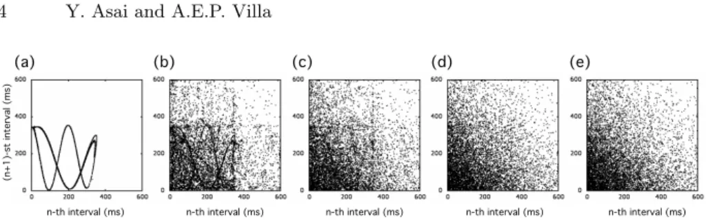
Given a dynamical information ratio D, where 0 ≤ D ≤ 1, a percentage
(a) (b) (c) (d) (e)
n-th interval (ms)
(n+1)-st interval (ms)
n-th interval (ms) n-th interval (ms) n-th interval (ms) n-th interval (ms)
Fig. 1. Return maps of input spike trains with an average rate of 5 spikes/s as a
function of the dynamical information ratio (D). The (n + 1)-st inter-spike-interval are plotted against the n-th inter-spike-interval. The axes are scaled in ms time units. (a)
D = 1, (b) D = 0.7, (c) D = 0.5, (d) D = 0.3, (e) D = 0.
distributed) and deleted from the initial Zaslavskii spike train, thus yielding a sparse Zaslavskii spike train. Then, the sparse Zaslavskii spike train is merged
with a Poissonian spike train with mean firing rate N (1− D)/L spikes/s, thus
yielding an input spike train with an average rate close to 5 spikes/s and a duration of 2000 s. In case of overlapping spikes only one event is kept in the input spike train. Notice that if D = 1 all input spike trains are identical to the original Zaslavskii spike train and if D = 0 all input spike trains are independent Poissonian spike trains. For a given dynamical information ratio D this procedure is repeated 20 times such to provide 20 different input spike trains. In the current simulations the dynamical information ratio ranged from 0 to 1.0 with 0.1 steps. Return maps of input spike trains are shown in Fig. 1.
2.3 Neuronal network
We consider a diverging/converging neural network composed of three layers (Fig. 2). Each layer includes 20 neurons characterized by the same neuronal model with identical parameter values. Each neuron belonging to the first layer receives fifteen input spike trains randomly selected out of the twenty that were generated for a given dynamical information ratio D. Hence, a neuron in the first layer receives afferences from 15 input spike trains (each one firing on average at = 5 spikes/s) and an independent Poissonian spike train with a mean firing rate of 425 spikes/s as background activity. This means a neuron of the first layer integrates about 500 spikes in 1000 millisecond by the fourth order Runge-Kutta numerical integration method with 0.01 ms time steps. Each neuron of the next layer receives afferences from 15 neurons randomly selected in the previous layer. In addition, each neuron receives an independent Poissonian spike train with a mean firing rate of 425 spikes/s as background activity. We observed that those neurons integrated between 490 and 540 spikes in 1000 ms The explicit synaptic transmission delay is not considered here. All connections were hardwired, and no synaptic plasticity was taken into account. Each simulation run lasted 2000 s.
Temporal information distributed across multiple spike trains 5 PST PST | | | | || | | | | | | || | | | | | | | | || | | | | | | | | | || | | | | | | | | | | | ||| || | | | || || || | | | | |
Input Spike Train 1
Input Spike Train 2
Input Spike Train 3
20 cells Layer 1 1 2 3 PST PST 20 cells Layer 2 PST 1 2 3 20 cells Layer 3 PST 1 2 3 PST PST || | || | ||| | | ||| ||| | | || | |
Input Spike Train 20
20 PST 20 PST 20 PST PST | | | | || | || | | | || | | | | || |
Original Zaslavskii Spike Train
Fig. 2. Convergent/divergent feed-forward circuit formed by three neuron layers. Each
cell receives 15 afferent spike trains randomly selected out of 20 and a PST (independent Poissonian spike train).
2.4 Pattern detection and reconstruction of time series
Subsets of spike trains were obtained by using the Pattern Grouping Algorithm (PGA) [12–14] as follows. Firing sequences repeating at least 5 times and above the chance level (p = 0.05) are detected by PGA. The interval between the first and the last spike of the firing sequence defines the duration of the pattern
that was set to ≤ 600 ms. Given a maximum allowed jitter in spike timing
accuracy (±3 ms) clusters of firing sequences are represented by a template
pattern. For example, if there are 9 triplets (i.e., firing sequences formed by 3 spikes) belonging to the same cluster, a subset of the original spike train that
includes 27 spikes (= 9× 3) can be determined by a template pattern. Then,
the subset of the original spike train referred to as “reconstructed spike train” is obtained by pooling all spikes belonging to all template pattern clusters [4]. The reconstructed spike train from the original Zaslavskii series included 92.3% of the original spikes and its return map is shown in Fig. 3a. In a case of a Poissonian spike train with an average rate of 5 spikes/s the reconstructed spike train included only 0.4% spikes of the original series (Fig. 3b).
Moreover, we have measured the dispersion of spike distribution by the Fano factor [15], which is F = 1 for a Poissonian spike train, and the similarity ratio S between two spike trains defined as follows. Suppose that spike trains A and
B contain NA and NB spikes and M spikes occur in A and B at the same
time. The similarity ratio is defined by S = 2M/(NA+ NB), which is S = 1 for
two identical spike trains. If we allow the coincidence to occur within a given jitter (∆ = 5 ms here), then the condition tnB− ∆ ≤ tkA ≤ tnB+ ∆ satisfies the coincidence of the n-th spike in train B with the k-th spike in train A.
(a) (b)
n-th interval (ms) n-th interval (ms)
(n+1)-st interval (ms)
Fig. 3. Return maps of reconstructed spike trains with mean firing rate at 5 spikes/s.
(a) from the original Zaslavskii spike train; (b) from a Poissonian spike train
3
Results
We investigated the continuous dynamics of the membrane potential for neurons characterized by the models SSN and MAT and analyzed their output spike trains at all layers. Table 1 summarizes the mean firing rates as a function of the layer and of dynamical information ratio D. The rates increased with an increase of D and for the same D they increased with the order of the layer.
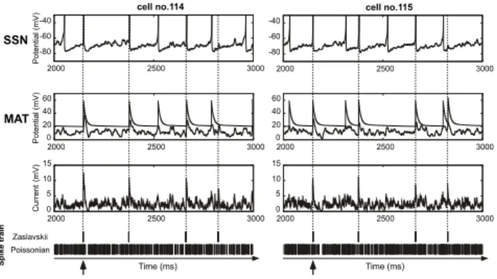
In the 1st layer we analyzed the effect of the model by comparing cells that received the same inputs. Figure 4 shows the example of two different neurons (cells no. 114 and 115) located in the 1st layer. In the bottom panel the in-put spike trains with dynamical information ratio D = 0.5 and the Poissonian background are sorted in order to emphasize the spikes belonging to Zaslavskii. Zaslavskii spikes increase the chance to overlap and to produce a stronger post-synaptic current by temporal summation with an increase in D. In this example, eight spikes belonging to the original Zaslavskii spike train arrive simultaneously at t = 2150 ms (see the upward arrow in the last panel of Fig. 4) and evoke a suprathreshold current that generates a spike.
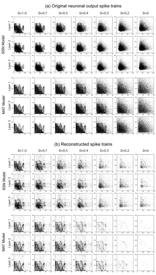
The return maps of the raw output spike trains of one representative neuron of each layer and for each neuronal model are shown in Fig. 5a as a function of D. As D decreased, the attractor contour become blurred. Notice that for exclusive Poissonian input spike trains (D = 0) the return maps of the SSN model (Fig. 5a (rightmost column) show a bias in the distribution of points, with empty bands
Table 1. Mean firing rate (spikes/s) of a neuron of SSN and MAT models as a function
of the order of the layer (1st-2nd-3rd) and of the dynamical information ratio D. SD ranged between 0.02 and 0.03 spikes/s.
SSN model MAT model
D 1 0.7 0.5 0.4 0.3 0.2 0 1 0.7 0.5 0.4 0.3 0.2 0
1st 6.4 6.1 5.9 5.7 5.4 5.1 4.8 6.6 6.4 6.1 5.7 5.3 4.9 4.5
2nd 6.8 6.6 6.4 6.2 5.8 5.4 5.0 7.7 7.1 6.7 6.4 5.8 5.2 4.5
Temporal information distributed across multiple spike trains 7 Time (ms) Time (ms) P o te n tia l( m V ) C u rr e n t (m V ) SSN Zaslavskii Poissonian 0 5 10 15 -80 -60 -40 0 20 40 60 MAT P o te n tia l( m V )
cell no.114 cell no.115
2000 2500 3000 2000 2500 3000 0 5 10 15 -80 -60 -40 0 20 40 60 2000 2500 3000 2000 2500 3000 2000 2500 3000 2000 2500 3000 S p ik e tr a in
Fig. 4. Left and right panels shows data from two neurons belonging to the 1st layer.
Dynamics of the membrane potentials for model SSN (first row) and for model MAT (second row), and the total post-synaptic input current (third row) are shown as a function of the input spike trains (bottom panels) where Zaslavskii and Poissonian spike trains are sorted out. The dynamical information ratio was set to D = 0.5.
near the axis, due to an internal temporal structure embedded within the model dynamics. In the MAT model it is interesting to observe that with an increase in the order of the layer the attractor contour become clearer even for D as low as D = 0.3. The “reconstructed spike trains” statistics are summarized in Table 2 and the return maps illustrated by Fig. 5b clearly show the noise filtering effect obtained by applying PGA, thus revealing the underlying attractor contour.
Table 2. Firing rate statistics of the reconstructed spike trains of SSN and MAT
neurons shown in Fig. 5b as a function of the order of the layer (1st-2nd-3rd) and of the dynamical information ratio D.
SSN model MAT model
D 1 0.7 0.5 0.4 0.3 0.2 0 1 0.7 0.5 0.4 0.3 0.2 0 Firing rate (spikes/s)
1st 5.2 3.9 2.7 2.1 1.6 1.2 1.1 5.0 5.1 3.4 1.8 1.1 0.3 0.2 2nd 5.0 4.1 3.3 2.7 2.4 1.8 1.3 5.2 5.2 4.6 3.4 1.4 0.3 0.2 3rd 4.8 4.1 3.0 2.9 2.0 1.7 1.5 5.2 5.2 4.8 3.7 1.8 0.8 0.1 Fano factor 1st 0.55 0.64 0.97 1.21 1.53 1.86 1.79 0.67 0.64 0.84 1.36 1.84 2.74 2.68 2nd 0.56 0.64 0.81 1.00 1.08 1.37 1.90 0.71 0.73 0.69 0.83 1.71 2.72 2.56 3rd 0.58 0.66 0.91 0.95 1.34 1.50 1.64 0.67 0.70 0.69 0.79 1.48 2.39 3.26 Similarity ratio (%) 1st 79.9 58.8 31.9 18.8 9.8 4.6 2.0 89.1 86.7 64.2 38.7 20.0 2.9 0.4 2nd 25.5 8.0 5.1 4.6 4.3 2.7 2.0 86.6 85.2 74.8 57.3 24.4 3.8 0.4 3rd 5.5 5.7 4.8 4.4 3.6 2.8 2.0 87.4 82.0 67.9 49.3 22.1 5.8 0.1
La ye r 1 La ye r 2 La ye r 3 D=1.0 D=0.7 D=0.5 D=0.4 D=0.3 D=0.2 D=0 La ye r 1 La ye r 2 La ye r 3 La ye r 1 La ye r 2 La ye r 3 La ye r 1 La ye r 2 La ye r 3
(a) Original neuronal output spike trains
D=1.0 D=0.7 D=0.5 D=0.4 D=0.3 D=0.2 D=0
(b) Reconstructed spike trains
S S N M od el M A T M od el M A T M od el S S N M od el
Fig. 5. Return maps of neuronal output spike trains and spike trains reconstructed from
them. One neuron from each layer was selected as an example for several dynamical information ratio D and for both of the SSN and MAT models.
Temporal information distributed across multiple spike trains 9 With a decrease of D, the number of spikes detected by PGA decreased (i.e. the firing rate of the reconstructed spike trains decreased). In the case of
SSN significant amount of spikes were detected by PGA even for D≤ 0.3, but
the return maps don’t show the contour of the Zaslavskii attractor and the preferred firing sequences detected by PGA can be attributed to the intrinsic dynamics of the model. On the opposite, the MAT model seldom introduced a temporal structure in the output spike train due to intrinsic model dynamics. With the MAT model notice that the similarity ratio and the firing rate of the reconstructed spike train increased from the 1st to the higher order layers with D = 0.4. In both models, the Fano factor was larger for small values of D and
became less than 1 at the third layer for both models with D ≥ 0.4. Looking
at the similarity ratio the two models behaved very differently. Furthermore, for the MAT model only the similarity ratio tended to be preserved across the layers
for D≥ 0.5 and was even near 0.5 in the 3rd layer with d = 0.4.
4
Discussion
The deterministic sequence of spikes generated by a chaotic attractor was dis-tributed and embedded in the input spike trains fed to a partially conver-gent/divergent feed-forward layered network. We have provided evidence that a multiple-timescale adaptive threshold (MAT) neuronal model [9] was able to retain and transmit a sizable amount of the initial temporal information up to the 3rd layer with dynamical information ratio as low as D = 0.4. Conversely, a simple spiking neuron (SSN) model [8] introduced a bias in the temporal pattern of the output spike train associated to its model dynamics which interfered with the input temporally organized information. It is interesting to notice that by passing through the successive layers, the similarity ratio of the SSN neurons decreased drastically despite the fact the reconstructed spike train and the Fano factor were kept rather high.
The current study does not pretend to exclude SSN models from being able to preserve and transmit temporal information through complex neural network circuits because we did not carry out a parameter search of that class of models in order to optimize the performance. The MAT model is interesting because in presence of a pure stochastic input very few spikes were detected by the PGA filtering procedure, thus indicating that this model did not introduce a bias. We consider that this work may be viewed as seminal addressing the novel problem because it suggests that MAT class of models might represent a good candidate for integrating a distributed deterministic temporal information and preserve its dynamics through networks of cell assemblies. Our further work is aimed to determine the limits of this performance by increasing the number of layers, designing inhomogeneous and diverging/converging networks with recur-rent connections and with the introduction of explicit synaptic delays and spike timing dependent plasticity.
Acknowledgments
This study was partially funded by the bi-national JSPS/INSERM grant SYR-NAN and Japan-France Research Cooperative Program.
References
1. Mpitsos, G.J.: Chaos in brain function and the problem of nonstationarity: a
commentary. In Basar, E., Bullock, T.H., eds.: Dynamics of sensory and cognitive processing by the brain. Springer-Verlag (1989) 521–535
2. Celletti, A., Villa, A.E.P.: Determination of chaotic attractors in the rat brain. J. Stat. Physics 84 (1996) 1379–1385
3. Tetko, I.V., Villa, A.E.: A comparative study of pattern detection algorithm and dynamical system approach using simulated spike trains. Lecture Notes in Com-puter Science 1327 (1997) 37–42
4. Asai, Y., Yokoi, T., Villa, A.E.P.: Detection of a dynamical system attractor from spike train analysis. Lecture Notes in Computer Sciences 4131 (2006) 623–631
5. Asai, Y., Guha, A., Villa, A.E.P.: Deterministic neural dynamics transmitted
through neural networks. Neural Networks 21 (2008) 799–809 6. Abeles, M.: Local Cortical Circuits. Springer Verlag (1982)
7. Asai, Y., Villa, A.E.: Spatio temporal filtering of the distributed spike train with deterministic structure by ensemble of spiking neurons. In: The 8th Intenational Neural Coding Workshop Proceedings, Tainan, Taiwan (2009) 81–83
8. Izhikevich, E.M.: Which model to use for cortical spiking neurons? IEEE Trans-actions on Neural Networks 15 (2004) 1063–1070
9. Kobayashi, R., Tsubo, Y., Shinomoto, S.: Made-to-order spiking neuron model equipped with a multi-timescale adaptive threshold. Front Comput Neurosci 3 (2009) doi:10.3389/neuro.10.009.2009
10. Brette, R., Gerstner, W.: Adaptive exponential integrate-and-fire model as an effective description of neuronal activity. J. Neurophysiol. 94 (2005) 3637–3642 11. Zaslavskii, G.M.: The simplest case of a strange attractor. Phys. Let. 69A (1978)
145–147
12. Villa, A.E.P., Tetko, I.V.: Spatiotemporal activity patterns detected from single cell measurements from behaving animals. Proceedings SPIE 3728 (1999) 20–34 13. Tetko, I.V., Villa, A.E.P.: A pattern grouping algorithm for analysis of
spatiotem-poral patterns in neuronal spike trains. 1. detection of repeated patterns. J. Neu-rosci. Meth. 105 (2001) 1–14
14. Abeles, M., Gat, I.: Detecting precise firing sequences in experimental data. Journal of Neuroscience Methods 107 (2001) 141–154
15. Sacerdote, L., Villa, A.E., Zucca, C.: On the classification of experimental data modeled via a stochastic leaky integrate and fire model through boundary values. Bull. Math. Biol. 68 (2006) 1257–1274