Constructing Symbolic Representations for High-Level Planning
The MIT Faculty has made this article openly available.
Please share
how this access benefits you. Your story matters.
Citation
Konidaris, George, Leslie Pack Kaelbling, and Tomas Lozano-Perez.
"Constructing Symbolic Representations for High-Level Planning."
28th AAAI Conference on Artificial Intelligence (July 2014).
As Published
http://www.aaai.org/ocs/index.php/AAAI/AAAI14/paper/view/8424
Publisher
Association for the Advancement of Artificial Intelligence (AAAI)
Version
Author's final manuscript
Citable link
http://hdl.handle.net/1721.1/100720
Terms of Use
Creative Commons Attribution-Noncommercial-Share Alike
Constructing Symbolic Representations for High-Level Planning
George Konidaris, Leslie Pack Kaelbling and Tomas Lozano-Perez
MIT Computer Science and Artificial Intelligence Laboratory 32 Vassar Street, Cambridge MA 02139 USA
{gdk, lpk, tlp}@csail.mit.edu
Abstract
We consider the problem of constructing a symbolic description of a continuous, low-level environment for use in planning. We show that symbols that can repre-sent the preconditions and effects of an agent’s actions are both necessary and sufficient for high-level plan-ning. This eliminates the symbol design problem when a representation must be constructed in advance, and in principle enables an agent to autonomously learn its own symbolic representations. The resulting representa-tion can be converted into PDDL, a canonical high-level planning representation that enables very fast planning.
Introduction
A core challenge of artificial intelligence is creating intelli-gent aintelli-gents that can perform high-level learning and plan-ning, while ultimately performing control using low-level sensors and actuators. Hierarchical reinforcement learning approaches (Barto and Mahadevan 2003) attempt to ad-dress this problem by providing a framework for learning and planning using temporally abstract high-level actions. One motivation behind such approaches is that an agent that has learned a set of high-level actions should be able to plan using them to quickly solve new problems, without further learning. However, planning directly in such high-dimensional, continuous state spaces remains difficult.
By contrast, high-level planning techniques (Ghallab, Nau, and Traverso 2004) are able to solve very large prob-lems in reasonable time. These techniques perform planning using pre-specified symbolic state descriptors, and opera-tors that describe the effects of actions on those descrip-tors. Although these methods are usually used for planning in discrete state spaces, they have been combined with low-level motion planners or closed-loop controllers to construct robot systems that combine high-level planning with low-level control (Nilsson 1984; Malcolm and Smithers 1990; Cambon, Alami, and Gravot 2009; Choi and Amir 2009; Dornhege et al. 2009; Wolfe, Marthi, and Russell 2010; Kaelbling and Lozano-P´erez 2011). Here, a symbolic state at the high level refers to (and abstracts over) an infinite set of low-level states. However, in all of these cases the robot’s symbolic representation was specified by its designers.
Copyright c 2014, Association for the Advancement of Artificial
Intelligence (www.aaai.org). All rights reserved.
We consider the problem of constructing a symbolic rep-resentation suitable for evaluating plans composed of se-quences of actions in a continuous, low-level environment. We can create such a representation by reasoning about po-tential propositional symbols via the sets of states they ref-erence. We show that propositional symbols describing low-level representations of the preconditions and effects of each action are both sufficient and necessary for high-level plan-ning, and discuss two classes of actions for which the ap-propriate symbols can be concisely described. We show that these representations can be used as a symbol algebra suit-able for high-level planning, and describe a method for con-verting the resulting representation into PDDL (McDermott et al. 1998), a canonical high-level planning representation.
Our primary contribution is establishing a close relation-ship between an agent’s actions and the symbols required to plan to use them: the agent’s environment and actions com-pletely determine the symbolic representation required for planning. This removes a critical design problem when con-structing agents that combine high-level planning with low-level control; moreover, it in principle enables an agent to construct its own symbolic representation through learning.
Background and Setting
Semi-Markov Decision Processes
We assume that the low-level sensor and actuator space of the agent can be described as a fully observable, continuous-state semi-Markov decision process (SMDP), described by a tuple M = (S, O, R, P, γ), where S ⊆ Rn is the n-dimensional continuous state space; O(s) returns a finite set of temporally extended actions, or options (Sutton, Pre-cup, and Singh 1999), available in state s ∈ S; R(s0, t|s, o) is the reward received when executing action o ∈ O(s) at state s ∈ S, and arriving in state s0 ∈ S after t time steps; P (s0, t|s, o) is a PDF describing the probability of arriving in state s0 ∈ S, t time steps after executing action o ∈ O(s) in state s ∈ S; and γ ∈ (0, 1] is a discount factor.
An option o consists of three components: an option pol-icy, πo, which is executed when the option is invoked; an initiation set, Io= {s|o ∈ O(s)}, which describes the states in which the option may be executed; and a termination con-dition, βo(s) → [0, 1], which describes the probability that an option will terminate upon reaching state s. The
combi-nation of reward model, R(s0, t|s, o), and transition model, P (s0, t|s, o), for an option o is known as an option model.
An agent that possesses option models for all of its op-tions is capable of sample-based planning (Sutton, Precup, and Singh 1999; Kocsis and Szepesv´ari 2006), although do-ing so in large, continuous state spaces is very difficult.
High-Level Planning
High-level planning operates using symbolic states and op-erators. The simplest formalism is the set-theoretic repre-sentation(Ghallab, Nau, and Traverso 2004). Here, a plan-ning domain is described by a set of propositions P = {p1, ..., pn} and a set of operators A = {α1, ..., αm}. In a continuous problem, each proposition holds in an infinite number of low-level states; a high-level state is obtained by assigning a truth value to every pi ∈ P.
Each operator αi is described by a tuple αi = (precondi, effect
+ i , effect
−
i ), where precondi ⊆ P lists all propositions that must be true in a state for the operator to be applicable at that state, and positive and negative effects, effect+i ⊆ P and effect−i ⊆ P, list the propositions set to true or false, respectively, as a result of applying the oper-ator. All other propositions retain their values. A planning problem is obtained by augmenting the domain description with a start state, s0, and a set of goal states, Sg.
A more common formulation is the classical representa-tion(Ghallab, Nau, and Traverso 2004), which uses a rela-tional representation to more compactly describe the plan-ning domain. For simplicity, we adopt the set-theoretic rep-resentation and leave parametrizing it to future work.
Problems in both formulations are typically described us-ing the Plannus-ing and Domain Definition Language or PDDL (McDermott et al. 1998), which serves as the input format for most general-purpose planners. Although such methods have been widely applied—even in continuous problems— with few exceptions the set of propositions and their seman-tics must be supplied by a human designer.
Symbols and Plans
Given an SMDP, our goal is to build an abstract representa-tion of the task for use in high-level planning. In this secrepresenta-tion we define a propositional symbol as a test that is true in some set of states. We then define a plan as a sequence of option executions from a set of start states, and the plan space as the set of all possible plans. This allows us to reason about the symbols required to evaluate the feasibility of any plan in the plan space. We begin with a working definition of the notion of a symbol:
Definition 1. A propositional symbol σZ is the name asso-ciated with a test τZ, and the corresponding set of states Z = {s ∈ S | τZ(s) = 1}.
Symbol σZis a name for a proposition, specified by both a test (or classifier) τZdefined over the state space, and an as-sociated set Z ⊆ S for which the test returns true. The set of states Z is referred to as the symbol’s grounding, and spec-ifies the symbol’s semantics. A symbol’s grounding can be represented in two different ways: an extensional represen-tationthat lists the states in which the proposition holds—
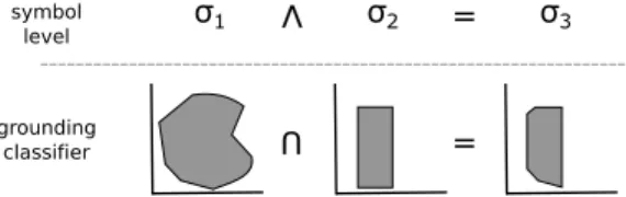
impossible in our case, since our low-level state space is continuous—and an intensional representation, a classifier that determines membership in that set of states. The classi-fier allows us to express the set of states compactly, and also to learn a representation of them (if necessary). These rep-resentations both refer to the same set of states (and there-fore are in some sense equivalent) but we can perform task-based planning by manipulating and reasoning about inten-sional grounding representations—we compute the results of logical operations on symbols by computing the resulting grounded classifier. This process is depicted in Figure 1.
σ3 σ2 σ1 V = = U symbol level grounding classifier
Figure 1: A logical operation on two symbols, along with the corresponding grounding sets.
We therefore require the grounding classifiers to support the ability to efficiently compute the following operations: 1) the union of two classifiers (equivalently, the or of two symbols); 2) the intersection of two classifiers (equivalently, the and of two symbols); 3) the complement of a classi-fier (equivalently, the not of a symbol); 4) whether or not a classifier refers to the empty set. (This allows us evalu-ate the subset operator: A ⊆ B iff ¬A ∩ B is empty; con-sequently, we can test implication.) The first three of these operations take classifiers as inputs and return a classifier representing the result of a logical operation. This defines a symbol algebra (a concrete boolean algebra) that allows us to construct classifiers representing the results of boolean operations applied to our symbols. Classifiers that support these operations include, for example, decision trees (which we use throughout this paper for ease of visualization) and boolean ensembles of linear classifiers.
We next define the plan space of a domain. For simplicity, we aim to find a sequence of actions guaranteed to reach a goal state, without reference to cost.
Definition 2. A plan p = {o1, ..., opn} from a state set
Z ⊆ S is a sequence of options oi ∈ O, 1 ≤ i ≤ pn, to be executed from some state in Z. A plan is feasible when the probability of being able to execute it is 1, i.e., @S = {s¯ 1, ..., sj} such that s1 ∈ Z, oi ∈ O(si) and P (si+1|si, oi) > 0, ∀i < j, and oj∈ O(s/ j) for any j < pn. Definition 3. The plan space for an SMDP is the set of all tuples (Z, p), where Z ⊆ S is a set of states (equivalently, a start symbol) in the SMDP, and p is a plan.
For convenience, we treat the agent’s goal set g—itself a propositional symbol—as an option og with Ig = g, βg(s) = 1, ∀s, and a null policy.
Definition 4. A plan tuple is satisficing for goal g if it is feasible, and its final action is goal optionog.
The role of a symbolic representation is to determine whether any given plan tuple (Z, p) is satisficing for goal
g, which we can achieve by testing whether it is feasible (since then determining whether it is satisficing follows triv-ially). In the following section, we define a set of proposi-tional symbols (via their groundings) and show that they are sufficient to test feasibility in any SMDP.
Symbols for Propositional Planning
To test the feasibility of a plan, we begin with a set of possi-ble start states, and repeatedly compute the set of states that can be reached by each option, checking in turn that the re-sulting set is a subset of the initiation set of the following option. We must therefore construct abstract representations for the initiation set of each option, and that enable us to compute the set of states an agent may find itself in as a result of executing an option from some start set of states. We begin by defining a class of symbols that represent the initiation set of an option:
Definition 5. The precondition of option o is the symbol re-ferring to its initiation set: Pre(o) = σIo.
We now define a symbolic operator that computes the con-sequences of taking an action in a set of states:
Definition 6. Given an option o and a set of states X ⊆ S, we define the image ofo from X as: Im(X, o) = {s0|∃s ∈ X, P (s0|s, o) > 0}.
The image operator Im(X, o) computes the set of states that might result from executing o from some state in X. Theorem 1. Given an SMDP, the ability to represent the preconditions of each option and to compute the image op-erator is sufficient for determining whether any plan tuple (Z, p) is feasible.
Proof. Consider an arbitrary plan tuple (Z, p), with plan length n. We set z0 = Z and repeatedly compute zj+1 = Im(zj, pj), for j ∈ {1, ..., n}. The plan tuple is feasible iff zi⊆ Pre(pi+1), ∀i ∈ {0, ..., n − 1}.
Since the feasibility test in the above proof is bicondi-tional, any other feasibility test must express exactly those conditions for each pair of successive options in a plan. In some SMDPs, we may be able to execute a different test that evaluates to the same value everywhere (e.g., if every option flips a set of bits indicating which options can be run next), but we can employ an adversarial argument to construct an SMDP in which any other test is incorrect. Representing the image operator and precondition sets are therefore also nec-essary for abstract planning. We call the symbols required to name an option’s initiation set and express its image opera-tor that option’s characterizing symbols.
The ability to perform symbolic planning thus hinges on the ability to symbolically represent the image operator. However, doing this for an arbitrary option can be arbitrar-ily hard. Consider an option that maps each state in its ini-tiation set to a single (but arbitrary and unique) state in S. In this case we can do no better than expressing Im(Z, o) as a union of uncountably infinitely many singleton symbols. Fortunately, however, we can concisely represent the image operator for at least two classes of options in common use.
Subgoal Options
One common type of option—especially prevalent in re-search on skill discovery methods—is the subgoal option (Precup 2000). Such an option reaches a set of states (re-ferred to as its subgoal) before terminating, and the state it terminates in can be considered independent of the state from which it is executed. This results in a particularly sim-ple way to express the image operator.
Definition 7. The effect set of subgoal option o is the sym-bol representing the set of all states that an agent can pos-sibly find itself in after executing o: Eff(o) = {s0|∃s ∈ S, t, P (s0, t|s, o) > 0}.
For a subgoal option, Im(Z, o) = Eff(o), ∀Z ⊆ S. This is a strong condition, but we may in practice be able to treat many options as subgoal options even when they do not strictly meet it. This greatly simplifies our representational requirements at the cost of artificially enlarging the image (which is a subset of Eff(o) for any given starting set).
A common generalization of a subgoal option is the par-titioned subgoal option. Here, the option’s initiation set can be partitioned into two or more subsets, such that the option behaves as a subgoal option from each subset. For example, an option that we might describe as walk through the door you are facing; if there are a small number of such doors, then the agent can be considered to execute a separate sub-goal option when standing in front of each. In such cases, we must explicitly represent each partition of the initiation set separately; the image operator is then the union of the effect sets of each applicable partitioned option.
Unfortunately, subgoal options severely restrict the poten-tial goals an agent may plan for: all feasible goals must be a superset of one of the effect sets. However, they do lead to a particularly simple planning mechanism. Since a subset test between the precondition of one option and the effects set of another is the only type of expression that need ever be evaluated, we can test all such subsets in time O(n2) for O(n) characterizing sets, and build a directed plan graph G with a vertex for each characterizing set, and an edge present between vertices i and j iff Eff(oi) ⊆ Pre(oj). A plan tuple (p, Z) where p = {o1, ..., opn} is feasible iff Z ⊆ Io1 and a
path from o1to opnexists in G.
For an option to be useful in a plan graph, its effects set should form a subset of the initiation set of any op-tions the agent may wish to execute after it. The opop-tions should therefore ideally have been constructed so that their termination conditions lie inside the initiation sets for po-tential successor options. This is the principle underlying pre-image backchaining (Lozano-Perez, Mason, and Taylor 1984; Burridge, Rizzi, and Koditschek 1999), the LQR-Tree (Tedrake 2009) feedback motion planner, and the skill chain-ing (Konidaris and Barto 2009b) skill acquisition method.
Abstract Subgoal Options
A more general type of option—implicitly assumed by all STRIPS-style planners—is the abstract subgoal option, where execution sets some of the variables in the low-level state vector to a particular set of values, and leaves others unchanged. (As above, we may generalize abstract subgoal
options to partitioned abstract subgoal options.) The sub-goal is said to be abstract because it is satisfied for any value of the unchanged variables. For example, an option to grasp an object might terminate when that grasp is achieved; the room the robot is in and the position of its other hand are irrelevant and unaffected.
Without loss of generality, we can write the low-level state vector s ∈ S given o as s = [a, b], where a is the part of the vector that changes when executing o (o’s mask), and b is the remainder. We now define the following operator:
Definition 8. Given an option o and a set of states Z ⊆ S, we define the projection of Z with respect to o (denoted Project(Z, o)) as: Project(Z, o) = {[a, b]|∃a0, [a0, b] ∈ Z}.
Projection expands the set of states named by Z by re-moving the restrictions on the value of the changeable por-tion of the state descriptor. This operator cannot be ex-pressed using set operations, and must instead be obtained by directly altering the relevant classifier.
x y Z x y Eff(o) Abstract Subgoal Project(Z,o) Im(Z,o)
Figure 2: Im(Z, o) for abstract subgoal option o can be ex-pressed as the intersection of the projection operator and o’s effects set. Here, o has a subgoal in x, leaving y unchanged. The image operator for an abstract subgoal option can be computed as Im(Z, o) = Project(Z, o) ∩ Eff(o) (see Figure 2). We can thus plan using only the precondition and effects symbols for each option.
Constructing a PDDL Domain Description
So far we have described a system where planning is per-formed using symbol algebra operations over grounding classifiers. We may wish to go even further, and construct a symbolic representation that allows us to plan without ref-erence to any grounding representations at all.
A reasonable target is converting a symbol algebra into a set-theoretic domain specification expressed using PDDL. This results in a once-off conversion cost, after which the complexity of planning is no worse than ordinary high-level planning, and is independent of the low-level SMDP.
A set-theoretic domain specification uses a set of propo-sitional symbols P = {p1, ..., pn} (each with an associated grounding classifier G(pi)), and a state Ptis obtained by as-signing a truth value Pt(i) to every pi ∈ P. Each state Pt must map to some grounded set of states; we denote that set of states by G(Pt). A scheme for representing the domain using STRIPS-like operators and propositions must commit to a method for determining the grounding for any given Pt so that we can reason about the correctness of symbolic con-structions, even though that grounding is never used during
planning. We use the following grounding scheme: G(Pt) = ∩i∈IG(pi), I = {i|Pt(i) = 1}.
The grounding classifier of state Ptis the intersection of the grounding classifiers corresponding to the propositions true in that state. One can consider the propositions set to true as “on”, in the sense that they are included in the grounding intersection, and those set to false as “off”, and not included. The key property of a deterministic high-level domain de-scription is that the operator dede-scriptions and propositional symbols are sufficient for planning—we can perform plan-ning using only the truth value of the propositional sym-bols, without reference to their grounding classifiers. This requires us to determine whether or not an option oican be executed at Pt, and if so to determine a successor state Pt+1, solely by examining the elements of Pt.
Our method is based on the properties of abstract subgoal options: that only a subset of state variables are affected by executing each option; that the resulting effects set is inter-sected with the previous set of states after the those variables have been projected out; and that the remaining state vari-ables are unaffected. Broadly, we identify a set of factors— non-overlapping sets of low-level variables that could be changed simultaneously by an option execution—and then use the option effects sets to generate a set of symbols corre-sponding to any reachable grounding of each set of factors. Finally, we use this set of symbols to produce an operator description for each option.
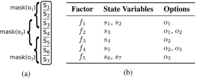
Defining Factors Given a low-level state representation s = [s1, ..., sn], we define a mapping from each low-level state variable to the set of options capable of changing its value: modifies(si) = {oj|i ∈ mask(oj), oj ∈ O}. We next partition s into factors, f1, ..., fm, each of which is a set of state variables that maps to the same unique set of options. An example of this process is shown in Figure 3.
{
{
{
mask(o1) mask(o2) mask(o3) s3 s2 s4 s6 s1 s5 s7 (a)Factor State Variables Options
f1 s1, s2 o1 f2 s3 o1, o2 f3 s4 o2 f4 s5 o2, o3 f5 s6, s7 o3 (b)
Figure 3: An example 7-variable low-level state vector, with three option masks (a). This is partitioned into 5 factors (b). We denote the set of options modifying the variables in factor fias options(fi), and similarly the set of factors con-taining state variables that are modified by option oj as factors(oj). In a slight abuse of notation, we also denote the factors containing variables used in the grounding classifier for symbol σkas factors(σk).
Building the Symbol Set Executing option oiprojects the factors it changes out of the current state descriptor, which is then intersected with its effect set Eff(oi). Future execution of any option oj where factors(oi) ∩ factors(oj) 6= ∅ will
project the overlapping factors out of Eff(oi). We therefore require a propositional symbol for each option effects set with all combinations of factors projected out. However, we can represent the effect of projecting out a factor compactly if it obeys the following independence property:
Definition 9. Factor fsis independent in effect set Eff(oi) iff Eff(oi)= Project(Eff(oi), fs) ∩ Project(Eff(oi), factors(oi)\ fs).
If fs is independent in Eff(oi), we can break Eff(oi) into the two components Project(Eff(oi), fs) and Project(Eff(oi), factors(oi) \ fs) and create a separate proposition for each. We repeat this for each independent factor, each time using the more general effect set we obtain by projecting out previous independent factors.
Let Effr(oi) denote the effect set that remains after projecting out all independent factors from Eff(oi), and factorsr(oi) denote the remaining factors. We will require a separate proposition for Effr(oi) with each possible subset of factorsr(oi) projected out. Therefore, we construct a vo-cabulary P containing the following propositional symbols: 1. For each option oi and factor fsindependent in Eff(oi),
create a symbol for Project(Eff(oi), factors(oi) \ fs). 2. For each set of factors fr⊆ factorsr(oi), create a symbol
for Project(Effr(oi), fr).
We discard duplicate propositions (which have the same grounding set as an existing proposition), and propositions which correspond to the entire state space (as these have no effect on the grounding intersection). We now show that these symbols are sufficient for symbolically describing a problem by using them to construct a sound operator de-scription for each option.
Constructing Operator Descriptions Executing operator oiresults in the following effects:
1. All symbols for each component of Eff(oi) that depends on a factor independent in Eff(oi), and an additional sym-bol for Effr(oi) if necessary, are set to true.
2. All symbols σj ⊆ Pre(oi) such that factors(σj) ⊆ factors(oi) are set to false.
3. All currently true symbols σj ⊆ Pre(oi), where fij = factors(σj) ∩ factors(oi) 6= ∅ but factors(σj) 6⊆ factors(oi), are set to false. For each such σj, the symbol Project(σj, fij) is set to true.
Recall that we compute the image of an abstract subgoal option oifrom an existing set of states Z using the equation Im(Z, oi) = Project(Z, oi) ∩ Eff(oi). The first effect in the above list corresponds to the second component of the im-age equation, and can be considered the primary effect of the option. The remaining two types of effects model the pro-jection component of the image equation. The second type of effects removes propositions defined entirely using vari-ables within mask(oi), and whose effects are thus eliminated by the projection operator. The third effects type models the side-effects of the option, where an existing classifier has the variables affected by the projection (those in mask(oi)) projected out. This is depicted in Figure 4.
option effect pr opositions pr opositions tru e at t ime t f3 f2 f4 f6 f1 f5 f7
{
{
{
{
{
σ4 σ5 σ3 σ2 σ1At time t, the following symbols are true:
σ1, σ2, and σ3.
After executing the option, the following symbols are true:
σ3, σ4, σ5, and σ6,
where σ6 = Proj(σ1, f2). σ1and
σ2are no longer true.
Figure 4: An example effect computation. At time t, σ1, σ2, and σ3are true. The option’s effect set is represented by σ4 and independent factor σ5. After execution, σ3remains true because its factors lie outside of the option mask, while σ2 is set to false because its factors are covered by the mask. The factors used by σ1 are only partially covered, so it is set to false and σ6 = Proj(σ1, f2) is set to true. σ4and σ5 correspond go the option’s direct effects and are set to true.
Theorem 2. Given abstract state descriptor Pt, optionoj such thatG(Pt) ⊆ Pre(oj), andPt+1as computed above:
G(Pt+1) = Im(G(Pt), oj). Proof. Recall our grounding semantics:
G(Pt) = ∩i∈IG(pi), I = {i|Pt(i) = 1}, and the definition of the image operator:
Im(G(Pt), oj) = Project(G(Pt), oj) ∩ Eff(oj). Substituting, we see that:
Im(G(Pt), oj) = Project(∩i∈IG(pi), oj) ∩ Eff(oj) = ∩i∈IProject(G(pi), oj) ∩ Eff(oj). We can split I into three sets: Iu, which contains indices for symbols whose factors do not overlap with oj; Ir, which contains symbols whose factors are a subset of mask(oj); and Io, the remaining symbols whose factors overlap. Pro-jecting out mask(oj) leaves the symbols in Iu unchanged, and replaces those in Irwith the universal set, so:
Im(G(Pt), oj) = ∩i∈IuG(pi) ∩i∈IoProject(G(pi), oj) ∩ Eff(oj).
For each i ∈ Io, we can by construction find a k such that G(pk) = Project(G(pi), oj). Let K be the set of such in-dices. Then we can write:
Im(G(Pt), oj) = ∩i∈IuG(pi) ∩k∈KG(pk) ∩ Eff(oj).
The first term on the right hand side of the above equality corresponds to the propositions left alone by the operator ap-plication; the second term to the third type of effects propo-sitions; the third term to the first type of effects propopropo-sitions; and Irto the second type of (removed) effects propositions. These are exactly the effects enumerated by our operator model, so Im(G(Pt), oj) = G(Pt+1).
Finally, we must compute the operator preconditions, which express the conditions under which the option can be executed. To do so, we consider the preimage Pre(oi)
for each option oi, and the factors is is defined over, factors(Pre(oi)). Our operator effects model ensures that no two symbols defined over the same factor can be true simul-taneously. We can therefore enumerate all possible “assign-ments” of factors to symbols, compute the resulting ground-ing classifier, and determine whether it is a subset of Pre(oi). If so, the option can be executed, and we can output an op-erator description with the appropriate preconditions and ef-fects. We omit the proof that the generated preconditions are correct, since it follows directly from the definition.
Note that the third type of effects (expressing the op-tion’s side effects) depends on propositions other than those used to evaluate the option’s preimage. We can express these cases either by creating a separate operator description for each possible assignment of relevant propositions, or more compactly via PDDL’s support for conditional effects.
Since the procedure for constructing operator descrip-tions given in this section uses only proposidescrip-tions enumerated above, it follows that P is sufficient for describing the sys-tem. It also follows that the number of reachable symbols in a symbol algebra based on abstract subgoal options is finite. Computing the factors requires time in O(n|F ||O|), where F , the set of factors, has at most n elements (where n is the dimension of the original low-level state space). Enumerating the symbol set requires time in O(|O||F |c) for the independent factors and O(|O|2|F |c) for the depen-dent factors in the worst case, where each symbol alge-bra operation is O(c). This results in a symbol set of size |P| = O(FI+ 2FD), where FI indicates the number of sym-bols resulting from independent factors, and FDthe number of factors referred to by dependent effects sets. Computing the operator effects is in time O(|P||O|), and the precondi-tions in time O(|O||P||F |) in the worst case.
Although the resulting algorithm will output a correct PDDL model for any symbol algebra with abstract sub-goals, it has a potentially disastrous worst-case complexity, and the resulting model can be exponentially larger than the O(|O|) source symbol algebra. We expect that conversion will be most useful in problems where the number of factors is small compared to the number of original state variables (|F | n), most or all of the effects sets are independent in all factors (FD FI), many symbols repeat (small |P|), and most precondition computations either fail early or suc-ceed with a small number of factors. These properties are typically necessary for a domain to have a compact PDDL model in general.
Planning in the Continuous Playroom
In the continuous playroom domain (Konidaris and Barto 2009a), an agent with three effectors (an eye, a hand, and a marker) is placed in a room with five objects (a light switch, a bell, a ball, and red and green buttons) and a monkey; the room also has a light (initially off) and music (also initially off). The agent is given options that allow it to move a spec-ified effector over a specspec-ified object (always executable, re-sulting in the effector coming to rest uniformly at random within 0.05 units of the object in either direction), plus an “interact” option for each object (for a total of 20 options).
The effectors and objects are arranged randomly at the start of every episode; one arrangement is depicted in Figure 5.
Figure 5: An instance of the continuous playroom domain. Interacting with the buttons or the bell requires the light to be on, and the agent’s hand and eye to be placed over (within 0.05 units in either direction) the relevant object. The ball and the light switch are brightly colored and can be seen in the dark, so they do not require the light to be on. Interacting with the green button turns the music on; the red button turns it off. Interacting with the light switch turns the lights on or off. Finally, if the agent’s marker is on the bell and it inter-acts with the ball, the ball is thrown at the bell and makes a noise. If this happens when the lights are off and the music is on, the monkey cries out, and the episode ends. The agent’s state representation consists of 33 continuous state variables describing the x and y distance between each effector and each object, the light level (0 when the light is off, and drop-ping off from 1 with the squared distance from the center of the room when the light is on), the music volume (selected at random from the range [0.3, 1.0] when the green button is pressed), and whether the monkey has cried out.
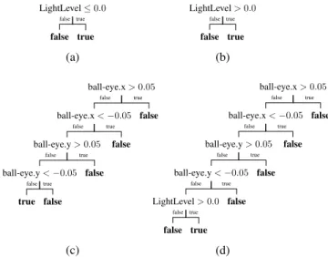
We first construct the appropriate symbolic descriptions for the continuous playroom by hand, following the theory developed above. First, we partition the option initiation sets to obtain partitioned abstract subgoal options; we then con-struct models of the relevant masks and effects sets. For ex-ample, Figure 6 shows the two characterizing sets for mov-ing the eye over the ball. The light level perceived by the agent changes with eye movement if the light is on and re-mains unchanged if it is not, so we partition the initiation set based on the existing light level.
Converting these symbolic descriptions to PDDL was completed in approximately 0.4 seconds. This resulted in 6 factors, three containing variables describing the distance between an effector and all of the objects, and one each for the music, the lights, and the monkey’s cry. The factors and the symbol algebra operator descriptors generated 20 unique symbol groundings—all effects sets resulted in independent factor assignments. An example operator description with its symbol groundings is shown in Figure 7.
We tested planning on three goals, each starting from the set of all states where the monkey is not crying out and the lights and music are off. We implemented a breadth-first symbol algebra planner in Java, and also used the au-tomatically generated PDDL description as input to the FF planner (Hoffmann and Nebel 2001). Timing results, given in Table 1, show that both systems can solve the resulting search problem very quickly, though FF (a modern heuristic
LightLevel ≤ 0.0 true false false true (a) LightLevel > 0.0 true false false true (b) ball-eye.x > 0.05 false ball-eye.x < −0.05 false ball-eye.y > 0.05 false ball-eye.y < −0.05 false true false true false true false true false true (c) ball-eye.x > 0.05 false ball-eye.x < −0.05 false ball-eye.y > 0.05 false ball-eye.y < −0.05 false LightLevel > 0.0 true false false true false true false true false true false true (d)
Figure 6: The two characterizing sets of the option for mov-ing the eye over the ball. The precondition classifier of the first characterizing set (a) includes states where the light is off. Its effect mask does not include LightLevel, and its effects set (c) indicates that the relationship between the eye and the ball is set to a specific range. The precondi-tion classifier for the second characterizing set (b) includes only states where the light is on. Its effects mask includes the LightLevel variable, which its effect set (d) indicates could change to any positive value after option execution, as the position of the eye affects the amount of light received.
planner) can solve it roughly a thousand times faster than a naive planner using a symbol algebra. The resulting plans are guaranteed to reach the goal for any domain configura-tion where the start symbol holds. We know of no existing sample-based SMDP planner with similar guarantees.
Symbol Algebra (BFS) PDDL (FF)
Goal Depth Visited Time (s) Visited Time (s)
Lights On 3 199 1.35 4 0.00199 Music On 6 362 2.12 9 0.00230 Monkey Cry 13 667 3.15 30 0.00277
Table 1: The time required, and number of nodes visited, for the example planning problems. Results were obtained on a 2.5Ghz Intel Core i5 processor and 8GB of RAM.
To demonstrate symbol acquisition from experience, we gathered 5, 000 positive and negative examples1of each op-tion’s precondition and effects set by repeatedly creating a new instance of the playroom domain, determine which op-tions could be executed at each state, and then sequentially executing options at random. For the effects set, we used option termination states as positive examples and states en-countered during option execution but before termination as negative examples. We used the WEKA toolkit (Hall et al.
1
This number was chosen arbitrarily and does not reflect the difficulty of learning the relevant sets.
(:action interact_greenbutton :parameters ()
:precondition (and (symbol1) (symbol2) (symbol3)) :effect (and (symbol17)
(not (symbol18))))
(a) Generated Operator
LightLevel > 0.0 LightLevel ≤ 1.0 true false false true false false true (b) symbol1 greenbutton-eye.x ≥ −0.05 greenbutton-eye.x ≤ 0.05 greenbutton-eye.y ≥ −0.05 greenbutton-eye.y ≤ 0.05 true false false true false false true false false true false false true (c) symbol2 greenbutton-hand.x ≥ −0.05 greenbutton-hand.x ≤ 0.05 greenbutton-hand.y ≥ −0.05 greenbutton-hand.y ≤ 0.05 true false false true false false true false false true false false true (d) symbol3 MusicLevel ≥ 0.3 MusicLevel ≤ 1.0 true false false true false false true (e) symbol17 MusicLevel = 0.0 true false false true (f) symbol18
Figure 7: The automatically generated PDDL descriptor for interacting with the green button (a) with the groundings of the automatically generated symbols it mentions (b–f). The operator symbolically expresses the precondition that the light is on and the hand and eye are over the green but-ton, and that, as a result of executing the operator, the music is on, and the music is no longer off.
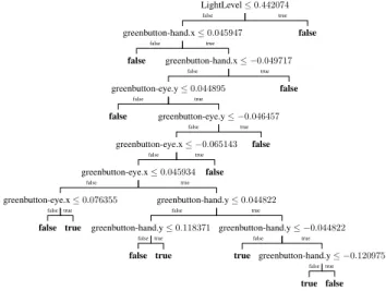
2009) C4.5 decision tree (Quinlan 1993) for symbol learn-ing. A representative learned precondition classifier for in-teracting with the green button is given in Figure 8.
A close look at the numerical values in Figure 8 suggests that, in practice, a learned set-based representation will al-ways be approximate due to sampling, even in deterministic domains with no observation noise. Thus, while our formal-ism allows an agent to learn its own symbolic representa-tion in principle, its use in practice will require a generaliza-tion of our symbol definigeneraliza-tion to probability distribugeneraliza-tions that account for the uncertainty inherent in learning. Addition-ally, it is unrealistic to hope for plans that are guaranteed to succeed—consequently future work will generalize the no-tion of feasibility to the probability of plan success.
Related Work
Several systems have learned symbolic models of the pre-conditions and effects of pre-existing controllers for later use in planning (Drescher 1991; Schmill, Oates, and Co-hen 2000; Dˇzeroski, De Raedt, and Driessens 2001; Pasula, Zettlemoyer, and Kaelbling 2007; Amir and Chang 2008; Kruger et al. 2011; Lang, Toussaint, and Kersting 2012; Mour˜ao et al. 2012). In all of these cases, the high-level
LightLevel ≤ 0.442074 false greenbutton-hand.x ≤ 0.045947 greenbutton-hand.x ≤ −0.049717 false greenbutton-eye.y ≤ 0.044895 greenbutton-eye.y ≤ −0.046457 false greenbutton-eye.x ≤ −0.065143 false greenbutton-eye.x ≤ 0.045934 greenbutton-hand.y ≤ 0.044822 greenbutton-hand.y ≤ −0.044822 greenbutton-hand.y ≤ −0.120975 false true falsetrue true false true greenbutton-hand.y ≤ 0.118371 true false falsetrue false true greenbutton-eye.x ≤ 0.076355 true false falsetrue false true false true false true false false true false true false false true false true
Figure 8: The decision tree representing the learned initia-tion set symbol for interacting with the green button. It ap-proximately expresses the set of states we might label the hand and eye are over the green button, and the light is on.
symbolic vocabulary used to learn the model were given; our work shows how to construct it.
We know of very few systems where a high-level, abstract state space is formed using low-level descriptions of actions. The most closely related work is that of Jetchev, Lang, and Toussaint (2013), which uses the same operational definition of a symbol as we do. Their method finds relational, proba-bilistic STRIPS operators by searching for symbol ground-ings that maximize a metric balancing transition predictabil-ity with model size. They are able to find small numbers of symbols in real-world data, but are hampered by the large search space. We completely avoid this search by directly deriving the necessary symbol groundings from the actions. Huber (2000) describes an approach where the state of the system is described by the (discrete) state of a set of con-trollers. For example, if a robot has three controllers, each one of which can be in one of four states (cannot run, can run, running, completed), then we can form a discrete state space made up of three attributes, each of which can take on four possible values. Hart (2009) used this formulation to learn hierarchical manipulation schemas. This approach was one of the first to construct a symbolic description us-ing motor controller properties. However, the resultus-ing sym-bolic description only fulfills our requirements when all of the low-level states in which a controller can converge are equivalent. When that is not the case—for example, when a grasp can converge in two different configurations, only one of which enables a subsequent controller to execute—it may incorrectly evaluate the feasibility of a plan.
Modayil and Kuipers (2008) show that a robot can learn to distinguish objects in its environment via unsupervised learning, and then use a learned model of the motion of the object given an action to perform high-level planning. How-ever, the learned models are still in the original state space. Later work by Mugan and Kuipers (2012) use qualitative distinctionsto discretize a continuous state space to acquire
a discrete model for planning. Discretization is based on the ability to predict the outcome of action execution.
Other approaches to MDP abstraction have focused on discretizing large continuous MDPs into abstract discrete MDPs (Munos and Moore 1999) or minimizing the size of a discrete MDP model (Dean and Givan 1997).
Discussion and Conclusions
An important implication of the ideas presented here is that actions must play a central role in determining the repre-sentational requirements of an intelligent agent: a suitable symbolic description of a domain depends on the actions available to the agent.Figure 9 shows two examples of the same robot navigating the same room but requiring different representations because it uses different navigation options.
(a) (b)
Figure 9: a) A robot navigating a room using options that move it to the centroid of each wall. Its effect sets (gray) might be described as AtLeftWall, AtRightWall, etc. b) The same robot using wall-following options. Its effect sets could be described as LowerLeftCorner, LowerRightCorner, etc.
The combination of high-level planning and low-level control—first employed in Shakey (Nilsson 1984)—is crit-ical to achieving intelligent behavior in embodied agents. However, such systems are very difficult to design because of the immense effort required to construct and interface matching high-level reasoning and low-level control compo-nents. We have established a relationship between an agent’s actions and the symbolic representation required to plan us-ing them—a relationship so close that the agent’s environ-ment and actions completely determine an appropriate sym-bolic representation, thus both removing a critical obsta-cle to designing such systems, and enabling agents to au-tonomously construct their own symbolic representations.
Acknowledgements
We thank Greg Lewis, Siddharth Srivastava, and LIS for in-sightful conversations. GDK was supported in part by an MIT Intelligence Initiative Fellowship. This work was sup-ported in part by the NSF under Grant No. 1117325. Any opinions, findings, and conclusions or recommendations ex-pressed in this material are those of the author(s) and do not necessarily reflect the views of the National Science Foundation. We also gratefully acknowledge support from ONR MURI grant N00014-09-1-1051, from AFOSR grant FA2386-10-1-4135 and from the Singapore Ministry of Edu-cation under a grant to the Singapore-MIT International De-sign Center.
References
Amir, E., and Chang, A. 2008. Learning partially observable deter-ministic action models. Journal of Artificial Intelligence Research 33:349–402.
Barto, A., and Mahadevan, S. 2003. Recent advances in hierar-chical reinforcement learning. Discrete Event Dynamic Systems 13:41–77.
Burridge, R.; Rizzi, A.; and Koditschek, D. 1999. Sequential com-position of dynamically dextrous robot behaviors. International
Journal of Robotics Research18(6):534–555.
Cambon, S.; Alami, R.; and Gravot, F. 2009. A hybrid approach to intricate motion, manipulation and task planning. International
Journal of Robotics Research28(1):104–126.
Choi, J., and Amir, E. 2009. Combining planning and motion planning. In Proceedings of the IEEE International Conference on Robotics and Automation, 4374–4380.
Dean, T., and Givan, R. 1997. Model minimization in Markov decision processes. In In Proceedings of the Fourteenth National Conference on Artificial Intelligence, 106–111.
Dornhege, C.; Gissler, M.; Teschner, M.; and Nebel, B. 2009. Inte-grating symbolic and geometric planning for mobile manipulation. In IEEE International Workshop on Safety, Security and Rescue Robotics.
Drescher, G. 1991. Made-Up Minds: A Constructivist Approach to Artificial Intelligence. MIT Press.
Dˇzeroski, S.; De Raedt, L.; and Driessens, K. 2001. Relational reinforcement learning. Machine learning 43(1):7–52.
Ghallab, M.; Nau, D.; and Traverso, P. 2004. Automated planning: theory and practice. Morgan Kaufmann.
Hall, M.; Frank, E.; Holmes, G.; Pfahringer, B.; Reutemann, P.; and Witten, I. 2009. The WEKA data mining software: An update.
SIGKDD Explorations11(1):10–18.
Hart, S. 2009. The Development of Hierarchical Knowledge in Robot Systems. Ph.D. Dissertation, University of Massachusetts Amherst.
Hoffmann, J., and Nebel, B. 2001. The FF planning system: Fast plan generation through heuristic search. Journal of Artificial
In-telligence Research14:253–302.
Huber, M. 2000. A hybrid architecture for hierarchical reinforce-ment learning. In Proceedings of the 2000 IEEE International Con-ference on Robotics and Automation, 3290–3295.
Jetchev, N.; Lang, T.; and Toussaint, M. 2013. Learning grounded relational symbols from continuous data for abstract reasoning. In Proceedings of the 2013 ICRA Workshop on Autonomous Learning. Kaelbling, L., and Lozano-P´erez, T. 2011. Hierarchical planning in the Now. In Proceedings of the IEEE Conference on Robotics and Automation.
Kocsis, L., and Szepesv´ari, C. 2006. Bandit based Monte-Carlo planning. In Proceedings of the 17th European Conference on Ma-chine Learning, 282–293.
Konidaris, G., and Barto, A. 2009a. Efficient skill learning using abstraction selection. In Proceedings of the Twenty First Interna-tional Joint Conference on Artificial Intelligence.
Konidaris, G., and Barto, A. 2009b. Skill discovery in continuous reinforcement learning domains using skill chaining. In Advances in Neural Information Processing Systems 22, 1015–1023. Kruger, N.; Geib, C.; Piater, J.; Petrick, R.; Steedman, M.; W¨org¨otter, F.; Ude, A.; Asfour, T.; Kraft, D.; Omrˇcen, D.;
Agos-tini, A.; and Dillmann, R. 2011. Object-action complexes:
Grounded abstractions of sensory-motor processes. Robotics and
Autonomous Systems59:740–757.
Lang, T.; Toussaint, M.; and Kersting, K. 2012. Exploration in re-lational domains for model-based reinforcement learning. Journal
of Machine Learning Research13:3691–3734.
Lozano-Perez, T.; Mason, M.; and Taylor, R. 1984. Automatic synthesis of fine-motion strategies for robots. International Journal
of Robotics Research3(1):3–24.
Malcolm, C., and Smithers, T. 1990. Symbol grounding via a hybrid architecture in an autonomous assembly system. Robotics
and Autonomous Systems6(1-2):123–144.
McDermott, D.; Ghallab, M.; Howe, A.; Knoblock, C.; Ram, A.; Veloso, M.; Weld, D.; and Wilkins, D. 1998. PDDL—the planning domain definition language. Technical Report CVC TR98003/DCS TR1165, Yale Center for Computational Vision and Control. Modayil, J., and Kuipers, B. 2008. The initial development of object knowledge by a learning robot. Robotics and Autonomous
Systems56(11):879–890.
Mour˜ao, K.; Zettlemoyer, L.; Patrick, R.; and Steedman, M. 2012. Learning STRIPS operators from noisy and incomplete observa-tions. In Proceedings of Conference on Uncertainty in Articial In-telligence.
Mugan, J., and Kuipers, B. 2012. Autonomous learning of high-level states and actions in continuous environments. IEEE
Trans-actions on Autonomous Mental Development4(1):70–86.
Munos, R., and Moore, A. 1999. Variable resolution discretiza-tion for high-accuracy soludiscretiza-tions of optimal control problems. In Proceedings of the Sixteenth International Joint Conference on Ar-tificial Intelligence, 1348–1355.
Nilsson, N. 1984. Shakey the robot. Technical report, SRI Interna-tional.
Pasula, H.; Zettlemoyer, L.; and Kaelbling, L. 2007. Learning symbolic models of stochastic domains. Journal of Artificial
Intel-ligence Research29:309–352.
Precup, D. 2000. Temporal Abstraction in Reinforcement Learning. Ph.D. Dissertation, Department of Computer Science, University of Massachusetts Amherst.
Quinlan, J. 1993. C4.5: programs for machine learning, volume 1. Morgan Kaufmann.
Schmill, M.; Oates, T.; and Cohen, P. 2000. Learning planning operators in real-world, partially observable environments. In Pro-ceedings of the Fifth International Conference on Artificial Intelli-gence Planning and Scheduling, 245–253.
Sutton, R.; Precup, D.; and Singh, S. 1999. Between MDPs and semi-MDPs: A framework for temporal abstraction in reinforce-ment learning. Artificial Intelligence 112(1-2):181–211.
Tedrake, R. 2009. LQR-Trees: Feedback motion planning on
sparse randomized trees. In Proceedings of Robotics: Science and Systems, 18–24.
Wolfe, J.; Marthi, B.; and Russell, S. J. 2010. Combined Task and Motion Planning for Mobile Manipulation. In International Conference on Automated Planning and Scheduling.