Practical design rules for single-channel ultra high-speed dense dispersion management telecommunication systems

HAL Id: hal-00474467

https://hal.archives-ouvertes.fr/hal-00474467

Submitted on 20 Apr 2010

HAL is a multi-disciplinary open access

archive for the deposit and dissemination of sci-entific research documents, whether they are pub-lished or not. The documents may come from

L’archive ouverte pluridisciplinaire HAL, est destinée au dépôt et à la diffusion de documents scientifiques de niveau recherche, publiés ou non, émanant des établissements d’enseignement et de

Practical design rules for single-channel ultra high-speed

dense dispersion management telecommunication

systems

Julien Fatome, Coraline Fortier, Stéphane Pitois

To cite this version:

Julien Fatome, Coraline Fortier, Stéphane Pitois. Practical design rules for single-channel ultra high-speed dense dispersion management telecommunication systems. Optics Communications, Elsevier, 2009, 282 (7), pp.1427-1434. �hal-00474467�

Practical design rules for single-channel ultra

high-speed Dense Dispersion Management

Telecommunication systems

J. Fatome, C. Fortier and S. Pitois

Institut Carnot de Bourgogne, UMR 5209 CNRS-Université de Bourgogne, 9 av. Alain Savary, BP 47870, 21078 Dijon, France

Author e-mail address: Julien.Fatome@u-bourgogne.fr

Abstract: In this work, we establish some efficient and practical design rules for the

implementation of single-channel ultra-high speed (>160-Gbit/s) telecommunication systems based on dense dispersion management. Moreover, we analyze some of actual implementation issues such as slope compensation scenario, junction losses, polarization mode dispersion and chromatic dispersion fluctuations.

I. INTRODUCTION

For more than ten years, transmission of information in optical fiber systems at bit rates per channel higher than 160 Gbit/s has been subject to a large number of numerical and experimental investigations [1]-[2]. At such bit rates, fiber dispersion becomes one of the dominant limiting effects and the implementation of a dispersion compensation scenario is usually necessary to ensure that each pulse remains trapped in its bit slot when the optical signals reach the receiver. Basically, two dispersion management techniques have been reported in the literature. The first one, referred as “conventional dispersion management”, consists of compensating for the dispersion of the transmission fiber (typically single mode fiber SMF) at the end of each amplification span. In such pseudo-linear systems, input pulses broaden rapidly and spread over a large number of neighboring bits. The propagation distance is therefore mainly limited by

intrachannel nonlinear effects such as intrachannel four wave mixing (IFWM) or intrachannel cross-phase modulation (IXPM) [3]-[5]. The second technique, known as “dense dispersion management” (DDM), consists of alternating the fiber dispersion over distances much shorter than the amplification span (typically every kilometer) [6]-[7]. In such systems, pulses propagate with a strongly reduced breathing, leading to a significant reduction of the intrachannel interactions [6]. This DDM technique was then considered in several numerical and experimental investigations [6]-[22]. In particular Maruta et al. were first to experimentally demonstrate the capacity of this kind of transmission regime through the propagation of a 87-GHz pulse train [12]. In 2003, Fatome et al. have also demonstrated the potential of the DDM technique for 160-Gbit/s applications through the propagation of a 160-GHz pulse train on 900 km in a commercially available NZ-DSF fiber based dispersion map [13]. In parallel, dense dispersion fibers called “perfect cables” because of their spliceless feature were also developed to overcome the practical implementation issue provided by the concatenation of a large number of fiber sections and in particular the resulting splicing losses [14], [17]-[18]. The drawing process of this kind of DDM fibers was demonstrated in refs. [14], [17]-[18] and lead to the first and only experimental system result of a 100-Gbit/s transmission on 1000 km [14]. More recently, a comparison between the DDM and quasi-linear regimes at 160 Gbit/s has been also reported in ref. [19], showing that DDM transmission lines, which allow much longer propagation distance in a single-channel configuration than pseudo-linear systems, could suffer from strong interchannel nonlinear interactions in the wavelength division multiplexed (WDM) configuration. However, in ref. [20], Shtaif has shown that these interchannel penalties could be removed by using a two-fold periodicity but in the cost of the DDM map simplicity. Nevertheless, another practical advantage of DDM system is that the information is available at each dispersion managed cell (typically every kilometer) whereas in pseudo-linear systems, pulses are recovered only at the end of the amplification span (typically 100 km). This property could find significant interest in some specific systems, for example in a network configuration where the signal could be plugged in or picked up at almost any point of the line. Therefore, we believe that some efforts remain to be done in order to better understand the basic properties of DDM systems. Indeed, although many analytical and numerical studies have been published on the DDM technique, the design rules remain generally either complicated, large numerical time consuming, sometimes simply inaccurate and most often far from the real implementation issues. Consequently, it is

worth noting that very few experimental results follow from these studies. In this context, we propose to establish and demonstrate in this work some analytical and practical simple rules for the design of single-channel DDM fiber systems and to numerically study some of actual implementation issues such as slope compensation scenario, polarization mode dispersion, junction losses and chromatic dispersion fluctuations.

II. ANALYTICAL DESIGN RULES

2.1 Optimum number of fiber sections

The DDM system studied in this work is schematically described in Fig. 1. It consists of an amplification span of Za=50 km made of a concatenation of N fiber sections (L1≈L2) with

opposite dispersions of +/-D and an average dispersion dm. The third order dispersion is taken into account and slopes could have the same or opposite signs depending on the study. The fiber has an effective area of 55 µm2 and typical high losses of α = 0.3 dB/km due to the prototype nature of this kind of fiber. The amplification stage is ensured by an Erbium doped fiber amplifier (noise figure of 4.5 dB) followed by a 1-THz flat-top optical filter to avoid the accumulation of spontaneous noise emission during the propagation. The transmitted signal consists of a return-to-zero (RZ) 160-Gbit/s pseudo-random bit-sequence (prbs) of 2048 bits with Gaussian pulses having a full width at half maximum of FWHM0=1.5ps. Polarization mode dispersion (PMD) is

taken into account thereafter.

The design rules of the system are based on an original idea developed by Mamyshev in ref. [23] and extended here to the DDM implementation. Basically, as illustrated in Fig.1b, in a densely dispersion managed system, the map length being much shorter than the amplifier span, pulses propagate with a strongly reduced breathing compared with the case of a conventional dispersion management system [6]-[11]. Following the observation that the pulse breathing is limited to the first neighboring bit-slots, and in order to determine the optimum number of fiber sections contained in our system N=Nopt, we have to found a criterion which minimizes only the

nonlinear interactions between first adjacent pulses. To this aim, as proposed by Mamyshev in ref. [23] for classical dispersion management systems, we shall consider the nonlinear phase of a pulse P1(t) overlapped during its propagation by a neighboring pulse P2(t). In order to apply and

extend the Mamyshev method to the case of DDM system, we will consider not only the cross phase modulation effect (XPM) but also the self phase modulation (SPM) undergone by pulses

during their propagation and minimize the total shift of the instantaneous frequency occurring during the whole DDM amplifier span propagation.

z_a +D, L₁ D (ps/km.nm) -D , L₂ 0 A ≈ dm Filter z_a z_a +D, L₁ D (ps/km.nm) -D , L₂ 0 A ≈ dm Filter P z t P z t

Fig. 1. (a) Dense Dispersion Management system set-up (b) Illustration of pulse breathing occurring during the propagation of pulses in a DDM system.

We consider two neighboring Gaussian pulses P1_0(t) and P2_0(t) with electric field A1_0(t) and

A2_0(t) separated by T=6.25 ps corresponding to a bit rate of 160-Gbit/s and defined as:

( )

( )

(

)

( )

( )

(

(

)

)

with t0=FWHM0/2ln(2)1/2, FWHM0 being the full width at half-maximum at z=0.

During its propagation on dz in the DDM system, the cumulated nonlinear phase of P1(t) is given

by:

( )

(

( )

( )

)

(

( )

( )

)

( )

(

( )

)

( )

(

( )

)

where β2 is the chromatic dispersion of the first fiber segment and ω the angular pulsation. The

instantaneous frequency shift dΔf integrated on P1(t) propagating on dz is then given by:

dz dt P dt P dt dP dt dP f d

∫

∫

where we have multiplied the top term by P1 so as to balance the nonlinear effects by the number

of photons of P1(t) concerned by the overlapping interaction.

If we now calculate the total instantaneous frequency shift Δf undergone by P1(t) along the

amplification span we obtain the following relation:

dz dt P dt P dt dP dt dP N f L

∫

∫

_∫

Figure 2 represents Δf integrated over the whole amplification span as a function of the maximum pulse broadening ε=FWHM/FWHM0 occurring in the line at ~L1/2=Za/2N and normalized by the

bit slot T.

Fig. 2. Instantaneous frequency shift as a function of maximum pulse broadening occurring in the line.

We can see in Fig. 2 that the evolution of Δf is dramatically different that the results obtained in ref. [23] by Mamyshev. For very weak pulse broadening, pulses propagate in a quasi soliton regime and consequently the SPM effect dominates. Then, when the maximum of pulse broadening increases and pulses begin to overlap, we can see that the total instantaneous frequency shift decreases until a minimum obtained for ε=0.55. This phenomenon can be explained by the decrease of the average peak power due to pulse broadening and thus the decrease of SPM, but also by the fact that SPM and XPM have an opposite sign when pulses began to overlap. For pulse broadening larger than ε=0.55, the XPM effect begin to dominate and reach a maximum for ε=1.5 where maximum of nonlinear interactions occur. Note that for broadening larger than 3, the model is not still valid because pulses begin to overlap on several

neighboring pulses and thus, we fall in a classical dispersion managed system mainly rules by IFWM [3]-[4].

The maximum pulse width (FWHM) achieved by a Gaussian pulse having an initial pulse width FWHM0 and propagating in our DDM line is obtained at ~L1/2 and is given by [24]:

2 0 2 1 0 1 ₂ 1 ₂ ⎟⎟ ⎠ ⎞ ⎜⎜ ⎝ ⎛ + = ⎟⎟ ⎠ ⎞ ⎜⎜ ⎝ ⎛ + = d a d NL z FWHM L L FWHM FWHM , (6)

where Ld is the dispersion length given by [24]:

2 2 2 0 665 . 1 β FWHM Ld = . (7)

By introducing the condition on ε in equation 6, we can now calculate the optimum and worst number of fiber sections N as a function of fiber dispersion of the line and initial pulse width thanks to the following relation:

1 2 2 0 − ⎟⎟ ⎠ ⎞ ⎜⎜ ⎝ ⎛ = FWHM T L z N d a ε , (8)

where ε = 0.55 for the optimum fiber line Nopt and ε = 1.5 for the line to avoid Navoid. Note that

linear and local losses could be taken into account in relation (5) but would not change the optimum line.

In order to valid our approach, we have simulated the DDM system illustrated in Fig. 1a so as to find the optimum and worst number of fiber sections for different couple of fiber dispersions +/- D. Numerical simulations have been performed by means of the VPI transmission maker software using a classical split step Fourier algorithm. The third-order dispersion is in-line managed by means of fiber sections with opposite slope S = +/- 0.07 ps/km.nm2. Polarization mode dispersion is still neglected. Fig. 3a shows a typical performance-map obtained for D = +/-3 ps/km.nm. This map represents the maximum transmission distance defined as the maximal propagation distance where the usual Q-factor still remains larger than 6 as a function of the number of sections N contained in the DDM amplifier span as well as average power. The average chromatic dispersion of the line was derived for each simulation by means of the method described bellow in section 1.2. For a number of fiber sections below N < 40, we can see a white

area where the transmission distance remains under 1000 km with a minimum of performances obtained for Navoid = 20. At the opposite, when N > 50, the transmission distance remains larger

than 2000 km with an optimum (2700 km) number of fiber sections equal to Nopt = 60 (L1 ≈ L2 ≈

830 m) for an average power of Popt = 5.5 dBm. Note that the number of fiber sections is not a

critical parameter and presents a large tolerance around Nopt where performances remain larger

than 2500 km, which is a great advantage for practical implementation.

Fig. 3. (a) Performance-map for the D = +/- 3 ps/km.nm, S = +/- 0.07 ps/km.nm2 DDM line as a function of number of fiber sections and average power (b) Q-factor as a function of distance for the optimum (N=60) and to avoid (N=20) D = +/-3 ps/km.nm, S = +/-0.07 ps/km.nm2 DDM line as well as for a classical SMF/DCF line

For illustration, we have plotted in Fig. 3b the usual Q-factor as a function of distance for the optimum 60- and to avoid 20-fiber-sections D = +/- 3 ps/km.nm, S = +/- 0.07 ps/km.nm2 DDM line found in Fig. 3a as well as for a typical example of dispersion managed fiber line made of 100 km of single mode fiber (SMF, D = 17 ps/km.nm, S = 0.07 ps/km.nm, Aeff = 80 µm² and α = 0.2 dB/km) followed by 17 km of dispersion compensating fiber (DCF, D = -100 ps/km.nm, S = -0.41 ps/km.nm, Aeff = 30 µm² and α = 0.6 dB/km) [25]. The amplification stages are ensured by two EDFA and two 1-THz flat-top filters while the optimum average power was found to be P = 5.9 dBm [25]. As we can see, a large improvement is reached for the optimum Nopt = 60 DDM

line while the Navoid = 20 DDM and classical SMF/DCF-lines merely provide identical

performances. This last result underlines the fact that the number of fiber sections and thus the design of the line must be carefully chosen in the sense that increasing the number of fiber segments is not sufficient to improve the performances of the system and can even be worst than a classical SMF/DCF transmission line as shown in Fig. 3b.

(a)

In order to valid the relation (8), we have completed the same performance-map as shown in Fig. 3a for several values of fiber dispersion in the range of 0-5 ps/km.nm and reported in Fig. 4a the optimum (circles) and to avoid (stars) number of fiber sections N as well as our theoretical predictions provided by equation (8), (dashed-line). As can be seen, a great agreement between theoretical and numerical results is achieved proving the validity of our calculations. Moreover, to illustrate the tolerance in terms of optimum fiber sections, we have also plotted tolerance bars showing the number of fiber sections that allow at least 90% of the maximum transmission distance. As can be seen, a comfortable tolerance around Nopt is obtained, which is compatible

with fiber manufacturing processes. Finally, in order to give an overview of the fiber to be drawn, we have also plotted in Fig. 4b the fiber length section corresponding to the results of Fig. 4a. The numerical and theoretical results are simply obtained by the relation (L1≈L2≈Za/N).

Fig. 4. (a) Numerical results: Optimum (circles) and to avoid (stars) number of fiber sections as a function of fiber dispersion. Dashed-lines: theoretical predictions given by relation (8). Tolerance bars: number of fiber sections allowing at least 90% of the maximum transmission distance (b) Length of fiber sections corresponding to the results of Fig. 4a.

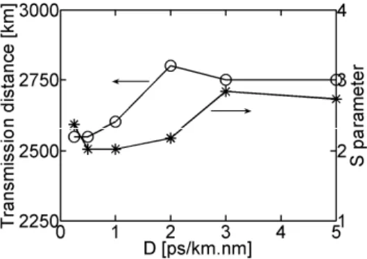
Figure 5 complete the numerical results obtained in Fig. 4a for the optimum number of fiber sections. We can see that the maximum transmission distance (circles) is merely constant as a function of dispersion but it would be suitable to choose a dispersion value above 2 ps/km.nm in order to be less sensitive to the third order chromatic dispersion and dispersion fluctuations. We have also indicated in Fig. 5 the corresponding optimum S parameter (stars) often used in the literature and given by:

2 0 2 _ 2 2 1 _ 2 1 ) ( FWHM L L S= β − β . (9)

We can see that the usual S parameter is merely found around 2.5 and not equal to 1.65 as often mentioned in the literature [26]. We attribute this observation to the fact that the S = 1.65 rule was obtained by means of the collision distance calculation between two neighboring pulses which we believe is no suitable to optimize a DDM system.

Fig. 5. Numerical results: Maximum transmission distance (circles) and S parameter (stars) as a function of fiber dispersion for the optimum number of fiber section Nopt found in Fig. 4a.

2.2 Optimum average dispersion

It has been shown in previous works that a slight positive average dispersion can substantially improve the performance of the dispersion-managed transmission line [7]. This property is illustrated in Fig. 6a where we have plotted the evolution of the maximum transmission distance of the D = +/- 3 ps/km.nm 60-sections DDM fiber as a function of the average dispersion of the line for an average power of Popt = 5.5 dBm (stars). As can be seen, the maximum transmission

distance is increased by nearly a factor two simply by optimizing the amount of residual dispersion.

Fig. 6. (a) Maximum transmission distance (Q>6) as a function of the average dispersion for the D = +/- 3 ps/km.nm, S = +/- 0.07ps/km.nm2, DDM line and Popt =

5.5 dBm. The circle is the optimum average dispersion obtained from the collective variables technique whereas the square is obtained from the numerical method of Fig. 6b. (b) Evolution of the normalized Δ parameter as a function of the average dispersion of the D = +/- 3 ps/km.nm, S = +/- 0.07ps/km.nm2, DDM line and Popt =

5.5 dBm.

Therefore, in this section, we will focus our attention on indicating a way so as to simply and rapidly determine the optimum average dispersion of the DDM line. To this aim, we will compare our method to two other techniques to estimate this optimal value. The first one consists of simulating the signal propagation as in Fig. 6a (stars) and calculating the Q-factor for each value of the average dispersion [7]. Since it models the system as accurately as possible, this method is the most reliable but is in general large numerical time consuming. To overcome this drawback, some analytical methods have been developed, mainly based on variational techniques. For example, in a recent paper, Nakkeeran et al. have derived an analytical method based on collective variables to obtain an estimation of the optimum average dispersion [20]-[22]. By applying this method to our system, we have instantaneously obtained the value indicated by a circle in Fig. 6a. A good agreement with numerical simulations is obtained, illustrating the efficiency of this analytical approach. But, because such an analytical technique can be difficult to implement in practice, we have finally considered a simple numerical method based on the propagation of a single optical pulse. More precisely, we will consider an isolated optical pulse of our signal propagating in a single amplification span and will maximize the correlation between the input and output pulses as a function of the average dispersion. At the end of the span, we estimate the transmission quality by using the following correlation parameter:

∫

φ

α

where α is the linear fiber losses, u(t) the electric field and φa is a phase offset chosen so that the two complex fields have the same phase at the center of the bit slot. Figure 6b shows the evolution of Δ (in normalized units) as a function of the average dispersion of the D = +/-3-ps/km.nm, 60-sections, Popt = 5.5 dBm DDM line. The minimum Δ value (square in Fig. 6a),

agreement with the values obtained from the previous methods and thus provides a good estimation of the optimum average group-velocity dispersion. Note that this simple technique, as well as the collective variables approach, is efficient as long as the interaction between neighboring adjacent pulses can be neglected.

III. INFLUENCE OF DISPERSION FLUCTUATIONS

As pointed out in refs. [17], [27]-[28], dispersion of fiber sections can fluctuate along the line due to the extreme sensitivity of the DDM fiber drawing process or simply because of the influence of surroundings [27]-[28] and thus could lead to pulse broadening and signal degradations [29]-[30]. In this section, we analyze the influence of this phenomenon on the performance of the optimum D = +/-3 ps/km.nm, 60-sections DDM line. Note that third-order chromatic dispersion is in-line managed by means of fiber sections with opposite slope S = +/- 0.07 ps/km.nm2. The dispersion fluctuations are modeled at any point of the amplification span by adding a random amount of chromatic dispersion ΔD(z) to the local dispersion Dth = +/-D. ΔD(z) has a 0-mean

value and is modeled by a sum of 10 sinusoidal functions which period and phase are randomly chosen. At any point of the line, the chromatic dispersion is given by D

( )

( )

( )

_∑

where K_n∈

[

]

[

]

Kn is randomly drawn in the interval [50 :1000] so as to take into account both rapid and slow

fluctuations of chromatic dispersion, thus, the 10 sinusoidal functions have spatial periods comprised between 50 m (Kn = 1000) and 1 km (Kn = 50). The random phase φn allows us to

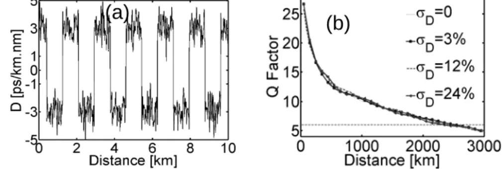
decorrelate the 10 functions and thus to avoid any cumulative effect. U is kept constant for the 10 sinusoidal functions so as to not emphasize any regime of fluctuations. Figure 7a shows an example of the D = +/- 3 ps/km.nm 60-sections DDM line degraded by a σD = 24% dispersion

variation. Then, we have simulated the propagation of the 160-Gbit/s signal in the degraded line as a function of the dispersion fluctuation amplitude for Popt = 5.5 dBm. The results are averaged

on 10 runs of degraded line so as to avoid any dramatic event. The performances of the system as a function of σD are presented in Fig. 7b. We can observe that the random fluctuations of

chromatic dispersion do not affect the quality of the transmission, even for fluctuations as large as 24% providing that the average value of chromatic dispersion is kept to its initial value and that the fluctuation period is much smaller than the nonlinear length so as to not perturb the DDM soliton.

Fig. 7. (a) Typical segment of the +/- 3 ps/km.nm 60-sections DDM line

degraded by a 24% random variation of the dispersion (b) Q-factor as a function of distance for different dispersion variation amplitudes and for an average power of 5.5 dBm.

IV. INFLUENCE OF SLOPE COMPENSATION SCENARIO

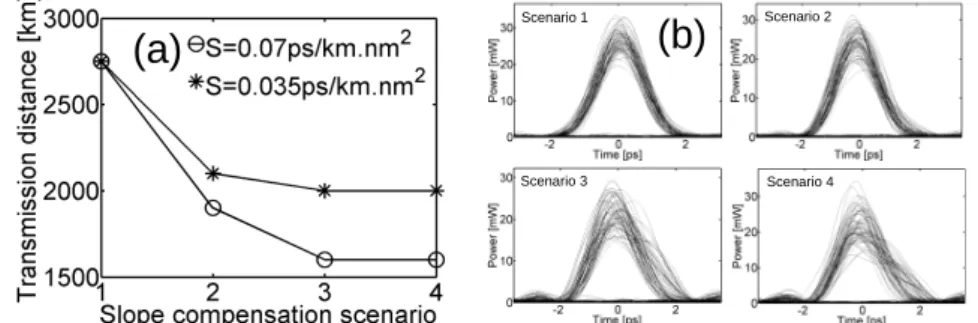
Although it was demonstrated in ref. [14], it seems technically difficult during the drawing process to achieve a slope management by means of opposite slope fiber sections. Consequently, manufacturers would often prefer to minimize a fixed value of the line dispersion slope [17]-[18]. It’s the reason why, we have considered in this section several scenarios of slope compensation by means of additional lumped negative-slope modules [13], [31]. Figure 8a shows the maximum transmission distance (Q>6) of the optimum D = +/- 3-ps/km.nm, 60-sections, Popt = 5.5-dBm, S

= 0.07-ps/km.nm2 and S = 0.035-ps/km.nm2 DDM system for an in-line slope management with fiber sections of opposite slope (scenario 1), for an end-line compensation by means of a module localized at the amplification site which compensates for the total third-order chromatic dispersion (TOD) (scenario 4), for the same module localized in the middle of the line (scenario 3) and for two modules which compensates for half of the third-order dispersion localized at 1/3 and 2/3 of the line (scenario 2). For these simulations, the module has been supposed to be lossless. We can see in Fig. 8a that the transmission distance is largely reduced without an in-line slope compensation (1600 km for scenario 4 vs 2700 km) even with a weak slope value of S = 0.035 ps/km.nm2. As shown in Fig. 8b, which illustrates the eye-diagrams of the 160-Gbit/s signal after 1000 km of propagation for the 4 different scenarios, this behavior is largely due to

(a)

severe asymmetric distortions undergone by pulses during the propagation and that, even for a linear perfect slope compensation. This phenomenon was already observed in ref. [31] and could be explained by the fact that pulses propagate on numbers of TOD length Ld3 [24]:

3 3 3 0 3 665 . 1 β FWHM L_d = . (12)

Typically, pulses propagate on more than 8 Ld3 with a 0.07-ps/km.nm2 dispersion slope in a

50-km span and thus undergone large asymmetries which increase nonlinear interactions between neighboring pulses. These asymmetries modify the pulse spectrum through self-phase modulation and tend to increase the dispersion slope effect compare to a linear propagation regime which consequently, changing the amount of TOD to be compensated. These observations underline the practical issue of slope compensation in presence of nonlinear effects.

Scenario 1 Scenario 3 Scenario 2 Scenario 4 Scenario 1 Scenario 3 Scenario 2 Scenario 4

Fig. 8. (a) Maximum transmission distance for the D = +/-3 ps/km.nm, 60-sections, 5.5-dBm DDM line for the 4 different slope compensation scenarios (b) Eye-diagrams of the 160-Gbit/s signal after 1000 km of propagation for the 4 different slope compensation scenarios and for an average power of 5.5 dBm.

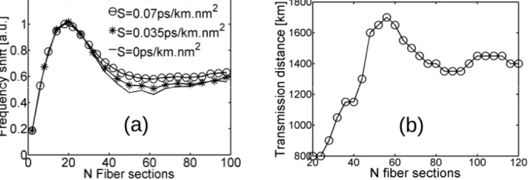
Meanwhile, despite the increase of nonlinear interactions between adjacent pulses due to pulse asymmetry, we have found by including the third order dispersion in relations (3) and by integrating the instantaneous frequency shift dΔf on the whole span of amplification Za that

scenario slope compensation does not affect the choice of the optimum fiber line. In order to clarify this point, we have plotted in Fig. 9a the total instantaneous frequency shift as a function of the number of fiber sections contained in the D = +/-3 ps/km.nm fiber line for an end-line slope compensation scenario. We can see that for S = 0.035 or 0.07 ps/km.nm2_{, the optimum}

number of fiber sections Nopt is still around 60 as found in Fig. 4a for an in-line slope

compensation. We have then verified this theoretical prediction by numerical simulations. Figure

(b)

(a)

9b shows the maximum transmission distance (Q>6) as a function of the number of fiber sections for the D = +/- 3 ps/km.nm, S = 0.07 ps/km.nm2 fiber line with an end-line slope compensation (scenario 4) and for an input average power of 5.5 dBm. These numerical results are in agreement with theoretical predictions of Fig. 9a. Even if the maximum transmission distance is dramatically reduced compare to in-line slope compensation (1600-vs-2700 km), the maximum transmission distance is still obtained for 60 segments of fiber. This point is interesting for the fiber designer who is free to take into account the third order chromatic dispersion for the design of the line and keep a degree of freedom for the choice of the slope compensation scenario.

Fig. 9. (a) Instantaneous frequency shift as a function of the number of fiber sections in the D = +/- 3 ps/km.nm line for a end-line slope compensation configuration (b) Maximum transmission distance as a function of the number of fiber sections in the D = +/- 3 ps/km.nm, S = 0.07ps/km.nm2 DDM line for a end-line slope compensation configuration and for an average power of 5.5 dBm.

V. INFLUENCE OF OPTICAL LOSSES

As mention in ref. [17], manufacturing a dense dispersion cable by means of an outer diameter variation of the drawing fiber or thanks to an assembly of preform canes, could lead to additional losses at section junctions. In another hand, since it seems complicated to draw a DDM fiber including both second- and third-order dispersion compensation, one could prefer designing a DDM line simply by splicing a couple of fibers with suitable and well-known parameters [12]-[13]. In both cases, it is then interesting to study the influence of junction losses on the optimum dispersion map. Even if we can add the local losses of the system in the model described in section 1, it seems difficult to compare the different dispersion maps as a function of the number of fiber sections because the optimum average power will increase with the total losses of the system. In this context and in order to give an overview of the different parameters influencing

(b)

(a)

the system performances, we have first completed a performance map of the D = +/- 3 ps/km.nm, S = +/- 0.07 ps/km.nm2 fiber line where we have included a 0.1-dB loss at each fiber junction. Results are plotted in Fig. 10a and show that, compared to Fig. 3a (without junction loss), the area in which the performances of the system are maximized is largely reduced and slightly shifted towards the lower number of fiber sections. The maximum transmission distance is reduced to 1600 km (vs 2700 km in the lossless junction case) and was still obtained as in Fig. 3a for Nopt = 60 (L1 ≈ L2 ≈ 830 m) and for an average power of 9 dBm, meaning that the junction

losses are not critical for the design of the line and thus could be neglected during the conception process. Then, in order to take into account the increase of average power in our model, we have realized a linear fit of the optimum average power as a function of the number of fiber sections contained in the line. The resulting fit is plotted on Fig. 10a in dashed-line. We have included in equation (5) the junction losses and corresponding optimum average power and integrating the instantaneous frequency shift dΔf on the whole span of amplification Za. Results are illustrated in

Fig. 10b. The shape of the curve is quite different than in Figs. 2 and 9a and can be explained by the exponential increase of the peak power as a function of the number of fiber sections due to the host of fiber section losses. However, if we exclude the first part of the curve where IFWM, which is not taking into account, is the nonlinear limiting effect, we can observe that the minimum of interaction is obtained around 50 fiber sections in agreement with the numerical results of Fig. 10a and not so far from the lossless junction case described in Figs. 2 and 9a.

Fig. 10. (a) Performance-map of the D = +/- 3 ps/km.nm, S = +/- 0.07 ps/km.nm2 _{DDM line including 0.1 dB losses at fiber junctions as a}

function of number of fiber sections and average power; the dashed-line corresponds to a linear fit of the optimum average power (b) Instantaneous frequency shift as a function of the number of fiber sections in the D = +/-3 ps/km.nm, S = +/-0.07 ps/km.nm2 DDM line including 0.1 dB losses at fiber junctions and for an average power given by the linear fit of Fig. 10a.

(a)

VI. INFLUENCE OF POLARIZATION MODE DISPERSION

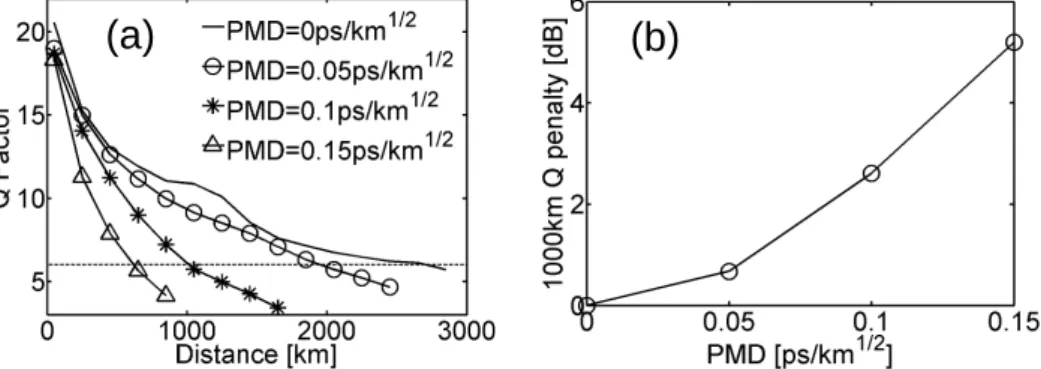
In this last section, we have focused our attention on the influence of the polarization-mode-dispersion (PMD) on the DDM system performances. It is now well known that at bit rates higher than 40 Gbit/s, PMD emerges as a key limitation in already installed optical fiber transmission systems [32] due to large pulse distortion and broadening [33]-[34] and thus should be one of the key parameter for future generation of fibers. In this context, we have studied the influence of the amount of PMD on the performances of the optimum D = +/- 3 ps/km.nm, S = +/- 0.07 ps/km.nm2_{, 60-sections, 5.5-dBm DDM line. In our simulations, PMD was modeled using the}

standard coarse-step method based on the numerical integration of two coupled nonlinear Schrödinger equations in randomly varying birefringent short fiber sections [33]-[34]. Note that in order to take into account for the stochastic feature of the PMD effect, each point was obtained by averaging the Q-factor over 100 realizations.

Figure 11a shows the evolution of the Q-factor as a function of propagation distance for several values of the line PMD. Dramatically, we found that the transmission distance, compare to the 0-PMD line, is divided by more than 2 and 3 for reasonable prototype fiber values of 0.1 ps/km1/2 and 0.15 ps/km1/2. Indeed, the Q-factor penalty, represented in Fig. 11b, reaches almost 3 and 6 dB after only 1000 km of propagation. We can conclude that the PMD of the DDM fiber has to be less than 0.05 ps/km1/2 _{to prevent any dramatic degradation or has to be compensated to}

keep its benefits compared to a classical SMF/DCF map.

Fig. 11. (a) Q-factor as a function of distance for different PMD values of the D = +/- 3 ps/km.nm, S = +/- 0.07 ps/km.nm2, 5.5-dBm, 60-sections DDM line (b) Corresponding Q-penalty after 1000km of propagation as a function of PMD.

(b)

(a)

VII. CONCLUSION

In this work, we have established and demonstrated some analytical and practical simple rules for the design of single-channel ultra-high speed (>160-Gbit/s) telecommunication systems based on special dense dispersion management drawn fiber. We have also numerically studied some of practical implementation issues such as the slope compensation scenario, the influence of dispersion fluctuations along the line, the junction losses and polarization mode dispersion. We have found that the slope compensation scenario and junction losses could be neglected for the design of the line, that moderate random chromatic dispersion fluctuations do not provide any signal degradation and that polarization mode dispersion will be a key parameter during the drawing process. Finally, following our rules, the ideal 160-Gbit/s DDM line would have a number of fiber sections which chromatic dispersion provides a maximum pulse broadening of 0.55 times the bit-slot, a third order dispersion compensation with fiber section of opposite slope is recommended and the PMD must be kept below 0.05 ps/km1/2 to allow transmission distances larger than 2000 km.

VIII. ACKNOWLEDGMENT

We would like to acknowledge financial support of the Agence Nationale de la Recherche (FUTUR project).

IX. REFERENCE

[1] M. Nakazawa, H. Kubota, K. Suzuki, E. Yamada, and A. Sahara, "Ultrahigh-Speed Long-distance TDM and WDM Soliton Transmission Technologies," IEEE J. Sel. Top. Quantum Electron. 6, 363-395 (2000).

[2] H. G. Weber, R. Ludwig, S. Ferber, C. Schmidt-Langhorst, M. Kroh, V. Marembert, C. Boerner, and Colja Schubert,Mecozzi, C.B. Clausen and, M. Shtaif, "Ultrahigh-Speed OTDM-Transmission Technology," J. Lightwave. Technol. 24, 4616-4627 (2006).

[3] A. Mecozzi, C.B. Clausen and, M. Shtaif, "System Impact of Intra-Channel Nonlinear Effects in Highly Dispersed Optical Pulse Transmission," IEEE Photon. Technol. Lett. 12, 1633-1635 (2000).

[4] R.J. Essiambre, B. Mikkelsen, and G. Raybon, "Intra-channel cross-phase modulation and four-wave mixing in high-speed TDM systems," Electron. Lett. 35, 1576-1578 (1999).

[5] T. Inoue, and A. Maruta, "Suppression of nonlinear intrachannel interactions between return-to-zero pulses in dispersion-managed optical transmission systems," J. Opt. Soc. Am. B 19, 441-447 (2002).

[6] A. H. Liang, H. Toda, and A. Hasegawa, "High-speed soliton transmission in dense periodic fibers," Opt. Lett.

[7] S. K. Turitsyn, M. P. Fedoruk, and A. Gornakova, “Reduced-power optical solitons in fiber lines with short-scale dispersion management,” Opt. Lett. 24, 869-870 (1999).

[8] T. Hirooka, T. Nakada, and A. Hasegawa, "Feasibility of Densely Dispersion Managed Soliton Transmission at 160 Gb/s," IEEE Photon. Technol. Lett. 12, 633-635 (2000).

[9] L. J. Richardson, W. Forysiak, and N. J. Doran, "Dispersion-managed soliton propagation in short-period dispersion maps," Opt. Lett. 25, 1010-1012 (2000).

[10] J. Martensson, and A. Berntson, "Dispersion-managed solitons for 160 Gbit/s transmission," presented at OFC'01, Anaheim (2001).

[11] J. Fatome, S. Pitois, P. Tchofo-Dinda, D. Erasme, and G. Millot, "Comparison of conventional and dense dispersion managed systems for 160 Gb/s transmissions," Opt. Commun. 260, 548-553 (2006).

[12] A. Maruta, Y. Yamamoto, S. Okamoto, A. Suzuki, T. Morita, A. Agata, and A. Hasegawa, "Effectiveness of densely dispersion managed solitons in ultra-high speed transmission," Electron. Lett. 36, 1947-1949 (2000).

[13] J. Fatome, S. Pitois, P. Tchofo-Dinda, and G. Millot, "Experimental demonstration of 160-GHz densely dispersion-managed soliton transmission in a single channel over 896 km of commercial fibers," Opt. Express 11, 1553-1558 (2003).

[14] H. Anis, G. Berkley, G. Bordogna, M. Cavallari, B. Charbonnier, A. Evans, I. Hardcastle, M. Jones, G. Pettitt, B. Shaw, V. Srikant, and J. Wakefield, "Continuous Dispersion Managed Fiber for very high speed soliton systems," presented at ECOC'99, Nice (1999).

[15] M. L. Dennis, J. W. Lou, W. I. Kaechele, T. F. Carruthers, and I. N. Duling, "Dense-Dispersion-Managed Transmission of 80-Gb/s Time-Division-Multiplexed Data Over 1000 km," presented at ECOC'00, (2000).

[16] J. W. Lou, W. I. Kaechele, M. L. Dennis, I. N. Duling, and T. F. Carruthers, "Raman-Pumped, Dense Dispersion-Managed Soliton Transmission of 80 Gb/s OTDM Data," presented at OFC'03, Atlanta (2003).

[17] L. Provost, C. Moreau, G. Mélin, X. Rejeaunier, L. Gasca, P. Sillard, and P. Sansonetti, "Dispersion-Managed Fiber with Low chromatic Dispersion Slope," presented at OFC'03, paper TuB3, Atlanta (2003).

[18] J. Lee, G. Hugh Song, U. C. Paek, and Y. Gon Seo," Design and fabrication of Dispersion-Managed Fibers by Periodic Etching during the MCVD Process," presented at OFC'01, paper WDD10-1, Anaheim (2001).

[19] A. D. Duce, R. I. Killey and P. Bayvel," Comparison of Nonlinear Pulse Interactions in 160-Gb/s Quasi-Linear and Dispersion Managed Soliton Systems," J. Lightwave. Technol. 22, 1263-1271 (2004).

[20] M. Shtaif, “Ultrahigh data-rate transmission using a dense dispersion map with two-fold periodicity,” IEEE Photon. Technol. Lett. 20, 620-622 (2008).

[21] K. Nakkeeran, B. Moubissi, P. Tchofo-Dinda, and S. Wabnitz, "Analytical method for designing dispersion managed fiber systems," Opt. Lett. 26, 1-3 (2001).

[22] P. Tchofo-Dinda, A. Labruyere, K. Nakkeeran, J. Fatome, B. Moubissi, S. Pitois, and G. Millot, "On the designing of densely dispersion-managed optical fiber systems for ultrafast optical communication," Ann. Telecommun. 58, 1785–1808 (2003).

[23] P. V. Mamyshev, and N. A. Mamysheva, "Pulse-overlapped dispersion-managed data transmission and intrachannel four-wave mixing," Opt. Lett. 24, 1454-1456 (1999).

[25] J. Fatome, S. Pitois, P. Tchofo-Dinda, G. Millot, E. Le Rouzic, B. Cuenot, E. Pincemin, and S. Gosselin, "Effectiveness of fiber lines with symmetric dispersion swing for 160-Gb/s terrestrial transmission systems," IEEE Photon. Technol. Lett. 16, 2365-2367 (2004).

[26] T. Yu, E. A. Golovchenko, A. N. Pilipetskii, and C. R. Menyuk, "Dispersion-managed soliton interactions in optical fibers," Opt. Lett. 22, 793-795 (1997).

[27] T. Kato, Y. Koyano, and M. Nishimura, "Temperature dependence of chromatic dispersion in various types of optical fiber," Opt. Lett. 25, 1156-1158 (2000).

[28] S. Vorbeck and R. Leppla, "Dispersion and Dispersion Slope Tolerance of 160-Gb/s Systems, Considering the Temperature Dependence of Chromatic Dispersion," IEEE Photon. Technol. Lett. 15, 1470-1472 (2003).

[29] F. Kh. Abdullaev, and B. B. Baizakov, "Disintegration of a soliton in a dispersion-managed optical communication line with random parameters," Opt. Lett. 25, 93-95 (2000).

[30] J. Garnier, "Stabilization of dispersion-managed solitons in random optical fibers by strong dispersion management," Opt. Commun. 206, 411-438 (2002).

[31] J. Maeda, and Y. Fukuchi, "Numerical Study on High-Speed Optical RZ Pulse Transmission in Fiber Link With Dispersion-Slope Management," IEEE J. Quantum Electron. 42, 1038-1046 (2006).

[32] U. Feiste, R. Ludwig, C. Schubert, J. Berger, C. Schmidt, H. G. Weber, B. Schmauss, A. Munk, B. Buchold, D. Briggmann, F. Kueppers and F. Rumpf, "160Gbit/s transmission over 116 km field-installed fibre using 160Gbit/s OTDM and 40Gbit/s ETDM," Electron. Lett. 37, 443-445 (2001).

[33] J.P. Gordon, and H. Kogelnik, "PMD fundamentals: Polarization mode dispersion in optical fibers," PNAS 97, 4541-4550 (2000).

[34] J. Garnier, J. Fatome, and G. Le Meur, "Statistical analysis of pulse propagation driven by polarization-mode dispersion," J. Opt. Soc. Am. B 19, 1968-1977 (2002).