HAL Id: hal-02367716
https://hal-univ-lyon1.archives-ouvertes.fr/hal-02367716
Submitted on 10 Dec 2020
HAL is a multi-disciplinary open access
archive for the deposit and dissemination of
sci-entific research documents, whether they are
pub-lished or not. The documents may come from
teaching and research institutions in France or
abroad, or from public or private research centers.
L’archive ouverte pluridisciplinaire HAL, est
destinée au dépôt et à la diffusion de documents
scientifiques de niveau recherche, publiés ou non,
émanant des établissements d’enseignement et de
recherche français ou étrangers, des laboratoires
publics ou privés.
Shear force measurement of the hydrodynamic wall
position in molecular dynamics
Cecilia Herrero, Takeshi Omori, Yasutaka Yamaguchi, Laurent Joly
To cite this version:
Cecilia Herrero, Takeshi Omori, Yasutaka Yamaguchi, Laurent Joly. Shear force measurement of the
hydrodynamic wall position in molecular dynamics. Journal of Chemical Physics, American Institute
of Physics, 2019, 151 (4), pp.041103. �10.1063/1.5111966�. �hal-02367716�
dynamics
Cite as: J. Chem. Phys. 151, 041103 (2019); https://doi.org/10.1063/1.5111966
Submitted: 31 May 2019 . Accepted: 04 July 2019 . Published Online: 24 July 2019
Cecilia Herrero, Takeshi Omori, Yasutaka Yamaguchi, and Laurent Joly
ARTICLES YOU MAY BE INTERESTED IN
Green-Kubo measurement of liquid-solid friction in finite-size systems
The Journal of Chemical Physics
151, 054502 (2019);
https://doi.org/10.1063/1.5104335
Slip length of water on graphene: Limitations of non-equilibrium molecular dynamics
simulations
The Journal of Chemical Physics
136, 024705 (2012);
https://doi.org/10.1063/1.3675904
Interpretation of Young’s equation for a liquid droplet on a flat and smooth solid surface:
Mechanical and thermodynamic routes with a simple Lennard-Jones liquid
The Journal
of Chemical Physics
COMMUNICATION scitation.org/journal/jcpShear force measurement of the hydrodynamic
wall position in molecular dynamics
Cite as: J. Chem. Phys. 151, 041103 (2019);doi: 10.1063/1.5111966
Submitted: 31 May 2019 • Accepted: 4 July 2019 • Published Online: 24 July 2019
Cecilia Herrero,1 Takeshi Omori,2 Yasutaka Yamaguchi,2,3 and Laurent Joly1,a)
AFFILIATIONS
1Univ Lyon, Univ Claude Bernard Lyon 1, CNRS, Institut Lumière Matière, F-69622 Villeurbanne, France 2Department of Mechanical Engineering, Osaka University, 2-1 Yamadaoka, Suita 565-0871, Japan
3Water Frontier Science and Technology Research Center (W-FST), Research Institute for Science and Technology,
Tokyo University of Science, 1-3 Kagurazaka, Shinjuku-ku, Tokyo 162-8601, Japan
a)Electronic mail:laurent.joly@univ-lyon1.fr
ABSTRACT
Flows in nanofluidic systems are strongly affected by liquid-solid slip, which is quantified by the slip length and by the position where the slip boundary condition applies. Here, we show that the viscosity, slip length, and hydrodynamic wall position (HWP) can be accurately determined from a single molecular dynamics (MD) simulation of a Poiseuille flow, after identifying a relation between the HWP and the wall shear stress in that configuration. From this relation, we deduce that in gravity-driven flows, the HWP identifies with the Gibbs dividing plane of the liquid-vacuum density profile. Simulations of a generic Lennard-Jones liquid confined between parallel frozen walls show that the HWP for a pressure-driven flow is also close to the Gibbs dividing plane (measured at equilibrium), which therefore provides an inexpensive estimate of the HWP, going beyond the common practice of assuming a given position for the hydrodynamic wall. For instance, we show that the HWP depends on the wettability of the surface, an effect usually neglected in MD studies of liquid-solid slip. Overall, the method introduced in this article is simple, fast, and accurate and could be applied to a large variety of systems of interest for nanofluidic applications. Published under license by AIP Publishing.https://doi.org/10.1063/1.5111966., s
INTRODUCTION
Walls impose boundary conditions (BCs) to the flow of liquids. The commonly used no-slip BC fails to describe flows in nanofluidic systems1 and needs to be replaced by the more general partial slip BC.2This BC can be expressed in terms of stress, as initially done by Navier:3,4the viscous shear stress in the liquid at the wall, η∂zv∣z=zs (with η being the shear viscosity, z being the normal to the wall, zs
being the wall position, and v being the velocity parallel to the wall) is equal to an interfacial friction stress τw proportional to the slip
velocity vs, i.e., the jump of parallel velocity at the interface,
τw= λvs, (1)
defining the (fluid) friction coefficient λ. The partial slip BC can also be written as a kinematic relation on the velocity field at the interface,
vs= b
∂v ∂z∣z=zs
, (2)
where the slip lengthb is uniquely related to the friction coefficient
λ for a fluid with a given viscosity: b = η/λ.
Regardless of its form, the partial slip BC involves two inde-pendent parameters: the slip length b (or equivalently the fric-tion coefficient λ) and the hydrodynamic wall posifric-tion (HWP) zs,
where the BC applies. To accurately predict flows in nanofluidic sys-tems, both parameters must be known. Molecular dynamics (MD) simulations can provide such information5–23 and have been used to explore the molecular mechanisms of liquid-solid slip.24–36 A liquid confined between parallel flat walls, with periodic BCs in the lateral directions, is commonly used. To measure bothb and zs, one can simulate two types of flow in the same system,
typi-cally a Couette and a Poiseuille flow, or simulate a Poiseuille flow with two system heights; see Ref.37and references therein. How-ever, these measurements are usually delicate, and the measuredb and zs are very sensitive to the fits of the flow profile, which are
affected by thermal fluctuations. Alternatively, Bocquet and Barrat5 derived Green-Kubo formulas for the friction coefficient and for the
J. Chem. Phys. 151, 041103 (2019); doi: 10.1063/1.5111966 151, 041103-1
position of the wall; however, applying these formulas in finite-size MD simulations is delicate.9,15–17
Few studies have attempted to measure the hydrodynamic position of the wall. For generic Lennard-Jones (LJ) fluids and walls of different wettabilities and corrugation, the reported shift Δ between the wall surface and the HWP varied between∼1.1 and 2.5σ, with σ being the molecular diameter.5–7,17In practice, most studies assume a given position for the hydrodynamic wall, ranging typi-cally from the physical wall position up to the position of the liquid first absorption layer2,11,18,21,30,38–40 or at the Gibbs dividing plane (GDP),10,12,32,41which leaves the simpler task to determine only one parameter, slip length or friction coefficient.
In this article, we will show that the HWP can be accurately extracted from a single Poiseuille flow simulation by measuring the shear stress on the wall. We will also show that the common practice of applying a gravity-like force per particle to generate a Poiseuille flow in MD simulations imposes by construction that the HWP identifies with the GDP. Finally, we will compare the HWP obtained for a pressure-driven flow generated by a fluid piston and the GDP measured at equilibrium.
THEORY
We will start by showing the relation between interfacial shear stress and HWP in a Poiseuille flow. To that aim, we would like to emphasize that the partial slip BC effectively takes into account all the phenomena occurring in the molecular vicinity of the interface and provides a BC for the flow far from the interface, where the liquid is described by its bulk properties. As a consequence, in the partial slip BC, the velocity and the shear rate at the interface need to be obtained from the extrapolated bulk velocity field (i.e., using the bulk liquid viscosity), regardless of the true velocity field at the interface, where viscosity may locally change.42,43This is the rule we will follow in the derivation below.
We consider a Poiseuille flow induced by a constant force den-sityf in a liquid confined between two parallel walls located at a vertical positionz =±H/2; seeFig. 1. The force density can be due to a pressure gradient,f = (−∇p), or to a gravity-like field g, f = ρg, with ρ being the bulk liquid density. The walls impose a partial slip BC (with a slip lengthb) applying at a distance Δ from the physical walls (defining the hydrodynamic heighth = H− 2Δ). The velocity profile is obtained by integrating the Stokes equation, ∂z2v= −f /η,
using the symmetry of the profile atz = 0, and the partial slip BC at the bottom wall, v(−h/2) = b ∂zv|z =−h/2,
v(z) = f 2η(
h2 4 +bh− z
2). (3)
The shear stress applied by the liquid to the wall is τw= η ∂zv|z =−h/2
=f h/2. For a given force density f, the hydrodynamic height can therefore be measured via the interfacial shear stress,
h= 2τw/f . (4)
Using this relation, we now would like to discuss a common approach used in MD simulations to impose a Poiseuille flow, here-after referred to as “gravity-like flow,” where one applies a force per particlefi=f /nbulk(withnbulkbeing the bulk number density) to
liquid particles. In that case, the total force applied to the liquid, F = Nfi=Nf /nbulk, withN being the number of liquid particles, is
FIG. 1. (a) Simulated system made of a LJ fluid confined between two LJ rigid
crys-tal walls. Periodic BCs were imposed in the x and y directions. (b) Fluid velocity profile of a pressure-driven flow (black line) and its parabolic bulk fit (dark blue line).
H represents the physical system height and h the hydrodynamic height where the
BC, Eq.(2), applies.Δ indicates the distance between the hydrodynamic and phys-ical walls. The slip length b is then determined from the slope of the extrapolated bulk velocity field at the hydrodynamic wall position (dashed light blue line). (c) Considered system for the fluid piston simulations: a force per particle fiis applied
to liquid particles along the x direction in a thin slab of lengthlpistonx ≈8σ. The measurements of the induced Poiseuille flow were taken in a region far from the fluid piston with the same lateral size as the original system shown in (a).
equal to the total shear force between the liquid and the two con-fining walls,F = 2Sτw=Sfh, with S being the wall area. From this
equality, it results that nbulk= N hS, or h= N nbulkS . (5)
Introducing the number density profilen(z), Eq.(5)can be rewritten as
∫0h/2[nbulk− n(z)]dz = ∫ ∞
h/2 n(z)dz, (6)
i.e., the HWP identifies with the GDP, corresponding to a partition-ing of space between a region filled with a homogeneous liquid and another one without any liquid (seeFig. 3). Therefore, the choice made in previous work10,12,32,41to fix the HWP at the GDP can be justified based on hydrodynamics arguments. Additionally, because parallel flows do not affect significantly density profiles perpendic-ular to the walls,44 Eq.(5)indicates that the HWP for a gravity-like flow can in fact be measured from the GDP in equilibrium simulations as we will do in the following.
The Journal
of Chemical Physics
COMMUNICATION scitation.org/journal/jcpMD SIMULATIONS
To test the theoretical predictions presented above, we per-formed MD simulations of a liquid confined between two parallel walls (seeFig. 1) using the LAMMPS package.45Liquid-liquid and liquid-solid interactions were modeled with a Lennard-Jones (LJ) potential,V(r) = 4εij[(σij/r)12− (σij/r)6], with r being the
inter-particle distance, εij and σij being the interaction energy and size,
wherei and j can be L for liquid particles or S for solid ones. In the following, we will use reduced units based on particle massm, and liquid-liquid interaction energy ε = εLLand size σ = σLL. In
partic-ular, the unit of time is τ = σ√m/ε. The liquid-solid interaction energy εLSwas varied between 0.3 and 0.6ε, while keeping σLS= σ.
The potential was truncated at 2.5σ. For the walls, we used three atomic layers of a frozen face centered cubic crystal exhibiting a (001) face to the liquid, with an interparticle distance correspond-ing to mechanical equilibrium,d = 21/6σ. We used periodic BCs
along the lateralx and y directions, and all the measurements were taken in a region with a lateral sizeL≡ Lx =Ly ≈ 19σ with 5206
liquid particles and 1728 solid ones. The temperature was set to T = 0.83ε/kBby applying a Nosé-Hoover thermostat to liquid
par-ticles, only along they and z degrees of freedom perpendicular to the flow, and with a damping time of 0.5τ. Equivalent results were obtained for different damping times and using a Berendsen ther-mostat. The pressure was set to 0.094ε/σ3by using the top wall as a piston during an equilibration stage and fixing it at its equilibrium position during production. The resulting system physical heightH, defined as the distance between the first inmost layers of the walls, varied between 21 and 22σ for different εLSvalues. The equations of
motion were integrated using the velocity-Verlet algorithm, with a time step of 0.005τ.
To generate a pressure-driven flow, we used a fluid piston44,46,47 [seeFig. 1(c)]: we increased the box size along thex direction, from Lx ≈ 19σ to Lx ≈ 43σ (using 11 713 liquid particles and 3888 solid
ones), we applied along thex direction a force per particle to liquid particles in a thin slab of lengthlpistonx ≈ 8σ (the fluid piston region),
and we measured the wall shear stress τwand the bulk pressure
gra-dientf = (−∇p) in a measurement region of length lmeasurex ≈ 19σ
far from the fluid piston. We did not observe any significant differ-ence in the results for a bigger region between the fluid piston and the measurements region. We computed the hydrodynamic height h using Eq.(4), and the corresponding hydrodynamic shift Δ = (H − h)/2. From the fit of the Poiseuille flow profile in the bulk region with Eq.(3), we could also extract the slip lengthb and the viscosity
η. We also computed the distance between the GDP and the physical
wall, denoted Δ′, using Eq.(5)in equilibrium simulations (with no external force applied to the system). Note that we also measured the position of the GDP in the fluid piston simulations, and the results were identical to the equilibrium ones.
Finally, to compare the fluid piston results with another more common approach, we performed independent Couette flow simu-lations on the system illustrated inFig. 1(a), with lateral sizeL≡ Lx
=Ly ≈ 19σ and 5206 liquid particles. We used the hydrodynamic
heighth measured in the fluid piston simulations; we measured the viscosity as the ratio between the wall shear stress and the bulk shear rate, and the slip length from a fit of the bulk velocity profile. In all the simulations, the equilibration stage lasted 2⋅ 105time steps, and the production lasted 107time steps.
Both for Poiseuille and Couette flows, we simulated a number of different forcing (pressure gradient,f ∈ [2.7; 4.7] ⋅ 10−3ε/σ4, or shear velocity,U∈ [0.1; 0.5]σ/τ). Five independent simulations were run for each value of the force density. All the results shown in this paper (Δ, Δ′,b, and η) were obtained for a given εLSby averaging the
results which belonged to the linear response regime, i.e., the forc-ing range in which the measured quantity remained constant. Cor-respondingly, the maximum shear rates produced were 0.033 and 0.048τ−1 for the fluid piston and the Couette simulations, respec-tively. These shear rates are below the shear thinning regime of the LJ fluid, around 0.07τ−1; see Ref.48. The given error bars correspond to the statistical error within 95% of confidence level.
RESULTS AND DISCUSSION
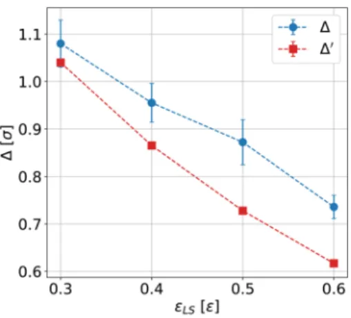
Figure 2presents the measured shifts between the wall surface and the HWP, Δ from fluid piston simulations using Eq.(4)and Δ′ from equilibrium simulations using Eq.(5), i.e., using the position of the GDP. Note that, even though Δ′ was measured from equi-librium simulations, we will still refer to it as the gravity-like flow hydrodynamic shift because Eq.(5)was derived analytically for a gravity-driven flow. In this figure, one can see that Δ′is comparable to Δ although they slightly differ for large εLS. In general, the
hydro-dynamic shifts for a pressure-driven and for a gravity-like flow do not have to be identical: indeed, while the pressure gradient and the gravity-like force identify in the bulk, they will generally differ in the molecular vicinity of the interface where the fluid becomes hetero-geneous. In particular, the gravity-like force distribution will follow that of the density and can result in a different effective BC for the bulk flow. InFig. 2, one can also see that, for both flows, the dis-tance between the wall surface and the HWP decreases with the wall wettability controlled by the εLSparameter (a higher εLScorresponds
to a more wettable system). We can understand this result in terms of GDP (Fig. 3): for a more wettable system, the peaks of the density
FIG. 2. Measured shifts between the wall surface and the HWP for different
inter-action strengthsεLSbetween liquid and solid particles. Blue circles:Δ from fluid
piston simulations using Eq.(4); red squares:Δ′from equilibrium simulations
using Eq.(5), i.e., using the position of the GDP.Δ and Δ′are similar (although
they differ slightly at highεLS); in particular, they both decrease for a higher wall
wettability.
J. Chem. Phys. 151, 041103 (2019); doi: 10.1063/1.5111966 151, 041103-3
FIG. 3. GDP representation (dashed blue line) of the liquid interfacial density profile
(full red line) for two differentεLS. The GDP is closer to the physical wall for a larger
εLSbecause of the stronger adsorption.
profile close to the wall are more pronounced, so the area of an effec-tive liquid with constant density is bigger, hence a larger value of h and a smaller value of Δ. We also varied εLL and found that its
impact was much smaller than that of εLS. This can be rationalized
based on the GDP. Indeed, changing εLLshould (at the first order)
rescale the whole liquid density profile so that the GDP should not change.
The results we obtained here for the HWP are significantly dif-ferent from the ones obtained by other studies5–7,17(with Δ between ∼1.1 and 2.5σ) and from the sometimes used assumption11,18 that Δ = 0σ. For the less wettable walls, the common assumption2,30,38–40 that Δ∼ 1σ agrees with our results. However, for higher εLS
val-ues, this assumption is generally not valid, especially in systems with significantly small slip lengths like the one discussed in this paper.
From the pressure-driven flow, in addition to the determina-tion of the HWP, one can also measure the system transport coef-ficients.Table Ireports the η and b results for a set of εLS
param-eters. Because the shear viscosity is a property of the bulk liquid and in all simulations the temperature and pressure are set con-stant, there is no effect of the wall wettability on η, and its value is comparable to the one obtained from Couette simulations. As ratio-nalized in previous work,49the slip length decreases with ε
LS: for a
less wettable system, the fluid friction coefficient is smaller which implies a higher value ofb = η/λ. If we compare these results with those obtained from Couette simulations, we can see that by means of the pressure-driven flow method, we obtained equivalentb and
η measurements with the same order of magnitude in the error
precision.
TABLE I. Shear viscosity η (in ετ/σ3) and slip length b (inσ) at T = 0.83ε/k
Band
p = 0.094ε/σ3, for different system wettabilities controlled byε
LS(inε): comparison
between fluid piston and Couette flow measurements.
Fluid piston Couette
εLS η b η b 0.3 1.422± 0.015 6.80± 0.10 1.409± 0.024 6.64± 0.25 0.4 1.421± 0.006 3.26± 0.02 1.414± 0.007 3.27± 0.09 0.5 1.428± 0.007 1.66± 0.08 1.412± 0.011 1.61± 0.08 0.6 1.417± 0.013 0.71± 0.08 1.410± 0.011 0.64± 0.07 CONCLUSION
We have shown that the position where the hydrodynamic BC imposed by walls should be applied can be efficiently deter-mined by measuring the wall shear stress in MD simulations of a Poiseuille flow. As a consequence, we have shown that for gravity-driven flows, the HWP is only controlled by the static density profile of the fluid close to the wall and identifies with the GDP, which can be measured from equilibrium simulations. Accordingly, the HWP could be estimated from previous work where the equilib-rium structure of liquid-solid interfaces was modeled.50 We then simulated a LJ fluid confined between two parallel frozen walls and measured the HWP by using a fluid piston to generate a pressure-driven flow. The pressure-pressure-driven flow hydrodynamic wall was com-parable (although not identical) to the GDP. We investigated the effect of wetting by varying the liquid-solid interaction energy. We found that the hydrodynamic BC applies in the liquid, at a dis-tance Δ from the wall surface varying from∼1σ (with σ the atomic diameter) on nonwetting walls to a fraction of σ on wetting walls. The decrease in Δ for increasing wetting can be rationalized in terms of GDP, which is shifted toward the solid when the adsorp-tion of the fluid increases on more wetting surfaces. The mea-sured values of Δ are generally lower than previous measures, which ranged between 1.1 and 2.5σ, but they correspond approximately to the standard assumption made in MD studies of liquid-solid slip that Δ∼ 1σ. Finally, we have shown that, in addition to the HWP, the Poiseuille flow simulation also provides an accurate esti-mate of the slip length and fluid viscosity by comparing the mea-sured values with those obtained from independent Couette flow simulations.
Overall, we have presented a simple, fast, and accurate method to fully characterize the transport properties of a confined fluid by measuring the viscosity, slip length, and HWP in a single Poiseuille flow simulation. Note that this method is not limited to the simple slab geometry considered here. For instance, it can easily be extended to cylindrical channels, where the wall shear stress is τw = fr/2, with f being the pressure gradient and r
being the hydrodynamic radius of the pore. The method should also apply to mixtures—for a gravity-like flow, one can show that Eqs. (5) and (6) apply when replacing the number of uid particles and the number density by the total mass of the liq-uid and the mass density, respectively—and to thermalized walls. We plan to investigate the latter case in the future. An analo-gous approach could also be applied to characterize the effec-tive wall position for interfacial heat transfer. We hope these results will help improve the characterization of the hydrody-namic BC by MD simulations in systems of interest for nanofluidic applications.
ACKNOWLEDGMENTS
This work was supported by the ANR, Project No. ANR-16-CE06-0004-01 NECtAR. T.O. and Y.Y. are supported by JSPS KAKENHI Grant Nos. JP18K03929 and JP18K03978, Japan, respec-tively. Y.Y. is also supported by JST CREST Grant No. JPMJCR18I1, Japan. L.J. is supported by the Institut Universitaire de France. L.J. benefited from a JSPS international fellowship for research in Japan.
The Journal
of Chemical Physics
COMMUNICATION scitation.org/journal/jcpREFERENCES
1L. Bocquet and E. Charlaix, “Nanofluidics, from bulk to interfaces,”Chem. Soc.
Rev.39, 1073–1095 (2010).
2
L. Bocquet and J.-L. Barrat, “Flow boundary conditions from nano- to micro-scales,”Soft Matter3, 685–693 (2007).
3C. Navier, “Mémoire sur les lois du mouvement des fluides,” Mem. Acad. Sci.
Inst. Fr. 6, 389 (1823).
4
B. Cross, C. Barraud, C. Picard, L. Léger, F. Restagno, and ˜A. Charlaix, “Wall slip of complex fluids: Interfacial friction versus slip length,”Phys. Rev. Fluids3, 062001 (2018).
5
L. Bocquet and J. L. Barrat, “Hydrodynamic boundary conditions, correlation functions, and Kubo relations for confined fluids,”Phys. Rev. E49, 3079–3092 (1994).
6C. J. Mundy, S. Balasubramanian, and M. L. Klein, “Hydrodynamic
bound-ary conditions for confined fluids via a nonequilibrium molecular dynamics simulation,”J. Chem. Phys.105, 3211–3214 (1996).
7C. J. Mundy, S. Balasubramanian, and M. L. Klein, “Computation of the
hydro-dynamic boundary parameters of a confined fluid via non-equilibrium molecular dynamics,”Physica A240, 305–314 (1997).
8
J. Delhommelle and P. T. Cummings, “Simulation of friction in nanoconfined fluids for an arbitrarily low shear rate,”Phys. Rev. B72, 172201 (2005).
9J. Petravic and P. Harrowell, “On the equilibrium calculation of the friction
coefficient for liquid slip against a wall,”J. Chem. Phys.127, 174706 (2007).
10
V. P. Sokhan and N. Quirke, “Slip coefficient in nanoscale pore flow,” Phys. Rev. E78, 015301 (2008).
11J. S. Hansen, B. D. Todd, and P. J. Daivis, “Prediction of fluid velocity slip at
solid surfaces,”Phys. Rev. E84, 016313 (2011).
12A. Bo¸tan, B. Rotenberg, V. Marry, P. Turq, and B. Noetinger, “Hydrodynamics
in clay nanopores,”J. Phys. Chem. C115, 16109–16115 (2011).
13
S. K. Kannam, B. D. Todd, J. S. Hansen, and P. J. Daivis, “Slip length of water on graphene: Limitations of non-equilibrium molecular dynamics simulations,” J. Chem. Phys.136, 024705 (2012).
14
S. K. Kannam, B. D. Todd, J. S. Hansen, and P. J. Daivis, “Interfacial slip friction at a fluid-solid cylindrical boundary,”J. Chem. Phys.136, 244704 (2012).
15
L. Bocquet and J.-L. Barrat, “On the Green-Kubo relationship for the liquid-solid friction coefficient,”J. Chem. Phys.139, 044704 (2013).
16K. Huang and I. Szlufarska, “Green-Kubo relation for friction at liquid-solid
interfaces,”Phys. Rev. E89, 032119 (2014).
17
S. Chen, H. Wang, T. Qian, and P. Sheng, “Determining hydrodynamic bound-ary conditions from equilibrium fluctuations,”Phys. Rev. E92, 043007 (2015).
18
B. Ramos-Alvarado, S. Kumar, and G. P. Peterson, “Hydrodynamic slip length as a surface property,”Phys. Rev. E93, 023101 (2016).
19A. Sam, R. Hartkamp, S. K. Kannam, and S. P. Sathian, “Prediction of fluid slip
in cylindrical nanopores using equilibrium molecular simulations,” Nanotechnol-ogy29, 485404 (2018).
20S. Nakaoka, Y. Yamaguchi, T. Omori, and L. Joly, “Extraction of the solid-liquid
friction coefficient between a water-methanol liquid mixture and a non-polar solid crystal surface by Green-Kubo equations,”Mech. Eng. Lett.3, 17–00422 (2017).
21
H. Nakano and S.-i. Sasa, “Statistical mechanical expressions of slip length,” J. Stat. Phys.176, 312 (2019).
22D. Camargo, J. A. de la Torre, R. Delgado-Buscalioni, F. Chejne, and P. Español,
“Boundary conditions derived from a microscopic theory of hydrodynamics near solids,”J. Chem. Phys.150, 144104 (2019).
23H. Nakano and S.-i. Sasa, “Microscopic determination of macroscopic boundary
conditions in Newtonian liquids,”Phys. Rev. E99, 013106 (2019).
24
P. A. Thompson and M. O. Robbins, “Shear flow near solids: Epitaxial order and flow boundary conditions,”Phys. Rev. A41, 6830–6837 (1990).
25
P. A. Thompson and S. M. Troian, “A general boundary condition for liquid flow at solid surfaces,”Nature389, 360–362 (1997).
26J. Barrat and L. Bocquet, “Influence of wetting properties on hydrodynamic
boundary conditions at a fluid/solid interface,”Faraday Discuss.112, 119–127 (1999).
27
M. Cieplak, J. Koplik, and J. R. Banavar, “Boundary conditions at a fluid-solid interface,”Phys. Rev. Lett.86, 803–806 (2001).
28K. Falk, F. Sedlmeier, L. Joly, R. R. Netz, and L. Bocquet, “Molecular origin
of fast water transport in carbon nanotube membranes: Superlubricity versus curvature dependent friction.”Nano Lett.10, 4067–4073 (2010).
29
S. K. Kannam, B. D. Todd, J. S. Hansen, and P. J. Daivis, “Slip flow in graphene nanochannels,”J. Chem. Phys.135, 144701 (2011).
30
S. K. Kannam, B. D. Todd, J. S. Hansen, and P. J. Daivis, “How fast does water flow in carbon nanotubes?,”J. Chem. Phys.138, 094701 (2013).
31S. K. Bhatia and D. Nicholson, “Friction between solids and adsorbed fluids is
spatially distributed at the nanoscale,”Langmuir29, 14519–14526 (2013).
32A. Botan, V. Marry, B. Rotenberg, P. Turq, and B. Noetinger, “How
elec-trostatics influences hydrodynamic boundary conditions: Poiseuille and electro-osmostic flows in clay nanopores,”J. Phys. Chem. C117, 978–985 (2013).
33
G. Tocci, L. Joly, and A. Michaelides, “Friction of water on graphene and hexag-onal boron nitride fromab initio methods: Very different slippage despite very similar interface structures,”Nano Lett.14, 6872–6877 (2014).
34L. Guo, S. Chen, and M. O. Robbins, “Slip boundary conditions over curved
surfaces,”Phys. Rev. E93, 013105 (2016).
35
S. Nakaoka, Y. Yamaguchi, T. Omori, and L. Joly, “Molecular dynamics analysis of the friction between a water-methanol liquid mixture and a non-polar solid crystal surface,”J. Chem. Phys.146, 174702 (2017).
36A. R. b. Saleman, H. K. Chilukoti, G. Kikugawa, M. Shibahara, and T. Ohara, “A
molecular dynamics study on the thermal energy transfer and momentum trans-fer at the solid-liquid interfaces between gold and sheared liquid alkanes,”Int. J. Therm. Sci.120, 273–288 (2017).
37M. P. Allen and D. J. Tildesley,Computer Simulation of Liquids, 2nd ed. (Oxford
University Press, 2017).
38
J. M. Georges, S. Millot, J. L. Loubet, and A. Tonck, “Drainage of thin liq-uid films between relatively smooth surfaces,”J. Chem. Phys.98, 7345–7360 (1993).
39T. Qian, X.-P. Wang, and P. Sheng, “Molecular scale contact line
hydrodynam-ics of immiscible flows,”Phys. Rev. E68, 016306 (2003).
40N. V. Priezjev and S. M. Troian, “Molecular origin and dynamic behavior of slip
in sheared polymer films,”Phys. Rev. Lett.92, 018302 (2004).
41P. Simonnin, V. Marry, B. Noetinger, C. Nieto-Draghi, and B. Rotenberg,
“Mineral- and ion-specific effects at clay–water interfaces: Structure, diffusion, and hydrodynamics,”J. Phys. Chem. C122, 18484–18492 (2018).
42
H. Hoang and G. Galliero, “Local viscosity of a fluid confined in a narrow pore,” Phys. Rev. E86, 021202 (2012).
43M. Morciano, M. Fasano, A. Nold, C. Braga, P. Yatsyshin, D. N. Sibley,
B. D. Goddard, E. Chiavazzo, P. Asinari, and S. Kalliadasis, “Nonequilibrium molecular dynamics simulations of nanoconfined fluids at solid-liquid interfaces,” J. Chem. Phys.146, 244507 (2017).
44I. Hanasaki and A. Nakatani, “Flow structure of water in carbon nanotubes:
Poiseuille type or plug-like?,”J. Chem. Phys.124, 144708 (2006).
45S. Plimpton, “Fast parallel algorithms for short—Range molecular dynamics,”
J. Comput. Phys.117, 1–19 (1995).
46
I. Hanasaki and A. Nakatani, “Fluidized piston model for molecular dynamics simulations of hydrodynamic flow,”Modell. Simul. Mater. Sci. Eng.14, S9–S20 (2006).
47J. A. Thomas, A. J. H. McGaughey, and O. Kuter-Arnebeck, “Pressure-driven
water flow through carbon nanotubes: Insights from molecular dynamics simula-tion,”Int. J. Therm. Sci.49, 281–289 (2010).
48
D. M. Heyes, “Shear thinning of the Lennard-Jones fluid by molecular dynam-ics,”Physica A133, 473–496 (1985).
49
D. M. Huang, C. Sendner, D. Horinek, R. R. Netz, and L. Bocquet, “Water slip-page versus contact angle: A quasiuniversal relationship,”Phys. Rev. Lett.101, 226101 (2008).
50
G. J. Wang and N. G. Hadjiconstantinou, “Molecular mechanics and struc-ture of the fluid-solid interface in simple fluids,”Phys. Rev. Fluids2, 094201 (2017).
J. Chem. Phys. 151, 041103 (2019); doi: 10.1063/1.5111966 151, 041103-5