Correlating Integrative Complexity With System Modularity
The MIT Faculty has made this article openly available.
Please share
how this access benefits you. Your story matters.
Citation
Sinha, Kaushik, Eun Suk Suh, and Olivier de Weck. "Correlating
Integrative Complexity With System Modularity." Proceedings of the
ASME 2017 International Design Engineering Technical Conferences
and Computers and Information in Engineering Conference IDETC/
CIE 2017, 6-9 August, 2017, Cleveland, Ohio, ASME, 2017, p.
V02AT03A048. © 2017 by ASME
As Published
http://dx.doi.org/10.1115/DETC2017-67254
Publisher
American Society of Mechanical Engineers
Version
Final published version
Citable link
http://hdl.handle.net/1721.1/115252
Terms of Use
Article is made available in accordance with the publisher's
policy and may be subject to US copyright law. Please refer to the
publisher's site for terms of use.
CORRELATING INTEGRATIVE COMPLEXITY WITH SYSTEM MODULARITY
Kaushik Sinha
Massachusetts Institute of Technology Cambridge, MA, USA
Eun Suk Suh*
Graduate School of Engineering Practice
Seoul National University Seoul, Korea
Olivier de Weck
Department of Aeronautics and Astronautics
Massachusetts Institute of Technology Cambridge, MA, USA
*Corresponding Author
ABSTRACT
Modularity is the degree to which a system is made up of relatively independent but interacting elements. Modularization is not necessarily a means of reducing intrinsic complexity of the system, but it is a means of effectively redistributing the total complexity across the system. High degree of modularization enable reductionist strategies of system development and is an effective mechanism for complexity re-distribution that can be better managed by system developers by enabling design encapsulation. In this paper, we introduce a complexity attribution framework to enable consistent complexity accounting and management procedure and show that integrative complexity has a strong inverse relationship with system modularity and its implication on complexity management for engineered system design and development.
1. INTRODUCTION
One of the fundamental tenets of system design is to keep the system architecture as simple as possible. However, contrary to basic design rules, architectures of latest engineering systems are becoming more complex due to ever-increasing complexity of new technologies and infrastructures to accommodate them. Engineering systems across domains have adopted significant technological and architectural changes to meet the forever increasing demand for higher performance. This has led to increased complexity and higher development effort in realizing such systems [1]. In a complex engineered system, multiple components and interfaces are designed together to perform one or more over-arching set of functions. The pattern of connections and their physical behavior cannot be thought of as truly regular or fully predictable. Understanding the system
behavior requires understanding of system elements and their pattern of connections [2]. This overall trend necessitates an important need for proper system architecture complexity management process. Without the smart complexity management, the system’s overall architecture may become unmanageable, leading to undesirable results, such as longer development period, higher R&D and lifecycle costs, and possible increase in system’s post-launch maintenance cost.
To better manage architectural arrangements of complex systems, one of the widely used system design strategy is modularization [3]. In modular design strategy, the system is decomposed into several sub-systems called modules. Modules have dense internal interactions, while having relatively few external connections to other modules. Until now, the literature efforts focused on solely measuring and managing system complexity, or system modularity in isolation with existing literature indicating that modularity and complexity are negatively correlated (i.e., higher modularity implying lower structural complexity) [3].
In this paper, we introduce the notion of integrative complexity and present preliminary observation that modularity index and integrative complexity, given any system decomposition, are negatively correlated. We provide statistical evidence that normalized integrative complexity can be used in lieu of modularity index for system modularity estimation.
2. LITERATURE REVIEW
Complexity and modularity are important inherent properties of complex engineering systems. As such, there has been a lot of works published in the subject of system complexity and modularity, and its implication to the overall complex system design. In the context of engineered system,
Proceedings of the ASME 2017 International Design Engineering Technical Conferences and Computers and Information in Engineering Conference IDETC/CIE 2017 August 6-9, 2017, Cleveland, Ohio, USA
complexity is defined as “the property of having many interrelated, interconnected, or interwoven elements and interfaces.” [4]. There are two main aspects of system complexity, which are internal complexity and external complexity. The internal complexity is closely related to overall system design, and is further divided into structural complexity, dynamic complexity, and organizational complexity [5, 6]. The external complexity is related to factors, which are not subject to control by system architects, such as market dynamics, political complexities and institutional complexities. The primary focus of this research is the distribution of internal-structural complexity of the engineered system, and the subsequent literature review is focused on published works in this particular area.
Structural complexity of a system is closely related to the complexity of individual system elements and degree of connectivity of the underlying system architecture. As result, the structural complexity has strong impact on the effort and cost of system design, development and operation [7-9]. Even though the primary goal of the system design organization is to optimize the overall cost related to the system being developed and operated by designing the system architecture as simple as possible, there is a need to incorporate essential complexity in the system to deliver the required level of system performance [4]. To this extent, the system architect, whose role is to create a balanced/optimal system architecture must balance the requirements between system design, development, and operation efforts, system performance, and the amount of complexity incorporated. In order to achieve this objective, one of the key task is to identify a suitable metric for measuring system complexity.
There are many complexity metrics proposed, with earlier works originating from the software engineering [10, 11]. Over time, several other metrics, based on different characteristics of the system, are introduced to academia. These include complexity metrics based on system element count-based measures [12-14], information and information transfer efficiency [15, 16], entity relationship graphs decomposition [17], hierarchy extension [5], network structure heterogeneity [18], empirical measure based on similar systems [19], and graph energy of the system [20]. Some of these developed metrics are used to assess the quantified value of complexity for various systems, including satellite systems [21], printing systems and basic architecture structure [22], aircraft engines [23, 24] and train undercarriage product platform [25] to name just a few.
Modularity refers to the property of a system where the system can be divided into different number of chunks called modules, which have strong intra-connections within individual module and weak interconnections between modules [3]. Modular design strategy refers to variety of methodologies that attempt to decompose complex systems into manageable modules, with each module typically performing a specific function required by the total system. In the context of complex system design, modular design strategies can be viewed as ways
to manage the inherent complexity by allocating them to individual modules. As with complexity, there has been many metrics proposed to measure system modularity.
According to Holtta-Otto et al. [26], modularity metrics are divided into two different types. The first type of metric measures the degree of coupling between modules, which is an indication of module independence. To this extent, several metrics were developed to measure the coupling density. Allen and Carlson-Skalak [27], Martin and Ishii [28], Newman [2], Sosa et al. [29], Guo and Gershenson [30], Holtta-Otto and de Weck [31], Whitfield et al. [32] and Jung and Simpson [33] proposed modularity metrics to measure the coupling density and demonstrated usefulness of their metrics on vehicle console, VCR cassette, jet engine, water cooler, camera, and computers. The second type of metrics identifies and measure similar features of modules, from the perspective of materials used, manufacturing process used, suppliers involved, and overall lifecycle issues. Proposed metrics by Newcomb et al. [34] and Gershenson et al. [35] are based on life cycle similarities. Siddique et al. [36] and Mikkola and Gassman [37] proposed modularity metrics that measured similarities in components, while Mattson and Magleby [38] proposed metrics measuring similarities in functions.
Parallel to defining various modularity measuring metrics, there have been works published that propose various modular design algorithms. Yu et al. [39] and Helmer et al. [40] proposed clustering algorithm based on Minimum Description Length (MDL) theory [41]. Van Beek et al. [42] proposed k-mean clustering algorithm based on modularity metric proposed by Whitfield [32]. Borjesson and Holtta-Otto [43] proposed clustering algorithms based on Module Function Deployment. Recently, Li et al. [44] proposed module partition methods based on directed and weighted networks. Others include Idicula-Gutierrez-Thebeau Algorithm (IGTA) [45], Cambridge Advanced Modeler [46], and community detection proposed by Blondel et al. [47].
In this paper, we propose an alternative approach for measuring system modularity that integrates two crucial aspects of complex system architecting, namely complexity and modularity, from complexity-centric viewpoint. This is done by introducing and developing the notion of integrative complexity and exploring its relationship to the degree of modularity for real-life complex systems. The work presented in this paper contributes to establish the relationship between structural complexity and the degree of system modularity and demonstrates that integrative complexity of the system can be used as a surrogate measure for system modularity.
In subsequent sections, we briefly introduce the method of complexity quantification, a complexity accounting process termed as complexity attribution, modularity metric and finally a detailed case study showing the application of this method to a train undercarriage system that leads to statistical validation of our claim that integrative complexity and modularity have strong negative correlation and it can be used as a surrogate for degree of modularity of the system.
3. PRIMER ON COMPLEXITY QUANTIFICATION AND COMPLEXITY ATTRIBUTION
3.1. Quantifying Complexity
There is a close relationship between the engineering system’s structural complexity and the “form” [4] of the system architecture, which depends on number of elements in the system, their characteristics and connectivity between system elements. The metric adopted to measure structural complexity [20, 23] in this paper captures complexity arising from (i) individual system elements; (ii) individual connections between system elements; and (iii) topology of connections for the overall system. Following is the mathematical expression of structural complexity metric for engineering systems, proposed by Sinha et al. [20, 23, 24].
1 2 3
Structural Complexity, CC C C Eq. (1) The overall structural complexity metric (C) shown in Eq. (1) is composed of three major terms. The first term (C1) is the total summation of individual element’s complexity. The second term (C2) is the summation of complexities arising from individual interaction between system elements. The last term (C3) represents the topological complexity of the system, resulting from the interface arrangements between elements in the system.
The first term (C1) captures individual element’s complexity, and does not contain any system architecture information. It can be re-written as sum of individual element’s complexity (i) as shown:
C1 i
i1 n
The second term (C2) is the sum of complexities of each pair-wise interaction, which is labeled as ij in the detailed representation of C2 below: C2 ijAij j1 n
i1 n
In the equation, A Mmn is the binary adjacency matrix which represents the connectivity structure of the system with following conditions: 1 [( , ) | ( ) and ( , ) ] 0 otherwise ij i j i j i j A
where represents the set of connected elements and n is the number of elements for the entire system.
Finally, the last term (C3) is the term that is directly related to the topological arrangements of system interfaces. In more detailed mathematical term, it is expressed as
C3E(A)
n , where E(A) i1
i(A) n
.In the equation, i(.) represents binary adjacency matrix A’s ith
singular value. The C3 term is very useful for quantifying topological complexity arising from different connectivity structure within the system. This term is also related to the effort required for system integration. One should also note that in order to calculate C3, it is required to have the overall knowledge of connectivity structure of the system, since it must be mapped to the adjacency matrix A. Using detailed terms introduced for C1, C2 and C3, the complexity metric in Eq. (1) can be rewritten as:
1 1 1 ( ) n n n i ij ij i i j E A C A n
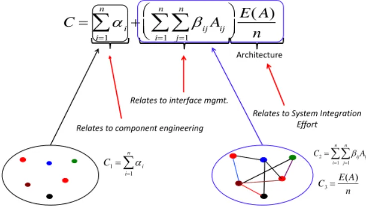
Eq. (2)Figure 1 shows terms shown in Eq. (2), with brief explanation of what each term represents. For more detailed explanation and mathematical proof, interested readers can refer to the work by Sinha [23]. C i i1 n
ij j1 n
i1 n
Aij E( A) n Architecture Relates to System Integration Effort Relates to component engineering Relates to interface mgmt. C1 i i1 n C2 ijAij j1 n i1 n C3 E(A) nFigure 1. Explanation of individual terms of the structural complexity metric
3.2. Complexity Attribution Method and System Decomposition
Complexity attribution is a method for consistent accounting of complexity assigned to different sub-systems/modules and contribution of complexity from system integration. In essence, the complexity attribution method describes how overall structural complexity is distributed within the system, given a system decomposition strategy. System decomposition strategy refers to the decomposition of any system into smaller sub-systems/modules that are easier to manage [47, 48]. There are
other related definitions or point of view on system decomposition [3] that often uses functional view of the system. Once system decomposition is made available, the complexity attribution process performs accounting of complexity of different modules and complexity due to integration of modules.
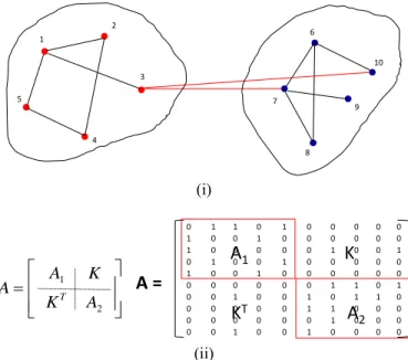
Let us define the system decomposition by a map Gr(.), which is an element to module map. Here each element is assigned to a module and this map is unique (i.e., an element can be a member of a unique module). It is probably best to use a motivating illustration in Fig. 2 as we move through the steps. In the figure we have a system with 10 elements and they are divided into two modules. The binary symmetric adjacency matrix A for this synthetic system representation can be written in terms of sub-matrices (A1, A2, K). Notice that sub-matrix K
represents the inter-module connectivity structure and is different from the number of modules, k with k = 2 in this case. Here A1 and A2 represent the binary adjacency matrices of
module 1 and 2 respectively.
10 1 2 3 4 5 6 7 8 9 (i) 0 1 1 0 1 0 0 0 0 0 1 0 0 1 0 0 0 0 0 0 1 0 0 0 0 0 1 0 0 1 0 1 0 0 1 0 0 0 0 0 1 0 0 1 0 0 0 0 0 0 0 0 0 0 0 0 1 1 0 1 0 0 1 0 0 1 0 1 1 0 0 0 0 0 0 1 1 0 0 0 0 0 0 0 0 0 1 0 0 0 0 0 1 0 0 1 0 0 0 0
A =
A
1A
2K
K
T A A1 K KT A2 (ii)Figure 2. (i) A hypothetical system composed of two modules, 10 elements and several bi-directional interfaces (ii) Simplified representation of a system in a Design Structure Matrix (DSM) form
Expanding to the general case with k modules and given system decomposition map Gr(.), we can express the individual module complexity for ith module as follows:
( ) ( ) ( ) ( )
1 2 3
i i i i
C C C C Eq. (3) where each term of the complexity metric are defined as
C
1 (i )
p (i ) p1 ni
; C
2(i )
pq (i ) q1 ni
p1 ni
A
pq (i ); C
3 (i )
E(A
(i))
n
i The method described is same as that of computing structural complexity metric for a module in isolation. Given the system decomposition, the integrative complexity is defined as( ) 1 k i i Integrative Complexity, IC C C
Eq. (4) Since the elements are divided into modules, we haveC1 C1(i )
i1 k
and therefore we can write integrative complexity (IC) as: ( ) ( ) 2 3 2 3 1 k i i iIC
C C
C C
Eq. (5)Hence, integrative complexity is independent of components and what matters are the interfaces and how they are topologically arranged. In order to compare different systems from multiple domains, it is helpful to use the normalized version of integrative complexity (ICn), defined as:
ICn 1 C2(i)C3(i) i1 k
C2C3 Eq. (6)Please note that the normalized integrative complexity is a ratio with ICn [0, 1] and therefore a dimensionless number.
As an illustrative example, let’s focus on the hypothetical system with two modules, shown in Fig. 2. For simplicity, let’s assume that all elements have unit complexity, i = 1, i and all interfaces have complexity ij = 0.1, i ≠ j. Each module has five elements and five within-module interfaces. Notice that while module 1 has only one module-bridging element (i.e., an element with interfaces across module boundary), module 2 has two module-bridging elements (namely elements 7 and 10). Applying the complexity quantification and attribution process to this hypothetical system, following result are obtained:
Table 1: Complexity quantification and attribution example based on hypothetical system shown in Fig. 2.
Term Value Description
C 11.49 Using Eqs. (1) and (2) C2*C3 1.49 Using Eq. (2)
C(i) {5.56,5.58} Using Eq. (3)
IC 0.35 Using Eq. (4) ICn 0.24 Using Eq. (6)
3.3. Modularity and System Decomposition
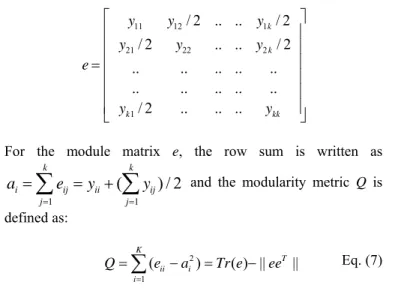
Now let’s focus our attention on modularity. Modularity estimation is based on the given system decomposition adopted and distribution of intra- and inter-module interfaces. Let’s define yii as fraction of intra-module interfaces while yij represents fraction of inter-module interfaces as defined in the nomenclature section. For computation of modularity index Q [2], a module matrix e (also known as community matrix) is constructed as: e y11 y12/ 2 .. .. y1k/ 2 y21/ 2 y22 .. .. y2 k/ 2 .. .. .. .. .. .. .. .. .. .. yk1/ 2 .. .. .. ykk
For the module matrix e, the row sum is written as
a
i
e
ij j1 k
y
ii (
y
ij j1 k
) / 2
and the modularity metric Q is defined as: 2 1 ( ) ( ) || || K T ii i i Q e a Tr e ee
Eq. (7) Here eii represents the fraction of edges with both end vertices in the same module i and ai is represents fraction of edges with at least one end vertex inside module i. To illustrate the process, consider the hypothetical system example shown in Fig. 2. In the example, module has five elements and five within-module interfaces. Module 1 has only one module-bridging element (element 3) while module 2 has two module-bridging elements (elements 7 and 10). Applying the method described above, we have: e 5 /12 1/12 1 /12 5 /12 a1 e11 e12 0.5 a2 e21 e22 0.5 Q e11 e22 [a12 a22] = 5/6-2(0.52) = 1/33.4. Relationship between Integrative Complexity and Modularity
As seen from Eq. (5), the integrative complexity is the part of overall structural complexity that excludes the module complexities. In other words, it is the complexity resulting from system integration (i.e., integration of modules as defined by the
system decomposition strategy) alone. The integrative complexity represents the part of structural complexity that arises due to integration of modules and therefore, does not include in-module complexity. For a given level of total complexity, a lower value of integrative complexity implies higher proportion of in-module complexity.
Although modularity is often construed to have strict negative correlation with system complexity, it is our hypothesis that there is exists a stronger relationship between modularity and integrative complexity. To demonstrate the validity of this hypothesis, a real-life complex engineering system was used. The analysis results of the example are presented in the next section.
4. TRAIN UNDERCARRIAGE EXAMPLE
In order to demonstrate the framework introduced in previous sections, a real-life complex system example was used. Figure 3 shows a train undercarriage model and the DSM of the undercarriage in its original decomposition configuration.
(a)
(b)
Figure 3. (a) Computer Aided Design (CAD) model of a train undercarriage (with permission from Korea Railroad Research Institute); (b) DSM of the train undercarriage
We applied different system decomposition strategies and observed the variation of normalized integrative complexity (ICn) and modularity index (Q) values. We generated a set of element-module maps (i.e., a table that maps each train undercarriage element to a unique module) for various system decomposition strategies. The suite of system decomposition strategies considered includes: (i) system decomposition adopted by the undercarriage system design team, (ii) multiple modularity maximization based decompositions techniques [2, 45, 47] and (iii) decompositions that result in optimal tradeoff between modularity and diversity of in-module complexity distribution. Note that decomposition technique described in [45] is stochastic in nature and produces different decompositions based on input parameter ranges. The community detection algorithm [47] also has stochastic characteristic associated to it, while Newman algorithm [2] is deterministic. Using these three system decomposition techniques, a subset of seven system decompositions all of which aims to maximize modularity with some differences in their decomposition paradigm are generated. Table 2 shows modularity index (Q) and normalized integrative complexity (ICn) values for generated decompositions.
Table 2. Value of Q and ICn and total number of modules
defined for train undercarriage under different system decomposition configurations Decomposition Q ICn #Modules 1 0.39 0.32 19 2 0.57 0.24 17 3 0.64 0.16 14 4 0.68 0.15 12 5 0.71 0.13 10 6 0.73 0.12 10 7 0.74 0.11 11
For this set of decompositions, we can observe that modularity index (Q) and normalized integrative complexity (ICn) shows strong negative correlation.
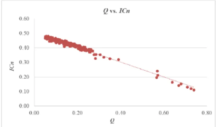
In order to investigate statistical significance of the correlation between Q and ICn, we require a much larger dataset for results to demonstrate any statistical significance. To accomplish this, the initial set of seven decompositions, suggested by approaches (i) – (iii) above, were augmented with random permutation of the existing seven decompositions to generate a dataset of 250 different system decompositions. The plot of Q and ICn values for generated decomposition configurations is shown in Fig. 4.
As we can observe from the figure, a vast majority of these randomly perturbed system decompositions happens to generate low system modularity with Q < 0.25 and are densely clustered around low modularity, high normalized integrative complexity regime of the distribution. Based on the dataset plot shown, analysis was performed to determine the statistical significance
between Q and ICn of given system decomposition. Results are shown in Table 3 and 4.
Figure 4. Linear relationship between Q and ICn for 250
different train undercarriage system decomposition configurations
Table 3. Statistical analysis results for Q vs. ICn plot shown
in Fig. 4
R2 R2
adj p-value Degree Of
Freedom
0.98 0.98 0.00 248
Table 4. Parameter values and associated statistic for Q vs.
ICn relationship for undercarriage system decompositions
(Linear model of the form: ICn = +*Q)
Coeffs Value ErrorStd. t-stat p-value Confidence
Interval
0.51 0.00 508.20 0.00 {0.50,0.51}
-0.51 0.00 -102.20 0.00 {-0.52,-0.50}
Results of this statistical analysis in terms of quality indicators (e.g., R2, p-value, t-statistics) and parameter
estimation shows a highly significant and stable linear relationship between Q and ICn.
From the results shown, we observe that Q and ICn have strong negative correlation that is statistically significant and lends credence to the use of integrative complexity as a surrogate for modularity. This result is not surprising since the notion of high modularity tends to emphasize higher in-module complexity and this leads to lower integrative complexity with a higher proportion of total complexity being embedded within modules. Therefore, integrative complexity and modularity are likely to be negatively correlated and this claim is substantiated through this case study.
5. CONCLUSIONS AND FUTURE WORK
We have presented a complexity attribution approach, based on complexity quantification methodology described in [23], to enable consistent complexity accounting process for effective complexity management across system representation levels (i.e., detailed representation to module-level) with explicit accounting for system integration using the newly introduced notion of integrative complexity. Systems are deemed to be more modular if they have lower integrative complexity.
Realized modularity is a function of system decomposition strategy adopted while system complexity is a system property and is independent of system decomposition strategy. Although total complexity and modularity may not show negative correlation, our study indicates integrative complexity and modularity are likely to show strong negative correlation and one might use one in lieu of the other.
The proposed complexity quantification and complexity attribution methods can be applied to any engineered complex systems that can be modeled as a network. In future, some insightful research based on results presented in this paper can be pursued further. One promising research topic is to perform the analysis presented to several complex systems across various domains and investigate whether the relationship between integrative complexity and modularity holds true, both within and across multiple domains of engineered complex systems. Another future research topic is a study to create a computational/virtual system architecting “sandbox” that will enable future studies on finding effective architectural patterns for specified contexts.
ACKNOWLEDGMENTS
This research was supported by the Basic Science Research Program through the National Research Foundation of Korea (NRF) funded by the Ministry of Education, Science and Technology (NRF-2016R1D1A1A09916273).
REFERENCES
[1] Arena, M. V., Younossi, O., Brancato, K., Blickstein, I., and Grammich, C. A., 2008, "Why has the cost of fixed-wing aircraft risen? A macroscopic examination of the trends in us military aircraft costs over the past several decades," DTIC Document.
[2] Newman, M. E. J., 2010, Networks : an introduction, Oxford University Press, Oxford ; New York.
[3] Baldwin, C. Y., and Clark, K. B., 2000, Design rules, MIT Press, Cambridge, Mass.
[4] Crawley, E., Cameron, B., and Selva, D., 2016, System architecture : strategy and product development for complex systems, Pearson, Boston.
[5] Lindemann, U., Maurer, M., and Braun, T., 2008, Structural complexity management: an approach for the field of product design, Springer Science & Business Media.
[6] Weber, C., 2005, "What is "Complexity"?," Proceedings ICED 05, the 15th International Conference on Engineering Design, Melbourne, Australia, 15.-18.
[7] Barton, J. A., Love, D. M., and Taylor, G. D., 2001, "Design determines 70% of cost? A review of implications for design evaluation," J Eng Design, 12(1), pp. 47-58.
[8] Braha, D., and Bar-Yam, Y., 2007, "The statistical mechanics of complex product development: Empirical and analytical results," Manage Sci, 53(7), pp. 1127-1145.
[9] Maier, M. W., and Rechtin, E., 2009, The art of systems architecting, CRC Press, Boca Raton.
[10] Kafura, D., and Henry, S., 1981, "Software Quality Metrics Based on Inter-Connectivity," J Syst Software, 2(2), pp. 121-131.
[11] McCabe, T. J., 1976, "A complexity measure," Ieee T Software Eng(4), pp. 308-320.
[12] Bralla, J. G., 1986, Handbook of product design for manufacturing : a practical guide to low-cost production, McGraw-Hill, New York.
[13] Pahl, G., and Beitz, W., 1996, Engineering design : a systematic approach, Springer, London ; New York.
[14] Whitney, D. E., Dong, Q., Judson, J., and Mascoli, G., "Introducing knowledge-based engineering into an interconnected product development process," Proc. Proceedings of the 1999 ASME Design Engineering Technical Conferences.
[15] Allaire, D., He, Q. X., Deyst, J., and Willcox, K., 2012, "An Information-Theoretic Metric of System Complexity With Application to Engineering System Design," J Mech Design, 134(10).
[16] Kortler, S., Kreimeyer, M., and Lindemann, U., "A planarity-based complexity metric," Proc. DS 58-6: Proceedings of ICED 09, the 17th International Conference on Engineering Design, Vol. 6, Design Methods and Tools (pt. 2), Palo Alto, CA, USA, 24.-27.08. 2009.
[17] Ameri, F., Summers, J., Mocko, G., and Porter, M., 2008, "Engineering design complexity: an investigation of methods and measures," Res Eng Des, 19(2-3), pp. 161-179.
[18] Dehmer, M., 2011, Structural analysis of complex networks, Birkhäuser, Dordrecht ; New York.
[19] Bearden, D. A., 2003, "A complexity-based risk assessment of low-cost planetary missions: when is a mission too fast and too cheap?," Acta Astronaut, 52(2-6), pp. 371-379.
[20] Sinha, K., and de Weck, O. L., 2013, "A network-based structural complexity metric for engineered complex systems," Systems Conference , 2013 IEEE International, IEEE, pp. 426-430.
[21] Tamaskar, S., Neema, K., and DeLaurentis, D., 2014, "Framework for measuring complexity of aerospace systems," Res Eng Des, 25(2), pp. 125-137.
[22] Min, G., Suh, E. S., and Holtta-Otto, K., 2016, "System Architecture, Level of Decomposition, and Structural Complexity: Analysis and Observations," J Mech Design, 138(2).
[23] Sinha, K., 2014, "Structural complexity and its implications for design of cyber-physical systems," Massachusetts Institute of Technology.
[24] Sinha, K., Shougarian, N. R., and de Weck, O. L., 2017, "Complexity Management for Engineered Systems Using System Value Definition," Complex Systems Design & Management, Springer, pp. 155-170.
[25] Kim, G., Kwon, Y., Suh, E. S., and Ahn, J., 2016, "Analysis of Architectural Complexity for Product Family and Platform," J Mech Design, 138(7).
[26] Holtta-Otto, K., Chiriac, N. A., Lysy, D., and Suh, E. S., 2012, "Comparative analysis of coupling modularity metrics," J Eng Design, 23(10-11), pp. 787-803.
[27] Allen, K. R., and Carlson-Skalak, S., "Defining product architecture during conceptual design," Proc. 1998 ASME Design Engineering Technical Conference, Atlanta, GA. [28] Martin, M. V., and Ishii, K., 2002, "Design for variety: developing standardized and modularized product platform architectures," Research in Engineering Design-Theory Applications and Concurrent Engineering, 13(4), pp. 213-235. [29] Sosa, M. E., Eppinger, S. D., and Rowles, C. M., 2007, "A network approach to define modularity of components in complex products," J Mech Design, 129(11), pp. 1118-1129. [30] Guo, F., and Gershenson, J. K., "A comparison of modular product design methods based on improvement and iteration," Proc. ASME 2004 International Design Engineering Technical Conferences and Computers and Information in Engineering Conference, American Society of Mechanical Engineers, pp. 261-269.
[31] Holtta-Otto, K., and de Weck, O., 2007, "Degree of modularity in engineering systems and products with technical and business constraints," Concurrent Eng-Res A, 15(2), pp. 113-126.
[32] Whitfield, R. I., Smith, J. S., and Duffy, A. B., "Identifying component modules," Proc. Artificial Intelligence in Design’02, Springer, pp. 571-592.
[33] Jung, S., and Simpson, T. W., 2017, "New modularity indices for modularity assessment and clustering of product architecture," J Eng Design, 28(1), pp. 1-22.
[34] Newcomb, P. J., Bras, B., and Rosen, D. W., 1998, "Implications of modularity on product design for the life cycle," J Mech Design, 120(3), pp. 483-490.
[35] Gershenson, J. K., Prasad, G. J., and Allamneni, S., 1999, "Modular product design: a life-cycle view," Journal of Integrated Design and Process Science, 3(4), pp. 13-26.
[36] Siddique, Z., Rosen, D. W., and Wang, N., "On the applicability of product variety design concepts to automotive platform commonality," Proc. ASME Design Engineering Technical Conferences.
[37] Mikkola, J. H., and Gassmann, O., 2003, "Managing modularity of product architectures: Toward an integrated theory," Ieee T Eng Manage, 50(2), pp. 204-218.
[38] Mattson, C. A., and Magleby, S. P., "The influence of product modularity during concept selection of consumer products," pp. 9-12.
[39] Yu, T. L., Yassine, A. A., and Goldberg, D. E., 2007, "An information theoretic method for developing modular architectures using genetic algorithms," Res Eng Des, 18(2), pp. 91-109.
[40] Helmer, R., Yassine, A., and Meier, C., 2010, "Systematic module and interface definition using component design structure matrix," J Eng Design, 21(6), pp. 647-675.
[41] Rissanen, J., 1999, "Hypothesis selection and testing by the MDL principle," Comput J, 42(4), pp. 260-269.
[42] Van Beek, T. J., Erden, M. S., and Tomiyama, T., 2010, "Modular design of mechatronic systems with function modeling," Mechatronics, 20(8), pp. 850-863.
[43] Borjesson, F., and Holtta-Otto, K., 2014, "A module generation algorithm for product architecture based on component interactions and strategic drivers," Res Eng Des, 25(1), pp. 31-51.
[44] Li, Y., Wang, Z., Zhang, L., Chu, X., and Xue, D., 2017, "Function Module Partition for Complex Products and Systems Based on Weighted and Directed Complex Networks," J Mech Design, 139(2), pp. 021101-021101.
[45] Sharman, D. M., 2002, "Valuing Architecture For Strategic Purposes, unpublished M. Sc," thesis, MIT, Cambridge, MA. [46] Wynn, D. C., 2007, "Model-based approaches to support process improvement in complex product development," University of Cambridge.
[47] Blondel, V. D., Guillaume, J. L., Lambiotte, R., and Lefebvre, E., 2008, "Fast unfolding of communities in large networks," J Stat Mech-Theory E.
[48] Ulrich, K. T., and Eppinger, S. D., 2012, Product design and development, McGraw-Hill/Irwin, New York.