The MIT Faculty has made this article openly available. Please share
how this access benefits you. Your story matters.
Citation Pierson, Kawika, and John D. Sterman. “Cyclical Dynamics of Airline
Industry Earnings.” Syst. Dyn. Rev. 29, no. 3 (July 2013): 129–156.
As Published http://dx.doi.org/10.1002/sdr.1501
Publisher Wiley Blackwell
Version Author's final manuscript
Citable link http://hdl.handle.net/1721.1/88125
Terms of Use Creative Commons Attribution-Noncommercial-Share Alike
Cyclical Dynamics of Airline Industry Earnings
Kawika Pierson*
Atkinson Graduate School of Management, Willamette University, Salem OR
John Sterman
MIT Sloan School of Management, Cambridge, MA
ABSTRACT
Aggregate airline industry earnings have exhibited large amplitude cyclical behavior since deregulation in 1978. To explore the causes of these cycles we develop a behavioral dynamic model of the airline industry with endogenous capacity expansion, demand, pricing, and other feedbacks; and model several strategies industry actors have employed in efforts to mitigate the cycle. We estimate model parameters by maximum likelihood methods during both partial model tests and full model estimation using Markov chain Monte Carlo methods to establish confidence intervals. Contrary to prior work we find that the delay in aircraft acquisition (the supply line of capacity on order) is not a very influential determinant of the profit cycle. Instead we find that aggressive use of yield management—varying prices to ensure high load factors (capacity utilization)—may have the unintended effect of increasing earnings variance by increasing the sensitivity of profit to changes in demand.
KEYWORDS: Earnings cycles, Profit cycles, Airlines, Operational leverage, Capacity supply line, Yield management
* Corresponding author: [email protected]
Introduction
Researchers in system dynamics have studied cyclicality in industries and the economy for decades (Forrester, 1961; Meadows, 1970; Mass, 1975), and have generally concluded that profit cycles are caused by a failure to fully account for delays in the negative feedbacks controlling inventory, capacity acquisition, or other resources. Unfortunately, the low salience of capacity on order (Sterman, 1989; Sterman, 2000) together with long capacity lifetimes and high fixed costs often limit the implementation of strategies to mitigate the cycle, because managers can be reluctant to accept that such important decisions could have been detrimental (Ghaffarzadegan and Tajrishi, 2010; Goncalves, 2003).
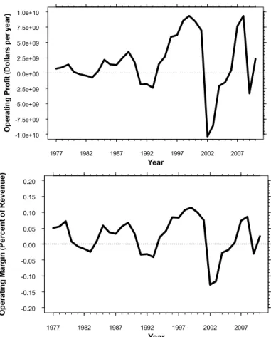
Figure 1: US airline industry operating profit and operating margin (profit/revenue)
Since deregulation in 1978 aggregate earnings of the US airline industry have fluctuated with an average peak-‐to-‐peak period of approximately ten years and a long run mean very close to zero (Hansman and Jiang, 2005), as shown in Figure 1. The amplitude of the cycle in profit margin (operating profit/revenue, a scale-‐free measure of profit fluctuations), has not diminished in the 35 years since deregulation. In this paper we build a model of the airline industry that examines the origin of the cycle. Airline industry cyclicality has been
Op e ra tin g P ro fit ( D o lla rs p e r y e a r) Year -1.0e+10 -7.5e+09 -5.0e+09 -2.5e+09 0.0e+00 2.5e+09 5.0e+09 7.5e+09 1.0e+10 1977 1982 1987 1992 1997 2002 2007 Op e ra tin g M a rg in ( P e rc e n t o f R e v e n u e ) Year -0.20 -0.15 -0.10 -0.05 0.00 0.05 0.10 0.15 0.20 1977 1982 1987 1992 1997 2002 2007
addressed in the system dynamics literature (Liehr et al., 2001; Lyneis, 2000), but we expand the boundary of these models1 to include an endogenous account of feedbacks omitted from some earlier work, including price setting, wages, and air travel demand. Including these feedbacks allows us to more closely represent the structure of the industry so as to better test policies designed to moderate the cycle. The model also includes structures representing yield management, mothballing, and ancillary revenues (e.g., baggage check fees) to address how existing strategic decisions influence profits and profit variability.
The airline industry is an excellent setting for research on profit cycles. The government requires airlines to report detailed information about their operations, and makes these data available to the public. By avoiding proprietary sources of data, we provide a fully documented model that scholars and industry professionals can use to better understand the dynamics of earnings cycles in general. We estimate model parameters via maximum likelihood methods, using both partial model tests (Homer, 2012) and full model estimation, and show how standard errors can be estimated efficiently in multivariate system dynamics models using Markov chain Monte Carlo methods.
Airlines are also advantageous as a research setting because of their importance. The Federal Aviation Administration (2011) estimates that commercial aviation contributes $1.2 to $1.3 trillion per year to the economy and generates between 9.7 and 10.5 million jobs in the US. Yet despite the importance of the industry, consistent profitability has been elusive. Industry analysts and experts are not blind to this pattern of behavior. Like their peers in other cyclical industries, they consistently argue either that specific events were the cause of the cycle turning points (e.g., recessions or terrorist attacks) or that new strategies will dampen the cycle in the future (Doganis, 2002). These arguments persist in the face of a history of strategies, such as mergers, leasing, yield management, and mothballing that have failed to stabilize aggregate profits.2
Consistent with prior system dynamics work, we find that the cycle arises from delays in negative feedbacks involving the mutual regulation of demand, capacity, load factor (capacity utilization), and prices. Unlike prior work, we find evidence that the cycle in capacity is strongly moderated by airline pricing policies, specifically the use of yield management, which increases the responsiveness of prices to variations in demand relative to capacity and boosts average load factors. However, sensitivity tests varying the strength of the yield management feedback suggest that in the aggregate, airline pricing decision rules increase operational leverage and the variance in profitability, and may place the industry near a global minimum of the risk-‐return space.
1 Lyneis (2000) has a similar model boundary but is proprietary.
2Yield, the industry term for dollars per revenue passenger mile, and price are used interchangeably in this paper. Yield management is the process of “finding the optimal tradeoff between average price paid and capacity utilization” (Weatherford and Bodily, 1992).
Model simulations, together with the low average price to earnings ratio of airline stocks and the high incidence and cost of airline bankruptcies, suggest that airlines could potentially improve long-‐run shareholder value by adopting policies that pursue less vigorous yield management. The feasibility and full impacts of such policies for individual airlines may depend on competitive dynamics beyond the level of aggregation of the model however, so we close by discussing the limitations of our analysis and suggestions for future research to build on the results here.
Model Structure
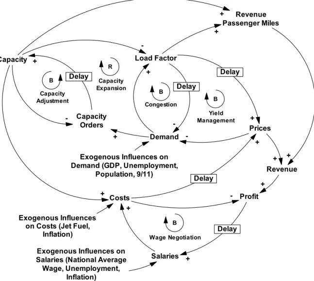
Figure 2 shows a high level causal diagram summarizing the principal feedbacks captured by and the exogenous influences to the model.
Figure 2: Overview of the model feedback structure and boundary. Capacity Costs Prices Demand Profit Revenue + + -+ + + + Load Factor -+ Salaries + + Exogenous Influences on Demand (GDP, Unemployment, Population, 9/11) -Exogenous Influences on Salaries (National Average
Wage, Unemployment, Inflation)
-Exogenous Influences on Costs (Jet Fuel,
Inflation) B Yield Management B Congestion B Wage Negotiation R Capacity Expansion Capacity Orders + -B Capacity Adjustment Revenue Passenger Miles + + + Delay Delay Delay Delay Delay
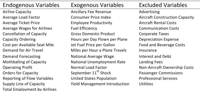
Table 1 provides a summary of the model boundary, listing the main endogenous, exogenous and excluded variables.
Endogenous Variables
Exogenous Variables
Excluded Variables
Airline Capacity Ancillary Fee Revenue Advertising
Average Load Factor Consumer Price Index Aircraft Construction Capacity
Average Ticket Price Employee Productivity Aircraft Rental Costs
Average Wages for Airlines Fuel Efficiency Communication Costs
Cancellation of Capacity Gross Domestic Product Corporate Taxes
Capacity Ordering Hours per Day Flown per Plane Depreciation Expense
Cost per Available Seat Mile Jet Fuel Price per Gallon Food and Beverage Costs Demand for Air Travel Miles per Hour a Plane Travels Insurance
Demand Forecasting National Average Wage Interest and Debt
Mothballing of Capacity National Unemployment Rate Landing Fees
Operating Profit Normal Load Factor Non-‐Aircraft Ownership Costs
Orders for Capacity September 11th Shock Passenger Commissions
Reporting of Flow Variables United States Population Professional Services
Supply Line of Capacity Yield Management Introduction Utilities
Total Employment by Airlines
Table 1: Model boundary diagram highlighting the most important endogenous, exogenous and excluded variables in the model. To the extent that excluded expenses vary with inflation they are indirectly represented in the model.
The model is organized into four principal sectors: Capacity, Demand, Prices and Costs. Here we describe the formulations for several critical variables. The online supplement (OS4) contains full model documentation using SDM-‐Doc (Martinez-‐Moyano, 2012) and all model, simulation, and experimentation documentation requirements (Rahmandad and Sterman, 2012).
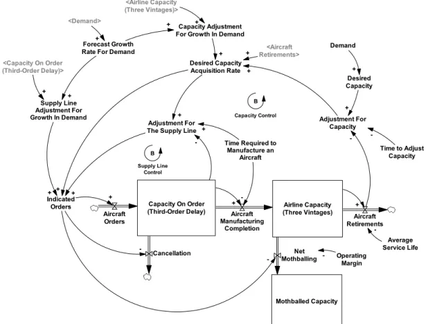
Aggregate airline capacity is reported in available seat-‐miles per year. Each seat is assumed to fly a constant average number of miles per year determined from historical data for aircraft utilization. Airline capacity, the number of seats in the fleet, is modeled with a modified version of the standard stock control structure in the system dynamics literature (Sterman, 2000, Ch. 17). The stock of aircraft in service (Figure 3) is disaggregated into three vintages, with a mean aircraft lifetime of thirty years. The aircraft acquisition delay is assumed to be third order, with a mean acquisition time of two years (Airbus, 1998). Airlines are assumed to place orders to replace retirements of old aircraft and adjust capacity to demand given the normal load factor, while accounting for the supply line of aircraft on order, any returning to service from mothballing, and the expected rate of growth in demand (eq. 1 through 5):
DCA = R + CA!+ (DC − C)/τ! (2)
SLA = (DCA ∗ τ! − SL)/τ! (3)
SLA!= S ∙ w ∙ !! (4)
CA! = C ∙ w ∙ !! (5)
Aircraft orders are the sum of desired capacity acquisition (DCA), the supply line adjustment (SLA), and the two growth adjustments (CAg and SLAg), less capacity returning
to service from the stock of mothballed aircraft (RS). DCA is the sum of retirements (R), CAg, and a capacity adjustment based on the difference between desired capacity (DC)
and current capacity (C). The strength of that capacity adjustment is controlled by τ!, the
estimated time to adjust capacity. Similarly, the supply line adjustment, SLA, is the gap between the desired and actual supply line, divided by the supply line adjustment time, τ!.
The desired supply line is determined, following Little’s Law, by the product of the desired capacity adjustment, DCA, and the delay in manufacturing a plane (τ!).
Figure 3: Overview of capacity and capacity acquisition.
Capacity On Order
(Third-Order Delay) (Three Vintages)Airline Capacity Aircraft Orders Aircraft Manufacturing Completion Aircraft Retirements Mothballed Capacity Net Mothballing Adjustment For Capacity -Time to Adjust Capacity -Desired Capacity + Demand + Adjustment For The Supply Line -Indicated Orders + + Supply Line Control B Capacity Control B Time Required to Manufacture an Aircraft + Desired Capacity Acquisition Rate + <Aircraft Retirements> + Operating Margin -+ + Capacity Adjustment For Growth In Demand
+
+
Cancellation + Forecast Growth
Rate For Demand
<Airline Capacity (Three Vintages)> + + Supply Line Adjustment For Growth In Demand + + Average Service Life -<Capacity On Order (Third-Order Delay)> + <Demand> +
We assume that airlines may plan for the growth of air travel demand. The growth adjustments, CAg and SLAg, increase orders based on ge, the expected fractional growth
rate in demand, with a weight, w, representing the extent to which the airlines actually account for the growth in demand when ordering capacity. The growth adjustments assure that under constant exponential growth there is no steady state error (if w = 1). A proof is available in the online supplement (OS2). The expected rate of growth is based on past growth rates using a standard trend function (Sterman, 2000, ch. 16).
Demand for air travel is modeled as depending on population and air travel demand per capita. Population is exogenous. Per capita air travel demand depends on GDP per capita, the national unemployment rate, ticket prices, congestion, and an exogenous shock that captures the impact of the 9/11 terrorist attacks.
Demand = !!∙ Pop ∙ E!"#∙ E!"#$%∙ E!"#$%∙ E!"#$∙ E!/!! (6)
Air travel demand rises with growing incomes (Schafer, 1998), with an income elasticity
!!"# to be estimated:
E!"# =
GDP per capita Reference GDP per Capita
!!"#
(7)
Unemployment is a common independent variable in regressions used to forecast air travel demand, even when income effects are also included (Carson et al., 2011). We normalize unemployment by its historical average as shown below:
E!"#$%= 1 − Unemployment Rate 1 − Reference Unemployment !!" (8)
The unemployment rate is exogenous.
The effects of air travel prices and system congestion, measured by load factor, are: E!"#$%= Price Price!"# !!" (9)
E!"#$= !"##$ℎ Perceived Load Factor
Normal Load Factor , τcon
!!"
(10)
SPD is the price elasticity of demand, and reference price is the initial ticket price, scaled by
inflation. The normal load factor has changed over the last 40 years with improvements in system operations and information technology. We model the reference load factor as
the best-‐fit quadratic for historical load factor3, and SCD is the sensitivity of demand to
congestion. There is a delay in the public’s perception of congestion, so perceived load factor is modeled by first order smoothing. Since there is also a delay before congestion changes flying habits the ratio of perceived to normal load factor is smoothed again, with an adjustment time τcon.
The terrorist attacks of September 11th 2001 immediately reduced air travel
demand, with an effect that lingered for several years. The details of this formulation can be found in the online supplement (OS4).
Ticket prices are modeled with a standard price-‐discovery, hill-‐climbing formulation (Sterman, 2000, Ch. 13). Current ticket prices adjust with a delay to the indicated ticket price, which anchors on the current price and adjusts to pressures from profit margins, costs, and load factor:
Price = Price!"#− Price
τ! + P0 (11)
Price!"# = Price ∙ E!"#$∙ E!" (12)
E!"#$ =
Expected Passenger Cost ∙ (1 + Target Profit Margin)
Price (13)
Expected Passenger Cost
= Total Costs-‐Ancillary Fees
Available Seat Miles*Normal Load Factor
(14)
E!" =
Load Factor Normal Load Factor
!!"#
(15)
Airlines in the model calculate their expected costs per passenger, on a seat mile basis, using current costs less any fees collected. Net cost is divided by the expected passenger volume, given by capacity and the normal load factor, to yield the expected cost per seat-‐ mile, which is then marked up by the target profit margin. Total operating costs are the sum of costs from wages, costs from fuel, and other costs. Both fuel prices and fuel efficiency are exogenous. Other costs are modeled as an initial dollar amount per seat mile that grows with the Consumer Price Index.
Airline ticket prices also respond to imbalances between demand and supply, as indicated by load factor (Kimes, 1989). At the level of an individual carrier low load factors indicate that prices for the flight in question should fall. In the short term this will increase demand for that flight, and for the individual firm. Naturally, however, firm-‐level
3The quadratic approximation for normal load factor fits well over the period from 1970 to 2010, with an R2
of 95.6%. The regression estimates are statistically significant at the 1% level. Omitting the quadratic term significantly degrades the endogenous model’s fit for demand.
demand elasticity is much higher than industry-‐level demand elasticity (Oum et al., 1990), so most of the increase in the individual carrier’s load factor comes at the expense of their rivals, who will respond with similar fare reductions. In the aggregate this causes prices to fall when load factors are low and rise when planes are relatively full. This relationship is captured in Equation 15.
While most yield management research is focused on pricing at the level of individual firms, in industry-‐level models such as the one developed here it is necessary to model the evolution of industry average prices, a common practice in system dynamics, including Meadows’ (1970) commodity cycle model, Mass’ (1975) business cycle model, Forrester’s National Model (Forrester, 1979), many models of the oil industry (e.g., Davidsen et al., 1990), shipping industry (e.g., Randers and Göluke, 2007), electric utility industry (e.g. Ford, 1997), and others, including prior airline industry models (Liehr et al., 2001; Lyneis, 2000).
When yield management technology was introduced to the airline industry in 1985 ticket prices became much more responsive to load factor (Smith et al., 1992). To capture this effect the sensitivity of prices to the supply demand balance, SSDP, is modeled as a
step increase in 1985, the size of which is estimated during model calibration.
To model average airline employee wages we again employ a standard hill-‐ climbing formulation in which wages respond to three pressures: profit margin, unemployment, and outside opportunities (wages in other industries). If there were no net effect from these pressures the average wage would increase with inflation.
Wage = Wage!"#− Wage
τ! + W0 (16)
where τW is the delay in adjusting wages, and W0 is the initial average wage.
Wage!"# = Wage ∙ E!"#$%&∙ E!"#$%∙ E!""∙ (1 + ∆CPI) (17)
Industry profitability is reported with a delay because it takes time for the parties in collective bargaining negotiations (airlines and unions) to form expectations about profits from past data. Wages tend to rise when airlines are relatively profitable and fall when they are less profitable:
E!"#$%& = 1 + Margin!"# 1 + Margin!"# !!" (18)
The reference margin in Equation 18 is the historical average margin for the industry, calculated from the data. The perceived margin, MarginPer, is modeled using first order
exponential smoothing of operating profit margin, with a delay time to be estimated, along with the strength of the effect of profitability on wage negotiations, SMW.
We model normal unemployment as the average historical value over the horizon of the model: E!"#$% = Unemployment Normal Unemployment !!" (19)
Wages should also respond to wages in other industries. Since there is a skill premium offered for jobs in the airline industry, average airline wages are higher than the national mean. We assume airline wages respond to the national average wage (NAvgWage) adjusted by the average wage premium, with a sensitivity to be estimated.
E!"" = Wage
NAvg Wage*Wage Premium !!"
(20)
Consistent with the literature in system dynamics (e.g. Sterman, 2000), and the broader literature in behavioral decision making and cognitive psychology (e.g. Stanovich, 2011), the decision rules for pricing, wages, aircraft orders, mothballing, etc., are boundedly-‐ rational, behavioral heuristics, grounded in well-‐established evidence regarding the way managers make decisions in complex dynamic systems.
The online supplement (OS4) provides full documentation of the model.
Airline Industry Data
The data for parameter estimation come from the Air Transport Association (ATA), the nation's oldest and largest airline trade association, the Bureau of Transportation Statistics (BTS), and MIT's Airline Data Project (ADP).4 These data include available seat miles (capacity), revenue passenger miles (demand), average ticket price per revenue passenger mile (price), average wage per worker, including salary, benefits and other compensation (wage), and aggregate operating profit (profit). Data for U.S. population comes from the Census Bureau, while GDP data for the U.S. are from the Bureau of Economic Analysis and measured in real, year 2000 dollars per capita. The CPI, national average wage, and unemployment data come from the Bureau of Labor Statistics. Jet fuel prices per gallon and employee productivity are obtained from the ATA. Ancillary fees come from the ADP.
Parameter Estimation
We estimated model parameters by minimizing the weighted sum of the squared error between the model and the data simultaneously for each of the relevant data series:
4ATA: www.airlines.org; ADP: http://web.mit.edu/airlinedata/www/default.html. The ATA is now known as Airlines for America.
min!∈R ! !"− !!" ! !! !=0 MSE(!!) ! !=0 (21)
where the data series !i include historical demand, prices, wages, operating profit, etc.,
depending on the particular partial model test or full model estimation performed. The error from each series is weighted by the root mean square error of the model estimate from the previous calibration run. The process is iterated until the weights and estimates converge.
The sum of squared errors for each variable included in the estimation process is weighted by the reciprocal of the root mean squared error between the simulated and actual data series. Doing so assures, assuming normally distributed errors, that the total estimation error will be distributed chi-‐square, allowing us to estimate confidence intervals for each parameter using a Markov chain Monte Carlo (MCMC) method (Gelman et al., 2003). We use MCMC to simulate the distribution of the log likelihood payoff surface given joint changes in the parameters. The MCMC algorithm was implemented using commercially available software and we provide a detailed description in the appendix (A2). Convergence took approximately 1.2 million model runs, or close to 16 hours of desktop computer time.
Partial model testing (Homer, 2012) was the first stage of our parameter estimation process. Each sector of the model was isolated and driven by historical data for the inputs to that sector. In the partial model test of the demand formulation (eq. 6), we use historical ticket prices and load factor rather than their endogenous values, along with historical GDP, unemployment, and population, to estimate demand. The partial model test for growth expectations uses historic demand to fit the trend function for expected growth in demand (an input to the capacity decision) against ten years of FAA demand forecasts. The partial model test of industry capacity replaced endogenous demand and profit with historical demand and operating profit. The partial model test for costs used historical wages and capacity together with exogenous fuel costs, efficiency, and inflation. The partial model test for industry wages used historical operating profit along with national unemployment, average wage, and inflation. The partial model test for price setting used historical operating costs, demand and capacity instead of their endogenous formulations.
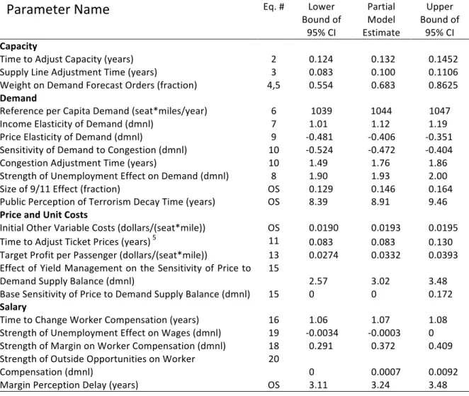
The estimated parameters from partial model testing are reported in Table 2, along with the 95% confidence intervals estimated by the MCMC method. Figure 4 compares the simulated and actual data for the partial model tests, and Table 3 reports goodness of fit measures. Overall the partial model tests have low error as a percentage of the mean and low bias, as shown by the Theil inequality statistics, indicating the errors are generally unsystematic.
The estimated parameters in the partial model tests are reasonable. The structure for the impact of the 9/11 terrorist attacks captures an immediate decline in air travel,
and the subsequent reduction in demand due to fear and the resulting security measures, which is assumed to gradually decrease over time. The estimated parameters suggest an immediate drop of nearly 15% in demand and a decay time of approximately 9 years. Sensitivity tests involving first order delays, higher order delays, and other specifications for the effect of 9/11 on demand all showed time constants on the order of the one reported here. The long decay time suggests the impacts of 9/11 have been persistent, perhaps a result of later, failed attacks such as the shoe and underwear bombers, or the inconvenience and costs of the security measures implemented since 2001. Alternatively, it is possible that some other factors caused a shift in the demand for air travel after 2001.
Parameter Name
Eq. # Lower Bound of 95% CI Partial Model Estimate Upper Bound of 95% CI CapacityTime to Adjust Capacity (years) 2 0.124 0.132 0.1452
Supply Line Adjustment Time (years) 3 0.083 0.100 0.1106
Weight on Demand Forecast Orders (fraction) 4,5 0.554 0.683 0.8625
Demand
Reference per Capita Demand (seat*miles/year) 6 1039 1044 1047
Income Elasticity of Demand (dmnl) 7 1.01 1.12 1.19
Price Elasticity of Demand (dmnl) 9 -‐0.481 -‐0.406 -‐0.351
Sensitivity of Demand to Congestion (dmnl) 10 -‐0.524 -‐0.472 -‐0.404
Congestion Adjustment Time (years) 10 1.49 1.76 1.86
Strength of Unemployment Effect on Demand (dmnl) 8 1.90 1.93 2.00
Size of 9/11 Effect (fraction) OS 0.129 0.146 0.164
Public Perception of Terrorism Decay Time (years) OS 8.39 8.91 9.46
Price and Unit Costs
Initial Other Variable Costs (dollars/(seat*mile)) OS 0.0190 0.0193 0.0195
Time to Adjust Ticket Prices (years) 5 11 0.083 0.083 0.130
Target Profit per Passenger (dollars/(seat*mile)) 13 0.0274 0.0332 0.0393
Effect of Yield Management on the Sensitivity of Price to
Demand Supply Balance (dmnl) 15 2.57 3.02 3.48
Base Sensitivity of Price to Demand Supply Balance (dmnl) 15 0 0 0.172
Salary
Time to Change Worker Compensation (years) 16 1.06 1.07 1.08
Strength of Unemployment Effect on Wages (dmnl) 19 -‐0.0034 -‐0.0003 0
Strength of Margin on Worker Compensation (dmnl) 18 0.291 0.372 0.409
Strength of Outside Opportunities on Worker
Compensation (dmnl) 20 0 0.0007 0.0092
Margin Perception Delay (years) OS 3.11 3.24 3.48
Table 2: Estimated parameters from partial model testing, with Markov chain Monte Carlo 95% confidence intervals. The equation number “OS” indicates that the equation is reported in the online supplement (OS4), not in the paper.
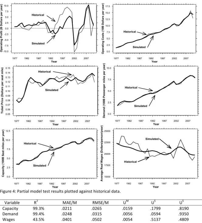
Figure 4: Partial model test results plotted against historical data.
Variable R2 MAE/M RMSE/M UM US US
Capacity 99.3% .0211 .0265 .0159 .1799 .8190
Demand 99.4% .0248 .0315 .0056 .0594 .9350
Wages 43.5% .0401 .0502 .0054 .5137 .4809
Cost 99.6% .0260 .0368 .0708 .0574 .8718
Prices 86.4% .0398 .0481 .0079 .0075 .9846
Profit 56.4% N/A N/A .0011 .1799 .8190
Table 3: Partial model fits to historical data for 1977-‐2010. R2 is defined as one minus the ratio of the sum of
the squared error to the total sum of squares. MAE/M is mean absolute error divided by the mean of the data. RMSE/M is the root mean square error divided by the mean of the data. Um, Us, and Uc are the Theil inequality statistics (Sterman, 2000, ch. 21), which partition the MSE into the fraction arising from bias (unequal means of simulated and actual data), unequal variances, and unequal covariation, respectively. MAE/M and RMSE/M are not reported for profit because average historical profit is very close to 0.
Op er at in g P ro fit ( B D o lla rs p er y ea r) Year -10.0 -7.5 -5.0 -2.5 0.0 2.5 5.0 7.5 10.0 1977 1982 1987 1992 1997 2002 2007 Historical Simulated Op er at in g C o st s ( 10 B D o lla rs p er y ea r) Year 0.0 2.5 5.0 7.5 10.0 12.5 15.0 17.5 1977 1982 1987 1992 1997 2002 2007 Historical Simulated Ti ck et P ri ce ( D ol la rs pe r se at m il e) Year 0.05 0.06 0.07 0.08 0.09 0.10 0.11 0.12 0.13 0.14 0.15 1977 1982 1987 1992 1997 2002 2007 Historical Simulated De m an d ( 10 0B P as se n g er m il es p er y ea r) Year 0.0 2.5 5.0 7.5 10.0 1977 1982 1987 1992 1997 2002 2007 Historical Simulated Ca p ac it y (1 00 B S ea t m il es p er y ea r) Year 0.0 2.5 5.0 7.5 10.0 12.5 1977 1982 1987 1992 1997 2002 2007 Historical Simulated Av e ra g e Re a l W a g e s ( Do lla rs /p e rs o n /y e a r) Year 15000 17500 20000 22500 25000 1977 1982 1987 1992 1997 2002 2007 Historical Simulated
The partial model tests indicate that the model reproduces sector-‐level behavior quite well, with the exception of the average airline industry wage. The fit of the model to the wage data is somewhat lower than the fit to the other variables. However, the mean absolute error is only 4% of the average of the historical wage data and the bias is very small. The fit of the model to the data, including the fit for wages, compares favorably against other models in the system dynamics literature and in related modeling traditions such as the forecasting literature. For example, Makridakis et al. (1982) examined the performance of a wide range of forecasting and modeling methods, using data from a large variety of systems. Typical calibration errors (assessed by the mean absolute percentage error, MAPE), for a subsample of 111 data series, were about 20% for non-‐ seasonal methods applied to the raw data, about 11% for methods that accounted for seasonal adjustments, and about 9% for the non-‐seasonal methods applied to the seasonally adjusted data.
Nevertheless, additional research into the determinants of airline wages would help to address the source of the unexplained variation in airline wages and whether these sources are plausibly endogenous or reflect factors unrelated to the cycle in aggregate profitability. For example, industry wages may be heavily influenced by bankruptcies of individual carriers and labor actions such as strikes, both of which are difficult to predict and not modeled here.
The partial model tests examine the ability of individual formulations to replicate industry dynamics given the actual, realized values of the inputs to each formulation or decision. However, the partial model tests cut important feedbacks in the system, so it is also necessary to examine the ability of the full, endogenous model to fit the data.
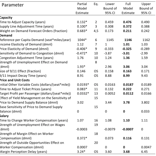
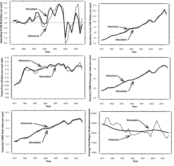
Full model estimation results (Tables 4, 5; Figure 5) improve the fit for demand, price, and operating profit compared to the partial model results. The fit for the other variables remains similar. All series show low bias and, with the exception of wages, low unequal variation. The estimated parameters are plausible and the MCMC confidence bounds generally tight. The estimated values of a number of parameters are very similar to the values in the partial model tests, for example, the size and decay time of the 9/11 effect. Several others, however, differ from the partial model estimates.
In particular, in the full system estimation the capacity sector of the model became significantly less reactive, with longer time constants for capacity and supply line adjustment, and a smaller response to demand forecasts. In the partial model test for capacity acquisition the time constant controlling the adjustment for the supply line was 0.1 years, suggesting that airlines are keenly aware of and swiftly adjust the supply line of aircraft on order as the desired number of aircraft they seek to acquire changes. Evidence from experimental studies (e.g. Sterman, 1989; Aramburo et al., 2012; Croson et al., forthcoming), and from other industries (e.g., commercial real estate and shipbuilding, see Sterman, 2000; Randers and Göluke, 2007) suggests weak supply line adjustment and a role for inadequate supply line control in the genesis of industry cycles. However, the high price of aircraft, concentrated nature of the industry, and contractual terms for aircraft orders may favor fully accounting for the supply line. The supply line adjustment time in
the full model estimation is longer and more plausible, though at about 4 months, still short enough to suggest that airlines are quite sensitive to the supply line of capacity on order. Exploring this issue further would require data on order cancellations, aircraft completion, and the supply line of planes, perhaps at the level of individual manufacturers, data that are not publicly available.
Parameter
Partial Model Estimate Eq. Lower Bound of 95% CI Full Model Estimate Upper Bound of 95% CI CapacityTime to Adjust Capacity (years) 0.132* 2 0.459 0.476 0.490
Supply Line Adjustment Time (years) 0.100* 3 0.308 0.372 0.388
Weight on Demand Forecast Orders (fraction) 0.683* 4,5 0.173 0.211 0.242
Demand
Reference per Capita Demand (seat*miles/year) 1044* 6 1145 1146 1162
Income Elasticity of Demand (dmnl) 1.12 7 1 1.01 1.03
Price Elasticity of Demand (dmnl) -‐0.406* 9 -‐0.333 -‐0.325 -‐0.289
Sensitivity of Demand to Congestion (dmnl) -‐0.472* 10 -‐3.87 -‐3.01 -‐2.99
Congestion Adjustment Time (years) 1.76 10 1.24 1.36 1.59
Strength of Unemployment Effect on Demand
(dmnl) 1.93* 8 2.96 3.06 3.04
Size of 9/11 Effect (fraction) 0.146 OS 0.158 0.163 0.171
9/11 Impact Decay Time (years) 8.91 OS 8.88 8.99 9.43
Price and Unit Costs
Initial Other Variable Costs (dollars/(seat*mile)) 0.0193* OS 0.0163 0.0187 0.0189
Time to Adjust Ticket Prices (years) 0.083* 11 0.132 0.222 0.271
Target Profit per Passenger (dollars/(seat*mile)) 0.0332* 13 0.0052 0.0112 0.0166 Effect of Yield Management on the Sensitivity of
Price to Demand Supply Balance (dmnl) 3.02 15 3.44 3.78 3.802
Base Sensitivity of Price to Demand Supply
Balance (dmnl) 0
15
0 0 0.033
Salary
Time to Change Worker Compensation (years) 1.07 16 1.08 1.10 1.11
Strength of Unemployment Effect on Wages
(dmnl) -‐0.0003
19
-‐0.0079 -‐0.0007 0 Strength of Margin Effect on Worker
Compensation (dmnl) 0.372* 18 0.073 0.116 0.131
Strength of Outside Opportunities Effect on
Worker Compensation (dmnl) 0.0007 20 0 0 0.0047
Margin Perception Delay (years) 3.24* OS 3.60 3.68 6.45
Table 4: Estimated parameters from full model results, with Markov chain Monte Carlo 95% confidence intervals, and partial model parameters for comparison. Partial model estimates marked with an asterisk (*) are statistically significantly different from the full model estimates at the 5% level.
Figure 5: Full model results plotted against the historical data.
Variable R2 MAE/M RMSE/M UM US US
Capacity 99.4% .0207 .0249 .0011 .0557 .9432
Demand 99.8% .0148 .0179 .0010 .0008 .9981
Wages 50.83% .0407 .0497 .0098 .6257 .3645
Cost 99.6% .0278 .0360 .0852 .0331 .8818
Prices 90.76% .0300 .0384 .0176 .0304 .9520
Profit 62.8% N/A N/A .0085 .0894 .9021
Table 5: Goodness of fit for full model, 1977-‐2010.
What accounts for the differences in parameter estimates between the partial and full models? First, the payoffs are different: in the partial model tests, the payoff is the fit to the focal variable in each sector: demand for the demand sector, capacity for the capacity sector, total cost for the cost sector and so on. In the full model estimation, the likelihood function is the sum of squared errors for all the key variables, specifically, demand,
Op e ra tin g P ro fit ( B D o lla rs p e r y e a r) Year -10.0 -7.5 -5.0 -2.5 0.0 2.5 5.0 7.5 10.0 1977 1982 1987 1992 1997 2002 2007 Simulated Historical Op e ra tin g C o s ts ( 1 0 B D o lla rs p e r y e a r) Year 0.0 2.5 5.0 7.5 10.0 12.5 15.0 17.5 1977 1982 1987 1992 1997 2002 2007 Historical Simulated Ti c k e t P ri c e ( D ol la rs pe r s e a t m ile ) Year 0.05 0.06 0.07 0.08 0.09 0.10 0.11 0.12 0.13 0.14 0.15 1977 1982 1987 1992 1997 2002 2007 Historical Simulated De m a n d ( 1 0 0 B P a s s e n g e r m ile s p e r y e a r) Year 0.0 2.5 5.0 7.5 10.0 1977 1982 1987 1992 1997 2002 2007 Historical Simulated Ca p a c it y ( 1 0 0 B S e a t m ile s p e r y e a r) Year 0.0 2.5 5.0 7.5 10.0 12.5 1977 1982 1987 1992 1997 2002 2007 Historical Simulated Av e ra g e Re a l W a g e s ( Do lla rs /p e rs o n /y e a r) Year 15000 17500 20000 22500 25000 1977 1982 1987 1992 1997 2002 2007 Historical Simulated
capacity, prices, profits, and average wages, weighted by 1/RMSE for each. Second, the likelihood function for the full model appears to have a flat optimum. Over one million MCMC runs were needed to arrive at stable estimates for the confidence bounds. Further, to prevent convergence to local optima we used multiple starting points in the parameter space. Many of these restarts discovered unique local maxima, indicating that the global likelihood surface is relatively flat over the range of plausible values. Recent work on parameter testing and model validation (Hadjis, 2011; Groesser and Schwaninger, 2012) use relatively simple models to advocate for particular approaches to parameter identification, estimation and model testing. The airline industry context however, like many policy relevant settings, involves common and troublesome issues arising from endogeneity, collinearity, under-‐identification, and flat optima, rendering these approaches potentially problematic and indicating a need for more research.
Model Analysis
Oscillations in dynamic systems arise from negative feedbacks with significant phase lag elements (time delays). System dynamics models of earnings cyclicality have found that delays in the negative feedbacks controlling inventory, capacity acquisition or other resources are the underlying causes of cyclical movements in the economy and for many industries and commodities (e.g., Meadows, 1969; Chen et al., 2000; Sterman, 2000, chs. 17, 19 and 20; and Randers and Goluke, 2007). Unsurprisingly, our results are consistent with this mechanism: delays in the negative feedbacks regulating airline industry capacity as demand and profitability change contribute to the oscillation observed in industry profitability. However, many prior studies find that the amplitude and persistence of industry cycles are increased by the failure of industry participants to account sufficiently for the supply line of capacity on order. The failure to account for the supply line is well supported by experimental, econometric, and field evidence (e.g., Sterman, 1989; Sterman, 2000, Ch. 17; Randers and Goluke, 2007), and previous models of the airline industry (Liehr et al., 2001) also highlight the role of the supply line in profit instability. However, supply line adjustment is only one of many delayed negative feedbacks in the airline industry. Our estimation results provide little evidence for failure to account for the supply line of aircraft on order as a source of the cycle in airline industry profitability. If industry participants, particularly the aircraft manufacturers, were unresponsive to the supply line of unfilled orders, then the estimated time constant for supply line adjustment would be very long, and longer than the capacity adjustment time. Instead, the supply line adjustment time we estimate is about the same as the capacity adjustment time in both the partial and full model tests. The result is plausible compared to, say, the real estate industry, where evidence suggests very low salience and responsiveness to the supply line (Sterman, 2000, Ch. 17.4.3). The real estate market is characterized by many producers, low barriers to entry, and therefore low experience among developers, and heterogeneity in building location, quality and price. It also is difficult to measure the supply line in real estate since it includes potential projects and
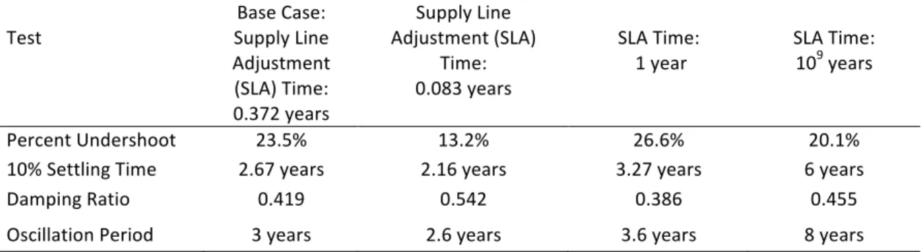
![[PDF] formation d introduction à l'Algorithmique et programmation gratuit | Cours informatique](data:image/gif;base64,R0lGODlhAQABAIAAAP///wAAACH5BAEAAAAALAAAAAABAAEAAAICRAEAOw==)