Costs of implementation: Bargaining
costs versus allocative efficiency
The MIT Faculty has made this article openly available. Please share
how this access benefits you. Your story matters.
Citation Maciejovsky, Boris, and Birger Wernerfelt. “Costs of
Implementation: Bargaining Costs Versus Allocative Efficiency.” Journal of Economic Behavior & Organization 77, no. 3 (March 2011): 318–325.
As Published http://dx.doi.org/10.1016/j.jebo.2010.11.004
Publisher Elsevier
Version Author's final manuscript
Citable link http://hdl.handle.net/1721.1/107903
Terms of Use Creative Commons Attribution-NonCommercial-NoDerivs License
COSTS OF IMPLEMENTATION: BARGAINING COSTS VERSUS ALLOCATIVE EFFICIENCY by Boris Maciejovsky and Birger Wernerfelt* May 7, 2009 *
MIT Sloan School of Management, Cambridge, MA, [email protected] [email protected].
Comments from David Budescu, Robert Gibbons, Werner Gueth, Oliver Hart, Teck Ho, Muhamet Yildiz, Christian Zehnder, and workshop participants at MIT and Harvard are gratefully acknowledged. Of course, the usual disclaimer applies.
A mechanism with low directcost of use may be preferredto alternatives implementing more efficient allocations. We show this experimentally by giving pairs of subjects the
option to agree on a single average price for a sequence of trades –in effect pooling several small bargains into a larger one. We makepooling costly by tying it to some inefficient trades, but subjects nevertheless reveal strong tendencies to pool, particularly when more bargains remain to be struck andwhen bargaining is face to face.The results
suggest thatimplementation costs could play a significant role in the use of many common trading practices, including the employment relationship.
COSTS OF IMPLEMENTATION: BARGAINING COSTS VERSUS ALLOCATIVE EFFICIENCY
The original literature on comparative economic systems evaluatesmechanisms in terms of their ability to implement efficient allocations as well asthe costs ofrequired
activities, such as information gathering, communication, and bargaining (e.,g. Hayek, 1945; Hurwicz, 1959). Yet, the latter class of costs plays almost no role in modern
thinking on mechanism and market design. Challenging this practice, we provide experimental evidence, showing that players trade-off efficiency for costs by accepting less efficient allocations in exchange for fewer rounds of bargaining.
In our studies,subjects havethe option to agree on a single average price for a
sequence of small trades –in effect pooling several bargains into one. The experiments
impose no artificial bargaining costs;subjects’ only gain from pooling is to reduce the amount of bargaining they have to do. In spite of this, many pairs of subjects agree to pool, even at the cost of completing some inefficient trades. The tendency to pool is stronger when the associated allocative inefficiencies are smaller, when more rounds of bargaining are “saved”, and when bargaining is face-to-face. On the other hand, the time
saved by pooling does not appear to be a significant factor. Agreements on pooling prices are preceded by a larger number of offers and counter-offers than agreements on
individual prices. Part of this is due to the fact that pairs who eventually choose to pool make more offers than pairs who never pool, even when negotiating individual prices.
Beyond suggesting that bargaining costs are positive, a more specific implication
of our results is that these costs are sub-additive (since subjects prefer tobargain over a single pooled price rather than over a sequence of individual prices).Sub-additivity has
strongintuitive appealand is consistent with the sense that most peoplewould prefer to
negotiate a single $300 deal instead of thirty $10 deals.
Sub-additive bargainingcosts areto bargaining what menucosts (Mankiw, 1985; Levy et al., 1997; Zbaracki et al. 2004)are to posted prices. They can help us explain the
widely observedpracticeof using a single price for any element in relatively large sets of heterogeneous items: college tuition typically does not depend on courses taken, haircuts
can be “as you like it”, and stays at all-inclusive resorts can take many forms. While these practices have been largely ignored by economists, the US Supreme Court has defended
them as rational responses to sub-additive pricing costs (Broadcast Music Inc. vs. Columbia Broadcast System, 1978). The American Society of Composers, Authors and
Publishers,which license the work of individual artists in the music industry, charges a blanket fee to bars, radio stations, etc. When the Columbia Broadcast System challenged
this practice, the court found in favor of the defendant,arguing that “…a blanket license
was an obvious necessity if the thousands of individual negotiations, a virtual
impossibility, were to be avoided.” Wernerfelt (1997) used similar arguments to explain
the absence of ongoing bargaining between employees and their bosses.1 Our
experimentsspeak directly to this by testingthe extent to which subjects are willing to
forego surplus in order to avoid ongoing bargaining.
The remainder of the paper is organized as follows: We present a reduced form model in Section II, the experimental design in Section III, and the results in Section IV. The paper closes with abrief discussion in Section V. The experimental instructions can
be found in anAppendix along with a possible micro-foundation for the model and some
more detailed data.
To demonstrate the existence and sub-additivity of bargaining costs, we will derive somegeneral conditions under which bargainers will preferto pool a set of
bargains.To keep the exposition as simple as possible, we will use a reduced form model
of sequential bargaining. A possible foundation for this reduced form is analyzed in
AppendixI.
We index a particular gameby where is the total number of
gamesthe subjects can play. The seller’s costs and the buyer’s valuation are I.I.D.
draws from two differentiable distributions, and , respectively. Expected gains from
trade are ( - , and theexpected magnitude of positive gains from trade is ?? (
1The author went further and contrasted the employment relationship with independent
contracting based on whether the agreement gives the bu yer control over production methods. “A contract on finished goods gives the bu yer no right to ask for different production methods as long as the product
specifications are met. The supplier is responsible only for “what” is done, not for “how”, and he is [thus] not an employee.” (p. 500).So an agreement to pool is an emplo yment relationship if the scope of the agreement is broad enough to include different production methods. Whether or not this is considered a satisfactory rationale for the existence of firms, it explains a prominent aspect of behavior within them.
II. A REDUCED FORM MODEL
n = 1, 2, …N, N
cn vn
Fc Fv
G = ??v c) dFvdFc
The analysis of the last game (game )is straightforward. If the gains from trade are positive, both players have positive expected payoffs. Following the above, these
payoffssum to – , where = 0 are bargaining costs. If the gains from trade are negative, the players will immediately agree not to tradeand the payoffssum to zero.
Considerthe next to last gameunder the assumption that the players engage in sequential bargaining. If gains from trade are positive, payoffs sum to – , where = 0, and if the gains from trade are negative, payoffs sum to zero. Since contracting is sequential, the expected payoffs from the last two games are – + – Suppose insteadthat the players decide to pool the last two games. The expected payoffs
from the current game are – , where are the bargaining costs associated with agreeing on the pooled contract The sub-additivity of bargaining costs is captured by the assumption that - + Since pooling commits the players to trade in the last game, the expected payoffs from that are . So pooling is preferable if
– + – = – + . Given that bargaining costsare sub-additive, we can work backwards to see that pooling becomes less and less attractive as more periods go by. In sum, gives the following
We test this proposition in a series of comparisons, involving sevenexperimental
treatments.
Two hundred and twenty-four students, 101 women and 123males, aged 18 to 51
years (M=23.16, SD=4.29), participated in the experiment, which was conducted at the Computer Lab for Experimental Research (CLER) at Harvard Business School,the
Behavioral Research Lab at the Massachusetts Institute of Technology,the University of
Vienna, Austria, and the Max Planck Institute of Economics, Germany. Experimental sessions lasted between 40 and 50 m inutes, and participants earned, on average, $15.04 (SD=2.49), including a show-up fee of $10.
N vN–cN bN bN vN-1–cN-1 bN-1 bN-1 vN-1–cN-1 bN-1 G+ bN. vN-1–cN-1 pN-1 pN-1 . pN-1 [bN 1, bN bN-1). G vN-1–cN-1 bN-1 G+ bN vN-1–cN-1 pN-1 G (1) (1)
: Pooling is more attractivewhen morebargaining costs are saved, whenfewer inefficient trades are included, and when more periods remain.
Î
Proposition
Upon arrival in the lab, subjectswere randomly assigned to dyads. Within each dyad, one of the subjects was assigned the role of a buyer, the other the role of a seller. Participants bargained over fictitious commodities over several bargaining games via a computer interface (see details below). Participants received written instructions (see AppendixII), and were asked to complete a short quiz that tested their understanding of the instructions. The experiment started only after all participants had answered all the quiz items correctly.
In order to be as conservative as possible, we donot impose any artificial bargaining costs,therebyallowingsubjects to reveal their ‘true’ preferences.Several
important classes of bargaining costs are thus absent, including inefficiencies resulting from lingering negative sentiments (Hart and Moore, 2008)and costs incurred during
attempts to gather pre-bargaining intelligence about the opponent’s reservation price.3 The only costs relevant to the experiment are those incurred during the bargaining
process itself. These are out-of-equilibrium costs in some models (Rubinstein, 1982), but not in all (Watson, 1998; Smith and Stacchetti, 2003; Dewatripont and Tirole, 2005). In
this paper, we will attemptto identify some factors bearing on the magnitude and nature of these bargaining costs.
At the beginning of each bargaining game, valuations for buyers and costs for sellers were randomly drawn from uniform distributions, which were common
knowledge to both parties. On top of that, subjectshadcomplete information in each
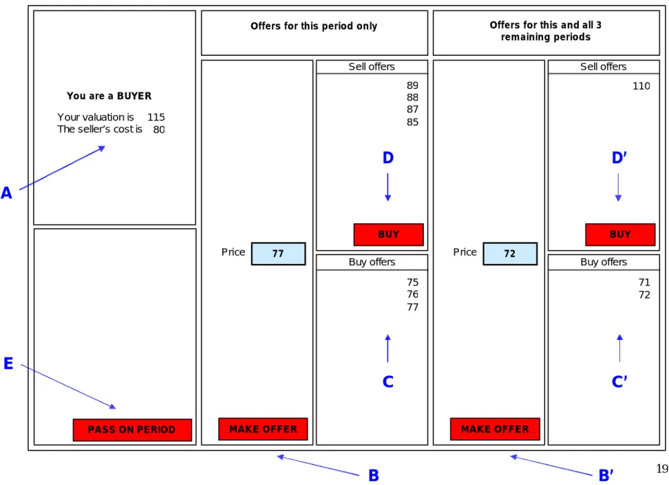
game about the realized valuations and costs of both buyers and sellers(see Ain Figure
1). Time is continuous, allowing either player to make an offer (bid or ask) at any time (regardless of who made the previous offer). To allow for the pooling of bargains,
participantscouldsubmit their own offers for the current bargaining game only(see B)
and/or for the current plus all remaining games (see B’). These offers were publicly listed
(see C and C’). Alternatively, participants could accept standing bargaining offers(D and
2
See Camerer (2003) for an overview of experimental studies of bargaining.
3Since better
-informed bargainers achieve better results (Busse, Silva-Risso, and Zettelmeyer, 2006), it is rational to invest in information search in anticipation of bargaining (Wernerfelt, 2008).
Similarly, players may refrain from suggesting improved trades in order to withhold information about such
opportunities to protect their own future bargaining power (Simester and Knez, 2002). A survey by found that purchasing managers spend 25% of their time “Preparing bids” and “Researching Prices”.
2
D’).Finally, the recipient of a bid/ask could accept it, make a counter-offer, wait for a
better offer, or unilaterally abort the current game (thus moving the pair to the next game,
see E).
For example,in Figure 1, the buyer submitted offers for the current game of 75, 76, and 77 Experimental Currency Units (ECU)4, and offers for the current and all remaining games of 71 and 72 ECU. The most attractive (since lowest) standing offer was 85 ECU for the current game and 110 ECU for the current plus all remaining games.
Participants’ profits were the difference between the valuation and the accepted price for buyers and the difference between the accepted price and the costs forsellers. If
participants passed on a game, the profits of both parties were zero for that particular
game.
[Insert Figure 1 about here]
We run sevenstudies in which we manipulate the inefficiency cost entailed by
pooling, the number of games, and the anonymity of bargaining. In each study, 16 dyads
of buyers and sellers bargain over fictitious items (see Appendix IIfor detailed
instructions).
Study 1: Existence and sub-additivity
The existence,and sub–additivity, of bargaining costs is tested in all the studies,
and also in the first, whichserves as the base treatment (BT) for later comparisons. In
BT, subjects bargain over 30 games with some inefficient trades.5Buyers’valuations are drawn from a uniform distribution ranging from 95 to 135 ECU, and sellers’ costs from a uniform distribution ranging from 65 to 105 ECU. In this treatment,trade is efficient with
4
One ECU was equivalent to 1 Cent in five of our seven treatments and equivalent to 6 Cents in
two treatments. 5
In order to maximize the intended similarity with the emplo yment situation, players remained with their partner throughout. A drawback of this is that we have to wave our hand at repeated game arguments. However, these could be avoided by re-shuffling all continuing (non-pooling) players after each
round.
probability 31/32. If only efficient trades are made, expected gains per game are 30.1,
whereasthey are 30 if all trades are made. So the expected cost of pooling is 3, or about
.33% of total surplus. We thus expect pooling by pairs for which the savings in bargaining costsare above 3 ECU.
The purpose of the next two studies is to check the validity of the bargaining cost interpretation by seeing if the extent of pooling varies withthe costs in terms of
inefficient trades.
Study 2: High costs of pooling
Inthe second study, the inefficient treatment (IT), we increase the costs of
pooling by includingmore inefficient trades. In IT, subjects bargain again over 30 games. Buyers’ valuations are drawn from a uniform distribution ranging from 90 to 140 ECU, and sellers’ costs from a uniform distribution ranging from 60 to 110 ECU. So in this
treatment, trade is efficient with probability 23/25. If only efficient trades are made,
expected gains per period are 30.53, whereasthey are 30 if all trades are made. The
expected cost of pooling is 15.99, or about 1.78 % of total surplus. We thusexpect that fewer pairs pool in IT than in BT.
Study 3: No costs of pooling
In the third study, the efficiency treatment (ET), all trades are efficient. Subjects
again bargain over 30 games. Buyers’ valuations are drawn from a uniform distribution,
ranging from 100 to 130 ECU, and sellers’ costs from a uniform distribution,ranging
from 70 to 100 ECU. In this treatment, the expected gains per game are 30, and the cost
of pooling is zero.We thus expect that more pairs pool in ET than in BT.
Together, Studies 2 and 3
support the bargaining cost interpretation by suggesting that subjects trade-off the saved bargaining costs against the imposed costs of pooling. To facilitate comparison, the
6
Mann-Whitney z-value of1.91, significant at the 5% level in a one-tailed test comparing the two
distributions of settlement periods. 7
Mann-Whitney z-value of 2.18, significant at the 5% level in a one-tailed test.
We find that 9 of the 16 pairs pool.
Consistent with this, we find that only 3 (9)of the 16 pairs pool in IT (BT).6
Consistent with this, we find that 12 (9) of the 16 pairs pool in ET (BT).7
results of Studies 1, 2, and 3 are jointly listed in Table 1 below. The last column in the Table reports the average period in which the pairs that eventually pooled chose to do so
(the complete distribution of pooling periods can be found in Appendix III). Intheory, all pooling should take place in period one, so the numbers reflect that it took the players a few rounds to understand and agree. (Since only three pairs pool in the Inefficient
treatment, it is hard to read too much into the apparently faster pooling.)
The Tendency to Pool for IncreasingCosts of Pooling
Efficient T 12/16 = 75% 2.92
Base T 9/16 = 56.25% 7.44
Inefficient T 3/16 = 18.75% 4.33
Beyond existence, the results suggest a distribution of saved bargaining costs with
per-pair totals being zero for 4/16, between zero and three ECU for 3/16, between three and sixteen ECU for 6/16, and above sixteen ECU for 3/16.
In the next two treatments, we manipulate the costs and benefits of pooling in different ways, by making individual bargains more important and by reducing the
number of bargains saved by pooling.
Study 4: Higher stakes8
The purpose of the fourth study is to test whether pairs are less likely to pool if
the stakes are higher. Consequently, in this treatment, we increase the stakes by a factor of six. We refer to this treatment as the high-stakes treatment (HT). In HT, the exchange rate is increased by a factor of six – from one to six cents. To make this study as
8
Studies 1-3 use American subjects, while studies 4-7 use European subjects. Common belief might suggest that the latter are more patient, but the data do not show any pattern to support this.
Table 1
informative as possible, we use the same value and cost distributions as in ET, the
experiment with most pooling. So all trades are efficient and expected gains per game are 180. We expect that fewer pairs pool in HT than in ET.
.9 On the other hand, it does not appear that players take longer time to reach agreements –certainly not six times as long.
Study 5: Fewer bargains
The purpose of the fifth study is to test whether pairs are less likely to pool if the number of bargaining games thus avoided is lower. To keep the overall stakes the same as those in BT, we increasethe stakes to the level of HT reducethe number of games
by the same factor. We refer to this treatment as the shortened treatment (ST).Aiming to
make this study as informative as possible, we again use the same value and cost distributions as in ET, the experiment with most pooling. In ST, subjects bargain over 5
games, but the exchange rate is the same as in HT, such that thetotal expected profits are the same as in ET. Also, the duration of the screen with the profit feedback in between
games is increased to keep total bargaining time roughly constant across the various
treatments. We expect that fewer pairspool in ST than in ET.
.1 0(This number is possibly biased downwards because it usually takes subjects several rounds of bargaining to establish and calibrate the benefits of pooling.) So the tendency to pool appears to be very sensitive to
the number of bargains thus avoided. To facilitate comparison, the results of Studies 3, 4, and 5 are presented jointly in Table 2 below.
9Mann
-Whitney z-value of 2.07, significant at the 5% level in a one-tailed test.
10
Mann-Whitney z-value of 3.99, significant at the 5% level in a one-tailed test.
Consistent with this, we find that
only 8 (12) of the 16 pairs pool in HT (ET)
and
Consistent with this, we find that only 1 (12) of the 16 pairs pool in ST (ET)
The Tendency to Pool for Different Costs and Benefits of Pooling
Efficient T 12/16 = 75% 2.92
High-stakes T 8/16 = 50% 8.38
Short T 1/16 = 6.25% (3 of 5)
We now report on two studies aimed at identifying the nature of bargaining costs.
Study 6: No time savings
The purpose of the sixth study is to evaluate the role of time savings in bargaining costs. In most of our studies, pooling pairs saved about ten minutes each and one could conjecture that these were the bargaining costs involved. To test this conjecture, we ran an additional experiment, a modified Base Treatmentinforming players that no-one could leave before all pairs were done. Werefer to this treatment as BT’. While we
would expect fewer pairs to pool in BT’ thanin BT,we find no difference:
.So it does not appear that time savings are a major component of bargaining costs in ourexperiments.To facilitate comparison, the results of Studies 1 and 6 are presented together in Table 3 below.
The Role of Time-savings in the Tendency to Pool
Base T 9/16 = 56.25% 7.44
Base T’-no time savings 9/16 = 56.25% 7.67
Table 2
Treatment Number and percent Average poolingperiod
Table 3
Treatment Number and percent Average poolingperiod
only
9 (9) of the 16
Study 7: No anonymity
The purpose ofthe seventh study istoinvestigate whether anonymity reduces bargaining costs. We dothis by allowing the bargainers to identify their opponents, in effect going from anonymous to face-to-face bargaining. The manipulation relies on the intuitive sense that negative interactions are more painful when conducted face-to-face (e.g. Joinson, 2004).1 1 In our face-to-face interaction treatment(FT), subjects sit in pairs next to the computer terminal, negotiate in free format, and enter all their offers and contracts directly into the PC. They once again bargain over 30 games with some
inefficient trades.1 2 To make this study as informative as possible, we use the same value and cost distributions as in IT, the treatment with the leastincidence of pooling. As in IT, trade is efficient with probability 23/25. If only efficient trades are made, expected gains per period are 30.53, whereasthey are 30 if all trades are made. The expected cost of pooling is thus again 15.99,or about 1.78% of total surplus.We expect that more pairs
pool in FTthan in IT. So
it appears that anonymity significantly eases the pain of bargaining.
Because this setting is closer to many real situations, the results may be more
representative of many actual cases. This suggests that bargaining costs,at least partially, capture social or communication costs. Consistent with most people’s negative feelings about haggling with car salesmen, subjects in our experiment may have associated
negative utility with the bargaining process itself. To facilitate comparison, the results of
Studies 2 and 7 are presented together in Table 4 below.
11Prior research indicates that face
-to-face bargaining involves higher rates of soft negotiation tactics, like concessions, active listening, promises and information revelation, and lower rates of hard negotiation tactics, such as threats, intimidation, and take-it-or-leave-it offers, when compared to
e-negotiation (Galin, Gross, and Gosalker, 2007).
12Compared to the other treatments, this design simultaneously introduces verbal and visual
communication. It might be informative to look at intermediate cases with one type of communication only.
13
Mann-Whitney z-value of 2.01, significant at the 5% level in a one-tailed test.
Consistent with this, we find that 10 (3) pairs pool in FT (IT).1 3
The Role of Anonymity in the Tendency to Pool
Inefficient T 3/16 = 18.75% 4.33
Face to face T 10/16 = 62.5% 9
Other results: number of offers exchangedand pooling prices
We can get additional insights into the nature of bargaining costs by comparing the number of offers exchanged between pooling and non-pooling pairs. We find, not surprisingly, that
1 4
However, consistent with the notion of sub-additivity, the number of offers does not go up in proportion to the number of bargains pooled. In fact, there is
evidence that part of the effect is due to selection. When we compare one period
agreements between pairs that pool in later periods against similar agreements between pairs that never pool, we find that
1 5
So consistent with the relative unimportance of time, it does not seem to be the case that the pooling pairs seek to reduce the amount of time
spent bargaining by conceding early. Rather, the pooling pairs are those for which bargaining is more cumbersome. These results are reported in Table 5 in which the treatmentsare listed inorder of decreasing incidence of pooling.
14Aggregating on a treatment
-by-treatment basis, the eventually pooling pairs made 0.3 more
offers per bargain when they negotiated pooling prices compared to when they negotiated one period
prices.
15
Aggregating on a treatment-by-treatment basis, the eventually pooling pairs made 1.7 more offers per bargain when the negotiated one period prices compared to pairs that never pool. (This difference
goes down to 0.1 if we focus on the first few periods only, but it is certainly not the case that the eventually pooling pairs concede early to avoid bargaining.)
Table 4
Treatment Number and percent Average poolingperiod
pooling agreements most often are negotiated more carefully than non
-pooling agreements.
eventually pooling pairs exchange more offers before agreeing on non-pooling prices.
Number of Offers in One Period Negotiations and Pooling Prices ET(12) 7.7 5.5 1.4 99 FT(10) 7.3 4.9 3.4 99 BT(9) 2.5 3.7 3.5 102 BT’(9) 1.4 3.8 3.0 100 HT(8) 4.9 2.6 2.7 101 IT(3) 2.7 9.4 4.2 105 ST(1) 11 7.7 9.2 95
The Table also reports the average pooling prices. As expected these are all close
to 100.1 6
In the tradition of Coase (1937), we have identified a cost of using the price mechanism and have shown how it can lead subjects to agree on average rather than individual prices when the items traded are many, small, and idiosyncratic. Consistent with theoretical expectation, we found that pooling is more likely when more bargains remain to be struck, when the stakes per deal are lower, when the costs resulting from
16
It is perhaps understandable that subjects are reluctant to agree on a pooled bargain in the very
first period, before they have a clear sense of the workings of the process. However, it is surprising that so many pairswait several more periods before settling. One possibility is that subjects use the first several periods to learn about the environment and their opponent (in the spirit of Yildiz, 2004).
Table 5 Treatment (Number of poolers) Mean number of pre-agreement offers(pooling
prices).
Meannumber of pre-agreement offers (one period
prices): pairs poolinglater
Meannumber of pre-agreement offers (one period prices):pairs that
never pool
Average pooling
price
inefficient trades are lower, and when the bargainers come face to face. The underlying
bargaining costs, and the extent to which they are sub-additive, were not created by the
experimenters. They were driven by naturally felt costs of the subjects themselves.
Since our study is the first attempt to look at the behavior of bargainingcosts, it leaves many questions unanswered. For example, what happens if we vary the extent to
which the individual trades are idiosyncratic? If the thirty trades consist of ten times three (cost, value) pairs,might the players negotiate a price for each when it first appears and then use this as a price list onall future occurrences? Anotherpossibility istoexpand on
the idea from the face-to-face treatmentand compare the magnitudes of bargaining costs
in different settings. It would be particularly interesting to replicate the results in a country with extensive retail bargaining.
It is easiest to make a case for bargaining costsin the context of the folk theorem
-when more than one mechanism can implement the first best allocation and many rounds of bargaining are called for. However, sincesubjects gave up some allocative efficiency in return for less bargaining, ourexperiments suggest that bargaining costs can matter in
a much wider range of circumstances. If this is true, our results have important implications for institutional comparisons and market design.
Abreu, Dilip and Faruk Gul, “Bargaining and Reputation”, , 68,No. 1,
January , pp.85-117, 2000.
Abreu,Dilip and David Pearce, “Bargaining, Reputation, and Equilibrium Selection in Repeated Games with Contracts”, , 75, No. 3, May, pp.653-710,2007.
Bradley, Peter, “Juggling Tasks: It is just Another Buying Day”, , Available
from thesecond author on request.
. 441 U.S. Report, Washington DC: US Government Printing Office, 1978.
Busse, Meghan, Jorge Silva-Risso, and Florian Zettelmeyer, “$1000 Cash Back: The
Pass-Through of Auto Manufacturer Promotions”, , 96, no. 4,
September, pp. 1253-70, 2006.
Camerer, Colin F.,
Princeton, NJ: Princeton University Press, 2003.
Coase, Ronald H., “The Nature of the Firm”, , 4, no. 16, pp. 386-405, 1937.
Dewatripont, Mathias, and Jean Tirole, “Modes of Communication”, , 113, no. 6, December, pp. 1217-38, 2005.
REFERENCES
Econometrica
Econometrica
Purchasing
Broadcast Music Inc. vs. Columbia Broadcast System
American Economic Review
Behavioral Game Theory: Experiments in Strategic Interaction,
Economica New Series
Journal of Political
Galin, Am ira; Miron Gross, and Gavriel Gosalker, “E-Negotiation versus Face-to-Face
Negotiation What has Changed – If Anything?” , 23, pp.
787-797, 2007.
Hart, Oliver D., and John Moore, “Contracts as Reference Points”, 123, no. 1, February, pp. 1-48, 2008.
Hayek, Friedrich.A., “The Use of Knowledge in Society”, ,
35, no. 4, pp. 519-30, 1945.
Hurwicz, Leonid, “Optimality and Informational Efficiency in Resource Allocation
Processes” in Kenneth J. Arrow,Samuel Karlin, and Patrick Suppes (eds.)
, Palo Alto, CA: Stanford University Press, 1959.
Joinson, Adam N., “Self-Esteem, Interpersonal Risk, and Preference for E-Mail to
Face-To-Face Communication,” 7,no. 4, pp. 472-78, 2004.
Levy, Daniel; Mark Bergen, Shantanu Dutta, and Robert Venable, "The Magnitude of Menu Costs: Direct Evidence from Large U.S. Supermarket Chains",
ics, 112, August, pp. 791-825, 1997.
Mankiw, Gregory, “Small Menu Costs and Large Business Cycles: A Macroeconomic
Model of Monopoly”, , 100, May, pp. 529-539, 1985.
Ochs, Jack, and Alvin E. Roth, “An Experimental Study of Sequential Bargaining” 79, no. 3, June, pp. 355-84, 1989.
Rubinstein, Ariel, “Perfect Equilibrium in a Bargaining Model”, 50, no. 1, January, pp. 97-109, 1982.
Computers in Human Behavior
Quarterly Journal of
Economics,
American Economic Review
Mathematical Models in the Social Sciences
Cyber Psychology and Behaviour,
Quarterly Journal
of Econom
Quarterly Journal of Economics
American Economic Review,
Siegel, Sidney, and Lawrence E. Fouraker, , New Yory, NY: McGraw-Hill Book Company, 1960.
Simester, Duncan I., and Marc Knez, “Direct and Indirect Bargaining Costs and the
Scope of the Firm”, , 75, April, pp. 283-304, 2002.
Smith, Lones, and Ennio Stacchetti, “Aspirational Bargaining”, Working Paper,
Department of Economics, University of Michigan, 2003.
Watson, Joel, “Alternating-Offer Bargaining with Two-Sided Incomplete Information”, 65, July, pp. 573-94, 1998.
Wernerfelt, Birger, “On the Nature and Scope of the Firm: An Adjustment-Cost Theory”, , 70, October, pp. 489-514, 1997.
Wernerfelt, Birger, “Inefficient Pre-Bargaining Search”, manuscript, MIT, 2008.
Yildiz, Muhamet, “Waiting to Persuade”, , 119, 1, pp.
223-49, 2004.
Zbaracki, Mark; Mark Ritson, Daniel Levy, Shantanu Dutta, and Mark Bergen
"Managerial and Customer Costs of Price Adjustment: Direct Evidence from Industrial
Markets", ; 86, May, pp. 514-533, 2004.
Bargaining and Group Decision Making
Journal of Business
Review of Economic Studies,
Journal of Business
Quarterly Journal of Economics
Figure 1: Schematic screen-shot of the bargaining environment for the buyer Sell offers Buy offers 110 71 72 Price Sell offers Buy offers 89 88 87 85 75 76 77 Price Your valuation is The seller’s cost is
115 80
BUY 72
MAKE OFFER
Offers for this and all 3 remaining periods
BUY 77
MAKE OFFER
Offers for this period only
You are a BUYER
PASS ON PERIOD
A
E
C
C’
Strategic bargaining and sub-additive bargaining costs
A problem facing experimental work on bargaining is that the typical results, while consistent with casual observation of actual bargaining processes, are very different
from those predicted by most published theory (Ochs and Roth, 1989). In particular, there
is a dearth of theories predicting the widely observed pattern of alternating offers, culminating in delayed agreement. Since the “Aspirational Bargaining “ model of Smith and Stacchetti (2003) is one of the few models to allow both delay and multiple offers, we will nest our discussion in that.1 7
The “Aspirational Bargaining” model exhibits a plethora of mixed strategy equilibria based on the classical idea that bargainers have endogenously varying aspiration levels (Siegel and Fouraker, 1960). Time is continuous and a bargainer in equilibrium is indifferent between (i) taking an offer or not, and between (ii) making an offer or waiting for the opponent to do so. The magnitude of offers, and the intensities with which they are made and taken, depend on the aspiration levels of the bargainers, and the model admits a lot of degrees of freedom in specifying how these levels change over time. As a result, there are many equilibria, but all of them share a number of appealing properties, particularly the expectation of delays and multiple offers.
Smith and Stacchetti (2003) look at a bargain over a single unit with discounted payoffs. Since we are looking at cases in which bargains are small, but many, we will
introduce to denote the number of units divided in an individual bargain. Other than this, we follow the original model and notation closely. A proposal offers the
receiver gross payoff , while the proposer would get and all such offers must be immediately accepted or rejected. The players are denoted and and the payoffs to a
pure strategy profile are if made the final offer
at and accepted it, (and if made the offer). To keep things simple, we assume that neither player has any outside options. A behavior strategy profile
is a subgame perfect equilibrium if for any history; is a best reply to , and vice versa.
Aspiration values can be thought of as state variables measuring current
expectations about future payoffs, ignoring past bargaining costs. They sum to one or less
17
Other possibilities might be Abreu and Gul (2000), Abreu and Pearce (2007), and Yildiz (2004).
APPENDIXI s x [0, 1] xs (1-x)s 1 2 s p(s ) =[p1(s ), p2(s)] =[(1-x)se-rt, xse-rt] 1 t 2 [xse-rt, (1-x)se-rt] 2 (s1, s2) s1 s2 Î
and change values every time an offer is made. Suppose that offers have been made so far and that the current aspiration values are = ( ). If player makes an offer
and player rejects it, aspiration values jump to where the function is decreasing and may depend on . Similarly, if player offers and player rejects,
aspiration values go to The functions and are determined in
equilibrium.
We will look at strategies that are stationary and Markovian in the sense that they are independent of the time elapsed since that last offer (or the start of the game) and dependent only on current aspirations. So for each state (pair of aspiration values) inter-offer times follow exponential distributions. For a given initial state , equilibria in this
class, for each state, can be summarized by
-a pair of parameters describing the intensity with which offers are made.
-a pair of distribution functions from which the offers are drawn. -a pair of functions giving the probabilities that offer is accepted. -a pair of functions updating aspirations after an offer of is rejected.
The quintuble has to satisfy two constraints to sustain the mixing. First, each player has to be indifferent between making an offer and waiting for the opponent to do so. If player contemplates making an offer, this means that
Second, each player has to be indifferent between all offers. If player makes an offer,
this means that, for all in the support of
Since no constraints are necessary beyond these, we are left with a lot of degrees
of freedom (equilibria). Suppose, for example, that each offer concedes a fixed fraction
of future surplus, such that In this case tells us
that the expected inter-offer time is:
Since the ’s are scaled by , the expected delay,
is the same for all
m wm w 1m, w2m 1 x, 2 (s?2(x), sx) ?2( ) wm 2 x, 1 (sx, s?1( x)). ?1( ) ?2( ) w0 (?1, ?2) (µ1, µ2) a1(x), a2(x) x ?1(x), ?2(x) x (w0, ?, µ, a ,?) 1 w1= sEx2(w1, w2)?2(w1, w2)/[?2(w1, w2)+ r] (A1) 1 x µ, w1 = a2(w, x)s(1-x) + (1 - a2(w, x))s?1(w, x) (A2) ? [0, 1] sx2 = w1 +?(s –w1 –w2). (A1) 1/?2(w1, w2)= ?(s –w1–w2)/rw2 (A3) w s [?i=08(1 -? )i] ?(s –w1 –w2)/(2rw2) =(s –w1 –w2)/(2rw2), (A4)
s.So in this equilibrium, there are sub-additive bargaining (and advantages to pooling).
While this is the result we are looking for, it does not hold in all equilibria of all versions of the model. We found it in a version where the cost of delay is larger for larger stakes. Suppose instead that long delays are costly because of opportunity costs of time and aversion to the bargaining process itself. In this case one could reasonable argue that the cost of delay is linear in time, such that the payoffs to a pure strategy profile, , are
if made the final offer at and accepted it. In this case the analog of the incentive constraint is
If we again assume that each offer concedes a fixed fraction of future surplus,
such that tells us that the expected inter-offer time is
proportional to the size of the pie being divided:
So the expected delay,
is the same whether or not bargains are pooled, and bargaining costsare not sub-additive
In sum, players in the Aspirational Bargaining model incur positive bargaining cost that may or may not be sub-additive
s p(s ) =[(1-x)s –ct, xs - ?t], ? > 0, 1 t 2 (A1) w1= sEx2(w1, w2) -?/?2(w1, w2). (A5) ? [0, 1] sx2= w1 +?(s –w1 –w2), (A5) 1/?2(w1, w2)= ?(s –w1 –w2)/? (A6) [?08(1 -? )i] ?(s –w1 –w2)/(2?) =(s –w1–w2)/(2?), (A7) Î
In this experiment you will bargain over the price of 30 fictitious commodities. In each round a seller and a buyer can trade one unit of a different commodity, so there will be 30 bargaining rounds corresponding to the 30 commodities. You were assigned the role of a
and will face the same seller in each of the 30 rounds.
Buyers and sellers learn their valuations and costs for the commodity at the beginning of
each round. Both parties are informed about valuations and costs. The profits from
trade are
For you (buyer): Profit = Valuation –Price For the seller: Profit = Price – Cost
Instead of trading, you and/or the seller may also pass on a round. In this case, profits of
both of you will be 0.
Your valuations are determined randomly at the beginning of each round. They are drawn from a uniform distribution, ranging from 100 to 130. Drawing from a uniform
distribution implies that each value between 100 and 130 is likely to occur. So although the average valuation will be 115, valuations of 100 or 130 are just as likely. The seller’s costs are also determined randomly in each round. They too are drawn from a uniform distribution, this one ranging from 70 to 100. So while the average cost is 85, costs of 70 or 100 are just as likely.
Consider the following examples:
1. Assume that in this round your valuation is 120, the seller’s cost is 80, and that you agreed to a price of 110. Your profit is then 120 (valuation) –110 (price) =
10, and the profit of the seller is 110 (price) –80 (cost) = 30. APPENDIX II
Sample Instructions to Subjects in the Buyer Role of BT
Buyer
both
2. Assume that in this round your valuation is 110, the seller’s cost is 95, and that you agreed to a price of 115. Then, your profit is 110 (valuation) –115 (price) =
-5. The profit of the seller is 115 (price) –95 (price) = 20.
3. Assume that in this round your valuation is 100, the seller’s cost is 85, and that
you pass on the round. Then, your profit and the profit of the seller are both 0.
You can bargain over prices in two ways: on a basis or on a
basis. That is, you can bargain 30 times over 30 different prices (for example 80, 100, 70, etc.) for the 30 commodities or 1 time over an “average” price (for example 80) which then will apply to all 30 commodities. If in any round you agree on a once-and-for -all price, the experiment ends right there. If you agree on a price for the current round, or if you pass on the current round, you proceed to the next round. This continues until all 30 rounds are finished.
In order to determine your final payoffs at the end of the experiment, we will sum your profits over the 30 rounds. Each experimental unit is worth $0.01, such that 100 units equal $1.
round-per-round
Please take now a look at the screen-shot that you willfind on the desk next to the
keyboard. The screen-shot shows how the screen is organized, how bargaining is done, and what options are available to you in each bargaining round. We will now explain the various features of the screen in detail.
Below the letter A on the screen-shot you are informed about your role as a buyer. You also learn what your valuation (115) and the seller’s cost (80) are in this round.
Next to the letter B on the screen you can a buy offer to the seller for the
current round only. You simply enter your offer in the input field, , and click the button . In this particular example the buyer submitted an offer of 77.
Next to the letter B’ you can enter a once-and-for-all offer, which is valid for the current and all subsequent rounds. In this particular example the buyer submitted an offer of 72.
You can only submit offers, i.e., a higher than your last offer. If you previously offered to buy the commodity for 71, you have to improve your offer by submitting an offer that is higher than 71.
Next to the letter C you see how your buy offers are listed on the screen. The offers
are ordered, such that the most attractive offer –for the seller –is the offer that is listed last. In this example, the buyer offered 75, and then improved the offer to 76, and 77. The current available offer to the seller, valid for this round only, is 77.
Next to the letter C’ you find your once-and-for-all sell offers, which are valid for the
current and all subsequent rounds. The Screen A: B: B’: C: C’: submit Price Make offer improving
Next to the letter D you can find the currently available sell offers, submitted by the seller. These offers are ordered and the best offer is highlighted.
In this example, the seller submitted an initial offer of 89, and then improved the offer to
88, 87 and 85, respectively. The currently best offer – for you –is 85. If you decide to accept the offer, you simply click on the button .
Next to the letter D’ you find the once-and-for-all buy offers, submitted by the buyer,
which are valid for the current and all subsequent rounds.
If you decide to pass on the current round, you can click the button, . In
this case, you will go to the next bargaining round.
In summary, you have 5 options to choose from in each round. You can 1. Make a new offer for the current round ( on the screen-shot). 2. Make a new once-and-for-all offer ( ).
3. Accept the seller’s most recent offer for the current round ( ).
4. Accept the seller’s most recent once-and-for-all offer ( ). 5. Pass on the current round ( ).
If you have no further questions, you will now participate in a short quiz, designed to test your understanding of the instructions. You are encouraged to use the instructions and the
screen-shot to answer the quiz questions.
D: D’: E: B B’ D D’ E Buy Pass on Round
Frequency of settling times by experimental treatment
Note: ET denotes the efficient treatment, IT the inefficient treatment, ST the short treatment, BT the baseline treatment, FT the face-to-face treatment, BT’ the baseline
treatment with no time savings, and HT the high-stakes treatment. APPENDIX III