HAL Id: hal-00296220
https://hal.archives-ouvertes.fr/hal-00296220
Submitted on 11 May 2007
HAL is a multi-disciplinary open access
archive for the deposit and dissemination of
sci-entific research documents, whether they are
pub-lished or not. The documents may come from
teaching and research institutions in France or
abroad, or from public or private research centers.
L’archive ouverte pluridisciplinaire HAL, est
destinée au dépôt et à la diffusion de documents
scientifiques de niveau recherche, publiés ou non,
émanant des établissements d’enseignement et de
recherche français ou étrangers, des laboratoires
publics ou privés.
D. K. Henze, A. Hakami, J. H. Seinfeld
To cite this version:
D. K. Henze, A. Hakami, J. H. Seinfeld. Development of the adjoint of GEOS-Chem. Atmospheric
Chemistry and Physics, European Geosciences Union, 2007, 7 (9), pp.2413-2433. �hal-00296220�
www.atmos-chem-phys.net/7/2413/2007/ © Author(s) 2007. This work is licensed under a Creative Commons License.
Chemistry
and Physics
Development of the adjoint of GEOS-Chem
D. K. Henze, A. Hakami, and J. H. Seinfeld
California Institute of Technology, Pasadena, CA, USA
Received: 4 October 2006 – Published in Atmos. Chem. Phys. Discuss.: 19 October 2006 Revised: 6 February 2007 – Accepted: 17 April 2007 – Published: 11 May 2007
Abstract. We present the adjoint of the global chemical
transport model GEOS-Chem, focusing on the chemical and thermodynamic relationships between sulfate – ammonium – nitrate aerosols and their gas-phase precursors. The ad-joint model is constructed from a combination of manually and automatically derived discrete adjoint algorithms and nu-merical solutions to continuous adjoint equations. Explicit inclusion of the processes that govern secondary formation of inorganic aerosol is shown to afford efficient calculation of model sensitivities such as the dependence of sulfate and nitrate aerosol concentrations on emissions of SOx, NOx,
and NH3. The accuracy of the adjoint model is extensively
verified by comparing adjoint to finite difference sensitivi-ties, which are shown to agree within acceptable tolerances. We explore the robustness of these results, noting how dis-continuities in the advection routine hinder, but do not en-tirely preclude, the use of such comparisons for validation of the adjoint model. The potential for inverse modeling using the adjoint of GEOS-Chem is assessed in a data assimila-tion framework using simulated observaassimila-tions, demonstrating the feasibility of exploiting gas- and aerosol-phase measure-ments for optimizing emission inventories of aerosol precur-sors.
1 Introduction
Chemical transport models (CTMs) enhance our ability to understand the chemical state of the atmosphere and allow detailed analysis of issues ranging from intercontinental pol-lution transport to the coupling of anthropogenic processes, regional pollution and climate change. Of particular inter-est in these realms is explicit consideration of the role of aerosols, the importance of which is well documented. Given
Correspondence to: D. K. Henze
(daven@caltech.edu)
the substantial uncertainty that remains in many aspects of detailed aerosol simulations, it is critical to further exam-ine how the numerous parameters in such models steer their predictions, especially estimates of emissions inventories for aerosols and their precursors. The complexity of the thermo-dynamic and photochemical processes that govern secondary formation of aerosols precludes simple assessment of the de-pendence of model predictions on such parameters. Working to arrive at CTMs that more reliably reproduce observations, adjoint modeling is often employed as a method for deter-mining the sensitivity of model predictions to input param-eters and for optimizing these paramparam-eters to enforce agree-ment between the model predictions and an observational data set.
Several inverse modeling studies have analyzed sources of aerosols and aerosol precursors on regional scales. As of yet, most studies have been fairly coarse, limited to optimiza-tion of a few scaling factors for emissions inventories span-ning large domains. Park et al. (2003) used multiple linear regression to estimate annual mean sources of seven types of primary carbonaceous aerosol over the United States. A Kalman filter approach was used to estimate improved monthly emissions scaling factors for NH3 emissions over
the United States using observations of ammonium wet depo-sition in works by Gilliland and Abbitt (2001) and Gilliland et al. (2003, 2006). Mendoza-Dominguez and Russell (2000, 2001) optimized domain-wide emissions scaling factors for eight species over the eastern Unites States using observa-tions of gas-phase inorganic and organic species and speci-ated fine particles. Source apportionment models have also been refined using inverse modeling (Knipping et al., 2006; Schichtel et al., 2006).
Data from satellite observations offer tremendous poten-tial for inverse modeling of aerosols (Collins et al., 2001; Kahn et al., 2004). In order to best exploit these, and other, large data sets, it is desired to extend inverse analysis of aerosol models to global scales and to finer decomposition
of the emissions domains. Such goals require consideration of inverse modeling methods designed for large sets of vari-able parameters. The adjoint method is known to be an effi-cient means of calculating model sensitivities that afford ex-amination of numerous parameters, where these values can subsequently be used in tandem with an observational data set for data assimilation. First appearing in the field of atmo-spheric science in the early 1970s (Marchuk, 1974; Lamb et al., 1975), the method later came to be applied exten-sively in meteorology, e.g., Talagrand and Courtier (1987); Errico and Vukicevic (1992). In the last decade, the ad-joint approach has expanded to include ever more detailed CTMs, beginning with the abbreviated Lagrangian strato-spheric model of Fisher and Lary (1995) and the Lagrangian tropospheric model of Elbern et al. (1997). Vuki´cevi´c and Hess (2000) used the adjoint method to perform a sensitivity study of an inert gas-phase tracer over the Pacific, while El-bern and Schmidt (1999) presented the first adjoint of a 3-D Eulerian CTM to include chemistry. These initial works have been followed more recently by similar development and ap-plication of adjoint models of several CTMs: CHIMERE (Vautard et al., 2000; Menut et al., 2000; Schmidt and Mar-tin, 2003), IMAGES (Muller and Stavrakou, 2005; Stavrakou and Muller, 2006), Polair (Mallet and Sportisse, 2004, 2006), TM4 (Meirink et al., 2006), the California Institute of Tech-nology urban-scale model (Martien et al., 2006; Martien and Harley, 2006), and DRAIS (Nester and Panitz, 2006). The adjoint of the regional model STEM also has been developed (Sandu et al., 2005a) and deployed (Hakami et al., 2005, 2006; Chai et al., 2006).
Of all the previous 3-D adjoint modeling studies, none in-cludes detailed treatment of aerosols, likely owing to the dif-ficult prospect of deriving the adjoint of the model routines dealing with aerosol thermodynamics. The study of Hakami et al. (2005) deals only with inert carbonaceous aerosols, and the work of Dubovik et al. (2004), though global in scale, does not include full chemistry or aerosol thermodynam-ics. Detailed adjoint modeling of aerosols began with the theoretical investigations of Henze et al. (2004) and Sandu et al. (2005b). However, these are preliminary studies per-formed on idealized box model systems. In the current work we present the first adjoint of a global CTM that includes dynamics, full tropospheric chemistry, heterogeneous chem-istry, and aerosol thermodynamics. We demonstrate the po-tential value of this tool for quantifying and constraining fac-tors that govern global secondary inorganic aerosol forma-tion. In addition, we note the general usefulness of the ad-joint model of GEOS-Chem for a wide variety of applica-tions, such as constraining CO emissions using satellite data (Kopacz et al., 20071).
1Kopacz, M., Jacob, D., Henze, D. K., Heald, C. L., Streets, D. G., and Zhang, Q.: A comparison of analytical and adjoint Bayesian inversion methods for constraining Asian sources of CO using satel-lite (MOPITT) measurements of CO columns, submitted, 2007.
2 Forward and inverse models
The GEOS-Chem model is used to simulate global aerosol distributions (version 6.02.05 with a horizontal resolution of 4◦×5◦and 30 layers up to 0.01 hPa, GEOS-3 meteorologi-cal fields). This version of the model includes detailed gas-phase chemistry coupled with heterogeneous reactions, inor-ganic aerosol thermodynamics, and oxidative aging of car-bonaceous aerosols (Park et al., 2004). A few of the specific equations for various model processes are given in Sect. 3.3, along with their corresponding adjoints. We note here that gaseous SO2and primary sulfate are co-emitted in
GEOS-Chem using a single emissions inventory, referred to as SOx,
which is partitioned between the two species on a regional basis, with sulfate comprising 5% of SOxemissions in
Eu-rope, 1.7% in North America, and 3% elsewhere (Chin et al., 2000).
The standard model has been modified to facilitate the spe-cific inverse modeling goals of the present study. We ne-glect stratospheric chemistry, which over the course of the short simulations considered here should not have a substan-tial impact. The standard GEOS-Chem tropospheric chem-ical mechanism comprises 87 species and 307 reactions in-tegrated using the SMVGEARII solver of Jacobson (1995). We retain this standard chemical mechanism; however, we implement a different numerical solver. The details of this are given in Appendix A. To summarize, we implement a 3rd order Rosenbrock solver that not only facilitates construc-tion of the adjoint model, but also improves forward model efficiency. We also consider using offline concentrations of sulfate aerosol for calculation of photolysis rates and hetero-geneous reaction probabilities, see Sect. 3.5.
2.1 Inverse modeling
An adjoint model is used to calculate the gradient of a cost function, J , with respect to a set of model parameters, p,
∇pJ . For data assimilation applications, the cost function is
defined to be J = 1 2 X c∈
(c−cobs)TS−1obs(c−cobs)+
1
2γr(p−pa)
TS−1
p (p−pa)(1)
where c is the vector of species concentrations mapped to the observation space, cobsis the vector of species
observa-tions, Sobsis the observation error covariance matrix, p is a
vector of active model parameters throughout the model do-main, pais the initial estimate of these parameters, Spis the
error covariance estimate of these parameters, γr is a
regular-ization parameter, and is the domain (in time and space) over which observations and model predictions are available. We will sometimes use the notation c and p to represent sin-gle elements of the vectors c and p. Using the variational approach, the gradient ∇pJ is supplied to an optimization
routine and the minimum of the cost function is sought iter-atively. At each iteration, improved estimates of the model parameters are implemented and the forward model solution is recalculated. In this study, the magnitude of each vari-able parameter is adjusted using a scaling factor, σ , such that
p=σpa. We use the L-BFGS-B optimization routine (Byrd
et al., 1995; Zhu et al., 1994), which affords bounded mini-mization, ensuring positive values for the scaling factors.
Alternatively, for sensitivity analysis, the cost function can be defined as simply a set of model predictions,
J = X
g∈s
g(c) (2)
where s is the set of times at which the cost function is
evaluated. The desired gradient values are the sensitivities of this set of model predictions to the model parameters. 2.2 Adjoint modeling
Equations for calculating the desired gradients using the ad-joint method can be derived from the equations governing the forward model or from the forward model code. The prior approach leads to the continuous adjoint, while the latter leads to the discrete adjoint (Giles and Pierce, 2000). The continuous adjoint equations for CTMs have been de-rived previously, using methods based upon the Lagrange duality condition (Vuki´cevi´c and Hess, 2000; Pudykiewicz, 1998; Schmidt and Martin, 2003) or Lagrange multipliers (Elbern et al., 1997). Continuous adjoint gradients may dif-fer from the actual numerical gradients of J , and continuous adjoint equations (and requisite boundary/initial conditions) for some systems are not always readily derivable; however, solutions to continuous adjoint equations can be more useful for interpreting the significance of the adjoint values. Many previous studies have also described the derivation of dis-crete adjoints of such systems (Sandu et al., 2005a; Muller and Stavrakou, 2005). An advantage of the discrete adjoint model is that the resulting gradients of the numerical cost function are exact, even for nonlinear or iterative algorithms, making them easier to validate. Furthermore, portions of the discrete adjoint code can often be generated directly from the forward code with the aid of automatic differentiation tools. Here we present a brief description of the discrete adjoint method for the sake of defining a self-consistent set of nota-tion for this particular paper; we refer the reader to the cited works for further derivations and discussions of continuous and discrete adjoints.
The GEOS-Chem model can be viewed as a numerical op-erator, F , acting on a state vector, c
cn+1= F (cn) (3)
where c is the vector of all K tracer concentrations,
cn=[cn
1, . . ., cnk, . . ., cnK]T at step n. In practice, F comprises
many individual operators representing various physical pro-cesses. For the moment we will simply let F represent a
por-tion of the discrete forward model which advances the model state vector from step n to step n+1.
For simplicity, we consider a cost function evaluated only at the final time step N with no penalty term. We wish to calculate the gradient of the cost function with respect to the model state vector at any step in the model,
∇cnJ =
∂J (cN)
∂cn (4)
We define the local Jacobian around any given step as
∂cn+1 ∂cn = ∂F (cn) ∂cn = F n c (5)
Using the chain rule, we can expand the right hand side of Eq. (4) to explicitly show the calculation of cNfrom cn,
∇cnJ = (Fcn)T(Fcn+1)T· · · (FcN −1)T
∂J (cN)
∂cN (6)
Evaluating the above equation from left to right corresponds to a forward sensitivity calculation, while evaluating from right to left corresponds to an adjoint calculation. When K is larger than the dimension of J , which in this case is a scalar, the adjoint calculation is much more efficient (Giering and Kaminski, 1998).
For the adjoint calculation, we define the adjoint state vari-able λnc,
λnc = ∂J (c
N)
∂cn . (7)
This can also be expanded,
λnc = " ∂cn+1 ∂cn #T ∂J (cN) ∂cn+1 (8) = (Fcn)T∂J (c N) ∂cn+1 . (9)
The equation above suggests how to solve for the adjoint variable iteratively. Initializing the adjoint variable at the fi-nal time step
λNc =∂J (c
N)
∂cN (10)
we solve the following equation iteratively from n=N, . . ., 1,
λn−1c = (Fcn)Tλnc (11)
The value of λ0c is then the sensitivity of the cost function with respect to the model initial conditions,
λ0c = ∇c0J (12)
The scheme above shows why calculating the adjoint vari-able is often referred to as “reverse integration” of the for-ward model, as we step from the final time to the initial time. This should not be confused with simply integrating the for-ward model equations backfor-wards in time.
In order to calculate the sensitivity of J with respect to other model parameters, such as emissions, similar analysis (see, for example, Sandu et al., 2003) shows that the gradient of the cost function with respect to these parameters,
λ0p= ∇pJ (13)
can be found by iteratively solving the following equation,
λn−1p = (Fpn)Tλnc+ λnp (14)
where the subscripts c and p indicate sensitivity with respect to c and p, respectively, and
Fpn= ∂F n
∂p (15)
When a penalty term is included in the cost function, the gra-dient becomes
∇pJ = λ0p+ γrS−1p (p − pa) (16)
3 Constructing and validating the adjoint of
GEOS-Chem
Here we present the derivation of the adjoint of GEOS-Chem. While the adjoint of the advection scheme is based upon the continuous approach, the remainder of the adjoint model is based upon the discrete formulation, using automatic differ-entiation tools for assistance. We use the Tangent and Ad-joint Model Compiler (TAMC, Giering and Kaminski, 1998), a freeware multipurpose program, and the Kinetic PrePoces-sor (KPP, Sandu et al., 2003; Damian et al., 2002; Daescu et al., 2003), a public domain numerical library for construct-ing the adjoint of chemical mechanisms. Always some, if not significant, manual manipulation of the code is required to use such tools. We often combine automatically generated adjoint code with manually derived discrete adjoint code to improve efficiency and transparency of the adjoint model.
Validation of the adjoint model is an important part of in-troducing an adjoint model of this size and complexity. Dis-crete portions of the adjoint code have the advantage of be-ing easily validated via comparison of adjoint gradients to forward model sensitivities calculated using the finite differ-ence approximation. The hybrid approach adopted here (dis-crete and continuous) requires detailed inspection of the ad-joint gradients on a component-wise basis as discrepancies owing to the continuous portion are anticipated to obscure such comparisons for the model as a whole. Additional mo-tivations exit for checking the gradients of subprocesses in the model separately and collectively. For large CTMs, it is not feasible to compare adjoint and finite difference gradients for each control parameter, as the finite difference calculation requires an additional forward model evaluation per parame-ter. However, component-wise analysis affords simultaneous examination of large numbers of sensitivities throughout the
model domain, a much better approach to revealing poten-tial errors than performing validation checks in only a few locations. Furthermore, as GEOS-Chem has many routines common to other models, it behooves us to consider the ad-joint of these routines separately.
Forward model sensitivities, 3, are calculated using the finite difference (brute force) method. For component-wise tests of nonlinear routines, 3 is calculated using the two-sided formula,
3 = J (σ + δσ ) − J (σ − δσ )
2δσ (17)
while for testing the full model, the more approximate one-sided finite difference equation,
3 = J (σ + δσ ) − J (σ )
δσ (18)
is used in order to minimize the number of required forward model function evaluations. The latter method is also ade-quate for testing linear components of the model. We use
δσ =0.1–0.01 for most tests, which experience showed to be
an optimal balance between truncation and roundoff error. For most of these validation tests, it suffices to use a simpli-fied cost function that does not depend on any observational data set, as in Eq. (2), defining g to be a predicted tracer mass, either gas- or aerosol-phase, in a single grid cell, or the total mass burden over a larger spatial domain.
3.1 Aerosol thermodynamics
The equilibrium thermodynamic model MARS-A (Binkowski and Roselle, 2003) is used to calculate the partitioning of total ammonia and nitric acid between aerosol and gas phases. While it is a relatively simple treatement compared to others such as SCAPE (Kim et al., 1993) or ISORROPIA (Nenes et al., 1998), the MARS-A model is still fairly complex. It uses an iterative algorithm to find equilibrium concentrations, considering two primary regimes defined by the ionic ratio of ammonium to sulfate and several sub-regimes defined by conditions such as relative humidity.
Several factors have historically prevented rigorous treat-ment of aerosol thermodynamics from inclusion in adjoint modeling studies of CTMs, or even adjoint studies of aerosol dynamics (Henze et al., 2004; Sandu et al., 2005b). Division of the possible thermodynamic states into distinct regimes causes many discontinuities in the derivatives, precluding easy derivation of continuous adjoint equations and raising doubts to the value of such sensitivities. Furthermore, sev-eral coding tactics often employed in these types of models render them intractable for direct treatment using automatic differentiation tools.
We develop the adjoint of MARS-A in pieces, separating the model into several subprograms, the adjoints of which are then created using TAMC. Tracking variables are added
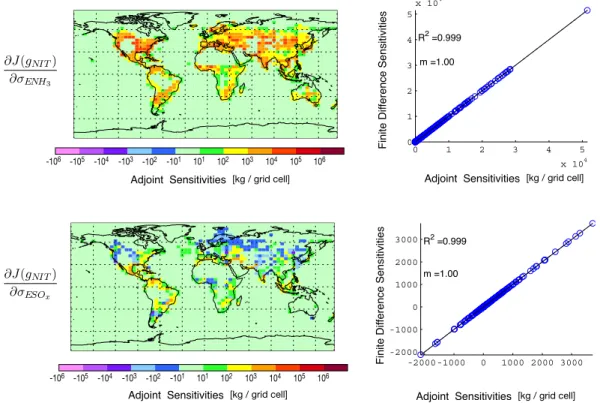
-2000 -1000 0 1000 2000 3000 -2000 -1000 0 1000 2000 3000 R2 =0.999 m =1.00 0 1 2 3 4 5 x 10⁴ 0 1 2 3 4 5 x 10⁴ R2 =0.999 m =1.00 [kg / grid cell] -106 -105 -104 -103 -102 -101 101 102 103 104 105 106 Adjoint Sensitivities F in it e D if fe re n ce Se n si ti vi ti e s F in it e D if fe re n ce Se n si ti vi ti e s [kg / grid cell] Adjoint Sensitivities [kg / grid cell] Adjoint Sensitivities [kg / grid cell] Adjoint Sensitivities -106 -105 -104 -103 -102 -101 101 102 103 104 105 106
Fig. 1. Thermodynamic adjoint validation. In the left column are the adjoint sensitivities of nitrate aerosol mass at the surface with respect to
anthropogenic NH3and SOxemissions scaling factors. In the right column are the adjoint gradients compared to finite difference gradients. The cost function is evaluated once at the end of a week-long simulation that includes only aerosol thermodynamics and emissions of SOx and NH3.
to the forward model routine to indicate which of these sub-routines to call during the adjoint calculation. Initial unequi-librated concentrations at the beginning of each external time step are saved in checkpoint files during the forward calcula-tion. Intermediate values are recalculated from these during the adjoint integration. This type of two-level checkpointing strategy has been shown to optimally balance storage, mem-ory and CPU requirements (Griewank and Walther, 2000; Sandu et al., 2005a).
The accuracy of the resulting adjoint code is tested by comparing adjoint gradients to finite difference gradients cal-culated using Eq. (17) with δσ =0.1. These comparisons can be made directly throughout the entire model domain by turning off all transport processes. Figure 1 shows compar-isons for the sensitivity of surface level nitrate aerosol mass with respect to scaling factors for emissions of surface level anthropogenic SOxand NH3after a week-long simulation.
The gradients agree quite well, confirming the accuracy of the thermodynamic adjoint code. Discussion of values of model sensitivities is given in Sect. 4.
3.2 Chemistry
KPP (v2.2) (Sandu et al., 2003; Damian et al., 2002; Daescu et al., 2003) is used to automatically generate code for the
adjoint of the tropospheric chemistry solver, which calcu-lates gradients with respect to the initial species concentra-tions. We are also interested in the gradient with respect to the emission rates for those species whose emissions are incorporated into the chemical mechanism itself, such as NOx, (as opposed to those that are simply injected into the
model grid cells at intermediate times, such as SOx). The
ad-ditional equations for calculating discrete adjoint gradients with respect to reaction rate constants are derived in Ap-pendix B. Though these equations have not been presented previously, KPP does provide the necessary subroutines for solving them.
To assess the accuracy of the adjoints of the chemistry rou-tine, we calculate the sensitivity of the species concentrations at the end of a single chemistry time step (1 h) with respect to the emissions of NOx (emitted as NO) in a box model
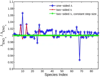
test. For this test, the chemical environment is that of a pol-luted, urban grid cell in the afternoon. Figure 2 shows the ratio λENOx/3ENOx for three separate cases. Using a
two-sided finite difference calculation (Eq. 17) with δσENOx=0.1
leads to agreement within a few percent. The dependence of the internal time step on species concentrations is a feed-back not accounted for in the adjoint algorithm; hence, also holding the internal time step fixed at 60 s results in ratios of nearly 1.000 for all species. For comparison, the ratios when
10 20 30 40 50 60 70 80 0.9 0.92 0.94 0.96 0.98 1 1.02 1.04 1.06 1.08 1.1 Species Index λ ENO x / Λ ENO x one−sided Λ two−sided Λ
two−sided Λ, constant step size
Fig. 2. Chemistry adjoint validation. The ratios of the adjoint
to finite difference sensitivities of each species with respect to NOx emissions are calculated for a 1 h box model simulation. Results are shown for a one-sided finite difference calculation, δσ = 0.1 (blue
⋄’s), a two-sided finite difference calculation (i.e. average of δσ =0.1
and −0.1, red x’s) and a two-sided finite difference calculation with a fixed internal time step of 60 s (green o’s).
Eq. (18) is used for 3ENOx are also shown, which can differ
as much as 8% from unity, demonstrating the nonlinearity of such chemical systems.
The above test was reassuring, yet limited in scope for a global CTM. To test our adjoint model over a wide vari-ety of chemical conditions, we also compare the accuracy of the adjoint derivatives of the chemical mechanism in global simulations over much longer time scales. We turn off all transport related processes in the model and calculate the ad-joint and finite difference sensitivities of surface level tracer masses with respect to NOxemissions in each location after
a week-long simulation. As lack of transport leads to unre-alistically extreme concentrations, emissions are reduced by an order of magnitude to prevent the chemical systems from becoming too stiff. Many chemical changes associated with aerosols are treated separately from the main tropospheric chemistry mechanism in GEOS-Chem, such as aqueous re-actions, dry deposition, chemical aging, and emission of SOx
and NH3(Park et al., 2004). The adjoints of these processes
are constructed separately (manually and with TAMC) and included in the following tests.
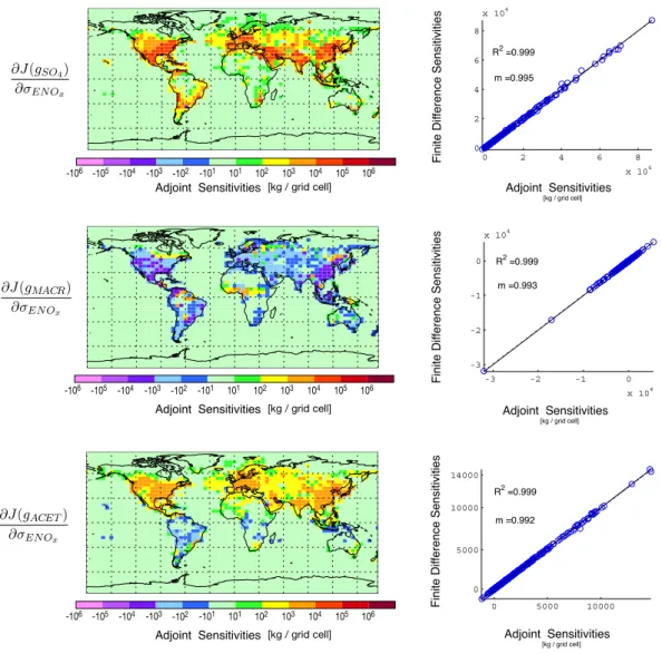
Figure 3 shows the adjoint and finite difference sensitivi-ties of several species with respect to surface level, anthro-pogenic NOxemissions scaling factors. We choose to show
sensitivities of species such as acetone and methacrolein to NOxemissions to also highlight the potential value of the
ad-joint model for analysis of non-aerosol species. We see from these, and similar tests for other active species (not shown), that the sensitivities calculated using the adjoint model con-sistently agree with those using the finite difference method over a wide range of conditions.
The code generated by KPP allows computation of either the continuous or discrete adjoints of the chemical mecha-nism. The continuous adjoint equation can be solved faster than the discrete adjoint equation at a given tolerance level, as calculation of the latter requires recalculation of inter-mediate values from the forward integration and computa-tion of the Hessian during the adjoint integracomputa-tion, see Ap-pendix B. At tight tolerance levels (i.e. very small internal time steps), the results of these methods should converge. However, for tolerance levels appropriate for global model-ing, the continuous adjoint is only approximate, as λ+δλ, where ||δλ||<C·T ol. Given that the computational expense of the Rosenbrock solver increases substantially for tighter tolerance levels (see Appendix A), it is more efficient to use the discrete adjoint, even though this requires an additional forward integration. This is in contrast to the approach of Errera and Fonteyn (2001), who chose to approximate the necessary intermediate values by linearly interpolating from values stored at each external time step, an approach likely more appropriate for their stratospheric chemistry applica-tion.
GEOS-Chem accounts for the effect of aerosol concentra-tions on the radiation available for photolysis reacconcentra-tions and on the available surface area for the heterogeneous reactions included in the main chemical mechanism. The influence of the concentration of sulfate-ammonium-nitrate aerosols on such rates is not currently accounted for in the adjoint model. We assume such an effect is less than 5% (Liao et al., 1999; Martin et al., 2003), especially as the absorbing aerosols (black carbon, mineral dust) are not active variables during these tests. The general agreement between λ and 3, only the latter of which accounts for this effect, indicates this assumption is adequate, at least for simulations of this length. Further tests indicate that this assumption is valid for most, though not all, cases, see Sect. 3.5.
3.3 Convection, turbulent mixing, and wet removal Wet removal of tracers in GEOS-Chem is generally treated as a first-order process, leading to discrete forward model equations of the form,
cn+1k = cnke−rw,k△t (19)
Since the loss rate rw,kfor most species does not depend on
any active variables (Jacob et al., 2000), the corresponding adjoint is simply
λnk = λn+1k e−rw,k△t (20)
The adjoints of these routines are generated using hand-created code, retaining efficiency and legibility. However, the in-cloud formation and cycling of sulfate aerosol from SO2 is decidedly nonlinear, as the soluble fraction of SO2
is limited by availability of H2O2, and a fraction of the SO2
is reintroduced into the gas phase as sulfate when droplets evaporate (Park et al., 2004). Such nonlinearities that span
[kg / grid cell] -106 -105 -104 -103 -102 -101 101 102 103 104 105 106 F in it e D if fe re n ce Se n si ti vi ti e s [kg / grid cell] Adjoint Sensitivities F in it e D if fe re n ce Se n si ti vi ti e s Adjoint Sensitivities [kg / grid cell] -106 -105 -104 -103 -102 -101 101 102 103 104 105 106 Adjoint Sensitivities 0 2 4 6 8 x 10⁴ 0 2 4 6 8 x 10⁴ R2 =0.999 m =0.995 -3 -2 -1 0 x 104 -3 -2 -1 0 x 104 R2 =0.999 m =0.993 0 5000 10000 0 5000 10000 14000 R2 =0.999 m =0.992 -106 -105 -104 -103 -102 -101 101 102 103 104 105 106 [kg / grid cell] Adjoint Sensitivities [kg / grid cell] Adjoint Sensitivities F in it e D if fe re n ce Se n si ti vi ti e s [kg / grid cell] Adjoint Sensitivities
Fig. 3. Chemistry adjoint validation. In the left column are the adjoint sensitivities of sulfate (SO4), methacrolein (MACR), and acetone
(ACET) at the surface with respect to surface level anthropogenic NOxemissions scaling factors. In the right column are the adjoint gradients compared to finite difference gradients. The cost function is evaluated once at the end of a week-long simulation with only chemistry and emissions × 0.1.
multiple program modules are treated both manually and with the help of TAMC, requiring additional recalculation and checkpointing of intermediate values.
Turbulent mixing in the boundary layer in the forward model is calculated according to a mass-weighted mixing algorithm applied every dynamic time step (30 min for our case), µn+1k,j = PL l=1mlµnk,l mT (21)
where µk,j is the mixing ratio (c/ρ, ρ is the density of air)
of tracer k in layer j , ml is the air mass in a single layer l, mT is the total air mass in the boundary layer column, and L
is the number of layers in the boundary layer. Rewritten in
matrix form, this equation reads,
µk,1 .. . µk,L n+1 = m1 mT · · · mL mT .. . . .. ... m1 mT · · · mL mT · µk,1 .. . µk,L n (22)
Direct application of Eq. (11) yields the corresponding ad-joint equation, λµk,1 .. . λµk,L n = m1 mT · · · m1 mT .. . . .. ... mL mT · · · mL mT · λµk,1 .. . λµk,L n+1 (23)
which can be simply written as,
λnµ k,j =
mjPLl=1λn+1µk,l mT
Deep convection is calculated in the forward model using cumulus cloud fluxes and an RAS type algorithm, see Ap-pendix A of Allen et al. (1996). We calculate the discrete ad-joint of this scheme using TAMC, noting that TAMC initially generates code that is accurate, yet several orders of magni-tude slower than necessary due to several superfluous loops that have to be removed manually. The numerical scheme for the forward calculation iteratively solves a set of essentially linear equations, with an internal time step of five minutes. If we neglect a single conditional statement that checks only for rare floating point exceptions, then storage or recalcula-tion of the intermediate values is not required for the adjoint calculation.
The adjoint model performance for a simulation including convection, turbulent mixing, and wet deposition is tested by comparison of finite difference sensitivities to the ad-joint sensitivities of concentrations of a soluble tracer with respect to its initial concentrations in a location exhibiting strong convection, deposition, and mixing. Horizontal trans-port, chemistry, and aerosol thermodynamics are turned off for these tests. We use a perturbation of one percent for the finite difference calculation. The ratio λc/3cfor simulations
that are 6 h, 1 d and 3 d in length are 0.9998, 1.0002 and 1.0003, from which we see consistent satisfactory agreement between the two methods. Performance is similar in other tested locations.
3.4 Advection
We implement the adjoint of the continuous advection equa-tions. GEOS-Chem nominally employs a monotonic piece-wise parabolic (PPM) advection routine (Colella and Wood-ward, 1984; Lin and Rood, 1996). Below we briefly show how this scheme can be used to solve the continuous adjoint advection equations and afterwards address some of the is-sues wedded to this approach. We consider the 1-D example of the advection equation for a tracer in mass concentration units,
∂c
∂t = −
∂(uc)
∂x (25)
where u is the wind velocity in the x-direction. The forward numerical model actually solves the flux form of Eq. (25) in terms of the mixing ratio (Lin and Rood, 1996),
∂(ρµ)
∂t = −
∂(ρµu)
∂x (26)
Assuming that the continuity equation for ρ is satisfied, this can be rewritten in the advection form,
∂µ
∂t = −u
∂µ
∂x (27)
Applying the adjoint variable as a Lagrange multiplier and integrating by parts (see, for example, Appendix A of Sandu et al., 2005a), the continuous adjoint of Eq. (27) is
−∂λµ
∂t =
∂(λµu)
∂x (28)
where λµ is the adjoint of the mixing ratio. Note that we
have assumed that the winds (or any other met fields) are not active variables; taking the adjoint with respect to the me-teorology is another task in itself (see, for example, Giering et al., 2005). Applying the simple transform ˆλµ=λµ/ρ, and
substituting this into Eq. (28), we arrive at the following ad-joint equation,
−∂(ρ ˆλµ)
∂t =
∂(ρ ˆλµu)
∂x (29)
which is similar in form to Eq. (26). If we assume that ρ is relatively constant over a single dynamic time step and that the advection is linear, then we can simply solve Eq. (29) us-ing the same numerical code that was used to solve Eq. (26) in the forward model, scaling the adjoint by 1/ρ before and re-scaling by ρ afterwards, which is equivalent to solving Eq. (28).
While the continuous approach was in part adopted for reasons of practicality (the discrete advection algorithm in the forward model not being directly amenable for use with automatic differentiation tools), subsequent investigation in-dicates that the continuous approach is suitable, if not prefer-able. This is not surprising, as it is well documented that discrete adjoints of sign preserving and monotonic (i.e. non-linear and discontinuous) advection schemes are not well be-haved and can contain undesirable numerical artifacts, see for example Thuburn and Haine (2001), Vuki´cevi´c et al. (2001), and Liu and Sandu (2006)2.
To illustrate the benefits of the continuous adjoint ap-proach for our system, the following numerical test is per-formed. The sensitivity of aerosol concentrations with re-spect to concentrations in a neighboring cell six hours earlier are calculated for a meridional cross section of the northern hemisphere. To afford simultaneous calculation of finite dif-ference and adjoint sensitivities throughout this domain, only horizontal advection in the E/W direction is included in these tests. Figure 4 shows finite difference sensitivities calculated using Eq. (18) for several values of δσ as well as the adjoint gradients. The undesirable nature of the finite difference sen-sitivities is indicated by negative sensen-sitivities that have no physical meaning. That negative values become more preva-lent as δσ →0 indicates such values are caused by disconti-nuities in the discrete algorithm (Thuburn and Haine, 2001). We can expect that adjoint sensitivities of the discrete advec-tion algorithm would contain similar features, which, despite being numerically precise gradients of the cost function, can result in convergence to undesirable local minimums for data assimilation (Vuki´cevi´c et al., 2001). Given the importance of transport for analysis of aerosols, use of the continuous ap-proach is deemed preferable to implementing a linear trans-port scheme with well-behaved discrete adjoints at the cost of forward model performance.
2Liu, Z. and Sandu, A.: Analysis of Discrete Adjoints of Numer-ical Methods for the Advection Equation, Int. J. Numer. Meth. Fl., submitted, 2006.
(a) Continuous adjoint sensitivities (b) Finite difference sensitivities,
(c) Finite difference sensitivities, (d) Finite difference sensitivities,
Fig. 4. Sensitivities of aerosol concentrations with respect to concentrations in adjacent cells 6 h earlier considering only E/W advection.
Sensitivities are calculated using: (a) continuous adjoint equation and (b)–(d) one-sided finite difference method with perturbations of δσ . The finite difference sensitivities contain more extreme values, including physically meaningless negative sensitivities that become more prevalent as δσ →0.
3.5 Combined performance
Again we compare the gradients calculated using the adjoint model to those calculated using the finite difference method, this time including all model processes. We calculate the sen-sitivity of global aerosol distributions of sulfate, ammonium, and nitrate to surface emissions of anthropogenic SOx, NOx
and NH3in select locations. As noted previously, such
com-parisons are quite time consuming to perform on a global scale owing to the expense of the finite difference calcula-tions. Attempting to cover a wide range of conditions, while keeping the number of required calculations within reason, we choose to analyze ten locations for each set of emissions considered, see Fig. 5. The simulations are one day in length, and the cost function (Eq. 2) is evaluated only once at the end of the day. We use a perturbation of δσ =0.1 and Eq. (18) for the finite-difference calculations.
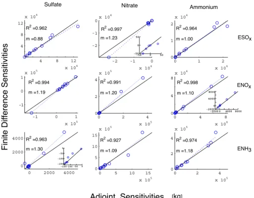
Figure 6 shows the adjoint gradients compared to the fi-nite difference gradients for each of nine relationships. From visual inspection of the scatter plots, it is clear that the agree-ment is generally within reason given the fact that using a continuous adjoint for advection is expected to cause some amount of discrepancy. Regression lines, slopes, and R2 val-ues are given for each set of comparisons. The absolute dif-ference between the two methods is often more substantial
Fig. 5. Select points for accuracy tests. Black locations used for
anthropogenic emissions of SOxand NOx, grey points for NH3, with one overlapping pair in Europe.
for the larger values. As the gradients in a given set usually span several orders of magnitude, many of the slopes are bi-ased by a few such larger values and are not representative of the overall fit. However, accounting for such heteroscedastic-ity by re-scaling the gradients by 1/p or performing weighted regressions that place less emphasis on the larger values still leads to the same general results. Picking twice as many test cells, different test cells, or a different value of δσ also was not found to substantially alter the overall comparisons.
4 8 12 x 104 4 8 12 x 104 R2 =0.962 m =0.88 -2 -1 0 x 104 -2 -1 0 x 104 R2 =0.997 m =1.23 0 1 2 x 10⁴ 0 1 2 x 10⁴ R2 =0.964 m =1.00 -1 0 1 x 10⁵ -1 0 1 x 10⁵ R2 =0.994 m =1.19 0 2 4 x 10⁵ 0 2 4 x 10⁵ R2 =0.991 m =1.20 0 4 8 x 10⁴ 0 4 8 x 10⁴ R2 =0.998 m =1.10 0 2000 4000 0 2000 4000 R2 =0.963 m =1.30 0 5 10 15 x 105 0 5 10 15 x 105 R2 =0.927 m =1.09 0 2 4 x 10⁵ 0 2 4 x 10⁵ R2 =0.974 m =1.18 -150-100 -50 0 -150 -100 -50 0 -50 0 50 -50 0 50 -2000 0 4000 8000 -2000 0 4000 8000 ESOx ENOx ENH3
Sulfate Nitrate Ammonium
F
in
it
e
D
if
fe
re
n
ce
Se
n
si
ti
vi
ti
e
s
Adjoint Sensitivities
[kg]Fig. 6. Full model performance. Comparison of sensitivities of global aerosol burdens (kg) to anthropogenic precursor emissions scaling
factors calculated using the adjoint method vs. the finite difference method. A few of the plots contain insets with magnified views of a cluster of points.
Initial comparison (not shown) of gradients for five of the 90 tests showed underestimation of adjoint sensitivities by more than an order of magnitude. Four of these tests were for the sensitivity of sulfate with respect to NH3emissions
while one was for the sensitivity of nitrate with respect to SOx emissions. Using offline concentrations for
calcula-tion of the contribucalcula-tion of sulfate aerosol to photolysis rates and heterogeneous reaction probabilities in the main tropo-spheric chemical mechanism for these tests alleviated the dis-crepancy, demonstrating that while this feedback is generally negligible, it is occasionally quite strong. Future work will extend the adjoint model to account for this feedback.
Napelenok et al. (2006) performed a complementary anal-ysis on a regional scale, calculating the sensitivities of lo-cal aerosol distributions with respect to domain-wide precur-sor emissions over the United States with a forward sensitiv-ity method (DDM-3D), using finite-difference calculations to check their results. While they found similarly good agree-ment for the more direct relationships (such as sensitivity of sulfate with respect to SO2 emissions, or ammonium with
respect to NH3emissions), they had difficulty verifying the
variability in the sensitivities of some of the more indirect relationships (such as the sensitivity of sulfate to NH3
emis-sions or nitrate to SO2 emissions). Granted, they used the
more complex and rigorous thermodynamic model ISOR-ROPIA; they suggested that such discrepancies were due to
numerical diffusion, with spatial oscillations of the sensitivi-ties indicative of errors due to transport.
In our tests, transport does not drastically degrade the con-sistency of the correlation between the two approaches; all of the R2 are near unity. There is, however, some amount of bias in the comparisons, as indicated by slopes ranging from 0.8 to 1.3, and this does appear to be a result of trans-port. Figure 7 contains scatter plots of the sensitivities of sulfate with respect to NOxemissions for several additional
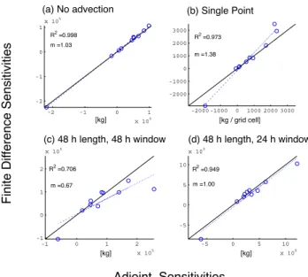
tests. Panel (a) shows the results when advection is turned off. This leads to improved agreement, m=1.03, compared to the center left panel of Fig. 6; hence, the source of this bias is presumably advection. As shown in Fig. 4, the adjoint gra-dients are likely smoother and more physically meaningful than the finite difference sensitivities.
To assess the extent to which using the continuous adjoint of advection hinders this approach to validating the adjoint model as a whole, we perform additional tests, the results of which are shown in Fig. 7. Including advection, but evalu-ating the cost function only in a single location, rather than globally, leads to a very unsmooth adjoint field and triggers many nonlinear and discontinuous aspects of the numeri-cal scheme in a manner inconsistent with advection of the relatively smooth concentration field in the forward model; hence, agreement between adjoint and finite difference gradi-ents under these conditions is worse, see panel (b). All of the
tests so far have been based on a single evaluation of the cost function at the end of a day-long simulation. The effects of changing the assimilation window (the time between consec-utive evaluations of the cost function) and the total simulation length are shown in panels (c) and (d). Doubling both the simulation length and the assimilation window to two days leads to an increased discrepancy, panel (c). Again, such be-havior is likely owing to discrepancies between the finite dif-ference and adjoint sensitivities of the advection scheme that can accumulate when integrating such sensitivities over sev-eral other nonlinear processes. Doubling only the simulation length but maintaining a one-day assimilation window im-proves the agreement, panel (d), as forcing from additional observations outweighs spurious discrepancies from advec-tion.
Finally, we consider a more realistic example. Model predictions are compared to measurements of aerosol ni-trate from the IMPROVE network of monitoring stations (http://vista.cira.colostate.edu/improve/). The sensitivities of the error weighted squared difference between predicted and observed nitrate aerosol with respect to natural NH3
emis-sions scaling factors are shown in Fig. 8. The cost function is evaluated regionally only on the U.S. East Coast (72.5◦W– 82.5◦W), and the model is run for ten days starting 1 Jan-uary 2002. Daily average measurements are assimilated dur-ing three of the ten days. Also shown is a comparison be-tween the adjoint sensitivities and finite difference sensitivi-ties evaluated for the same domain. That the overall discrep-ancy is not much different from the simple 24 h tests (Fig. 6, or Fig. 7, panel b) increases our confidence in the ability of short tests to diagnose the model’s performance in practical applications.
Overall, we find the accuracy of the adjoint gradients to be satisfactory. The adjoint model clearly captures the depen-dence of inorganic aerosol burdens on the chemical and ther-modynamic interactions that lead to their formation. While using the continuous adjoint of advection makes this veri-fication process more laborious, we have characterized the discrepancies for future reference.
3.6 Computational efficiency
Here we report computational resource requirements for run-ning the adjoint model of GEOS-Chem on a Linux worksta-tion with dual Intel Itanium 1.5 GHz processors and 4 GB of RAM. The adjoint model utilizes multiple processors on shared memory architectures as efficiently as the forward model. It requires 16 KB of checkpoint storage space per simulated day per grid cell; this amounts to 11 GB of storage space per week with the current model configuration. This is comparable to the storage requirements of other adjoint mod-els of CTMs such as STEM, 40 KB per day per cell (Sandu et al., 2005a), or the CIT model, 100 KB per day per cell (Martien et al., 2006), taking into account that the time step is 30 min in GEOS-Chem (for this study), 15 min for STEM,
-2 -1 0 1 x 10⁵ -2 -1 0 1 x 10⁵ R2 =0.998 m =1.03 -2000 -1000 0 1000 2000 3000 -2000 -1000 0 1000 2000 3000 R2 =0.973 m =1.38 F in it e D if fe re n ce Se n si ti vi ti e s
(a) No advection (b) Single Point
[kg / grid cell] [kg] -1 0 1 2 x 10⁵ -1 0 1 2 x 10⁵ R2 =0.706 m =0.67 -5 0 5 10 x 105 -5 0 5 10 x 105 R2 =0.949 m =1.00 Adjoint Sensitivities
(c) 48 h length, 48 h window (d) 48 h length, 24 h window
[kg] [kg]
Fig. 7. Effects of advection. Comparison of sensitivities of sulfate
burdens to NOxemissions scaling factors calculated using the ad-joint method vs. the finite difference method. The base case (center left panel of Fig. 6) employs the standard PPM advection scheme, and the cost function is evaluated globally once at the end of a 24 h simulation. These cases differ from the base case in the follow-ing manner: (a) advection is turned off; (b) the cost function is evaluated in only a single region; (c) both the assimilation window and total simulation length are increased to 48 h; (d) the simulation length is increased to 48 h while the cost function is evaluated every 24 h.
and 3 min for the CIT model. The computational cost of the adjoint model (backward only) of GEOS-Chem is 1.5 times that of the forward model, requiring 2.5 h for a week long iteration (forward and backward). Adjoint models of other CTMs report this ratio as: STEM: 1.5, CHIMERE: 3–4, IM-AGES: 4, Polair: 4.5–7, CIT: 11.75. We see that the adjoint of GEOS-Chem is quite efficient; in general, adjoint codes that are derived by hand or use specialized tools such as KPP are most efficient. Such efficiency is the trade-off for the la-bor involved in manually constructing an adjoint model of this size and complexity.
4 Sensitivity analysis
In this section we demonstrate how the adjoint model can be used as an efficient method of investigating the sensi-tivity of modeled aerosol concentrations to their precursor emissions. Sensitivity calculations for the full model are performed for a week-long simulation. Figure 9 shows the sensitivity of global burdens of sulfate, nitrate and ammo-nium aerosol to surface level emissions of anthropogenic SOx, NOx and NH3. The cost function is evaluated once
F in it e D if fe re n ce Se n si ti vi ti e s [unitless] Adjoint Sensitivities [unitless] Adjoint Sensitivities 0 1 2 3 0 1 2 3 R2 =0.918 m =1.25
Fig. 8. Sensitivities with respect to the error weighted squared difference between predicted and observed nitrate aerosol from the IMPROVE
network for the first ten days of January, 2002. The cost function is evaluated only on the U.S. East Coast (72.5◦W–82.5◦W). Shown are the sensitivities of the cost function with respect to natural NH3emissions scaling factors. On the right are the same quantities compared to finite difference sensitivities.
-106 -105 -104 -103-102-101 101 102 103 104 105 106
-108-107 107 108
[kg]
Sulfate Nitrate Ammonium
ESOx
ENOx
ENH3
Fig. 9. Sensitivities of global burdens of sulfate, nitrate and ammonium aerosol to anthropogenic SOx, NOxand NH3emissions scaling
factors calculated using the adjoint model for a week-long simulation.
shown) are sensitivities of these species with respect to the following emissions: stack SOx, stack NOx, biofuel SO2,
biomass burning SO2, ship SO2, biofuel NH3, biomass
burn-ing NH3, and natural NH3.
The sensitivities in Fig. 9 encompass a wide range of re-lationships between aerosols and their primary precursors. Some of these relationships are practically intuitive, such as the sensitivities of sulfate to SOxemissions or of nitrate to
NOx emissions, both of which are generally large and
pos-itive. The sensitivity of ammonium to emission of NH3 is
also positive, and the sensitivities of ammonium to SOxand
NOxemissions are always positive, owing to uptake of NH3
on inorganic aerosol by sulfate and nitrate.
Some of the relationships in Fig. 9 are less obvious, such as the negative sensitivity of sulfate to emissions of NH3.
This effect is smaller in magnitude than some of the others,
because the relationship between NH3emissions and sulfate
aerosol concentrations is less direct. As total sulfate is con-served in the MARS-A aerosol equilibrium model, this ef-fect is not due to thermodynamic interactions between am-monium and sulfate. The only species directly affected by NH3or ammonium concentrations are nitrate and nitric acid,
via thermodynamic interactions. Therefore, the relationship between NH3and sulfate is dictated by the interactions
be-tween sulfate and nitrate, and, hence, NOx. The sensitivity of
nitrate to SOx is largely negative, owing to thermodynamic
competition between nitrate and sulfate for ammonium. The sensitivity of nitrate to NH3is entirely positive, due to the
necessary presence of excess NH3 for HNO3 to condense.
The combination of these two effects explains the overall negative relationship between sulfate and emissions of NH3.
Percent Difference from Base Case -106 -105 -104 -103-102 -101 101 102 103 104 105 106 -108 -107 107 108 [kg] -90 -70 -50 -30 -10 30 < -100 10 50 70 90 > 100 [%] Percent Difference from Base Case
Fig. 10. Sensitivities of nitrate aerosol to emissions of anthropogenic NOxwhen the emission inventories are scaled by factors of 0.75 and
1.25, and the percent difference between these sensitivities and those calculated with the base case (σENOx=1.0), shown in Fig. 9.
Within the global trends noted above, there is also much discernible local variability. For example, there are a few locations where the sensitivity of sulfate to NH3emissions
changes abruptly from predominantly negative to locally positive. Some of these actually correspond to similarly abrupt shifts between areas that are sulfate-poor to areas that are sulfate-rich, such as the tip of South America and im-mediately west of the Iberian Peninsula. In other conditions or times of the day, emission of NOxcan actually lead to a
decrease in nitric acid, and, hence, nitrate.
While the adjoint model accounts for nonlinearities in the relationships between emissions and aerosols, the results of the adjoint calculation are still merely tangent linear deriva-tives (gradients) which are likely to be valid over only a lim-ited range of values for the parameters (emissions). We ex-plore the robustness of the aerosol sensitivity calculations with respect to the magnitude of the emissions. Figure 10 shows the sensitivity of nitrate with respect to NOx
emis-sions calculated when the emisemis-sions are multiplied by uni-form scaling factors of 0.75 and 1.25; the relative differences between these values and base case sensitivities shown in Fig. 9. The sensitivities can differ substantially on a point to point basis (>50%), particularly near boundaries between the positive and negative sensitivities or in areas where the sensitivities are very small. The differences are generally much less (<20%) in areas with the largest sensitivities such
as Europe, Eastern Asia and the Eastern United States. De-spite these relative differences, the sensitivity field, viewed on the global (log) scale, remains nearly identical to the base case values. While individual sensitivities may be valid only over a limited range, the sensitivity field as a whole appears fairly robust.
Overall, the adjoint model is a promising tool for examin-ing the dependence of aerosol concentrations on emissions. We note that the time required to calculate all of these sen-sitivities was less than 10 times the cost of a single forward model evaluation, while obtaining these results using the fi-nite difference method would have required >5000 times the cost of a forward run.
5 Inverse modeling tests
Several inverse modeling tests are performed to assess the ca-pabilities of the adjoint model in a data assimilation applica-tion. Using the twin experiment framework, pseudo observa-tions, cobs, are generated with the forward model using a base
set of emissions parameters, p=pa. An active subset of the
parameters used to generate these observations is then per-turbed using scaling factors, σ =p/pa, each of which is
al-lowed to vary independently in every grid cell for each emit-ted species. The inverse model uses the pseudo-observations
1 2 3 4 5 6 7 8 9 10 10−8 10−7 10−6 10−5 10−4 10−3 10−2 10−1 100 Iteration, i J i /J 1 (a) ESOx (b) ESO 2,bb (c) ESO 2,bf
Fig. 11. Cost function reduction for tests DA1. A uniform
per-turbation is applied to emission inventories of (a) SOx(b) biomass burning SO2(c) biofuel SO2. Complete daily measurements of sul-fate aerosol are utilized for the data assimilation during a week-long simulation.
to recover the original unperturbed values of these active pa-rameters.
We begin by generating a week-long set of observational data using the forward model with all scaling factors set equal to unity. For these initial tests, we perturb one set of emissions by re-scaling the emissions in every cell by a fac-tor of two, and we use observations in every grid cell once every 24 h to force the data assimilation. As there is no error in these observations, equal weight is ascribed to each (S−1obs is the identity matrix), and the error covariance of our initial (perturbed) estimate of the emissions scaling factors is infi-nite (S−1p is zero). Such conditions are unrealistic and serve only to test the adjoint model under the most ideal conditions possible.
In the first set of tests (DA1), we perturb the emission in-ventories of (a) surface level anthropogenic SOx, (b) biomass
burning SO2 and (c) biofuel SO2. We assimilate
observa-tions of sulfate for the week of 1–7 July 2001. Figure 11 shows the progression of the normalized (divided by the ini-tial value) cost function at iteration i during the optimiza-tion procedure, Ji/J1. The cost function quickly reduces by
at least five orders of magnitude in each case. The correct emissions inventories are essentially entirely recovered.
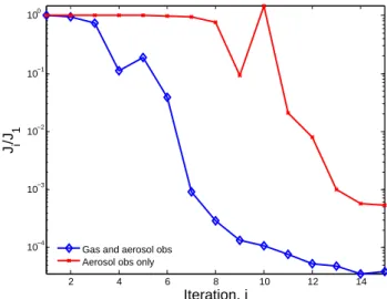
In the next test (DA2), we perturb the emission inventory of NH3 from anthropogenic sources, and assimilate
obser-vations of aerosol ammonium. This is a slightly more diffi-cult inversion as ammonium measurements alone do not fully constrain NH3emissions (Gilliland et al., 2006). As
demon-strated in Sect. 3.5, ammonium is indirectly, yet apprecia-bly, coupled to gas-phase oxidants. Utilizing observations of Ox (O3, NO2and NO3) in conjunction with ammonium
observations noticeably increases the convergence rate over
2 4 6 8 10 12 14 10−4 10−3 10−2 10−1 100 Iteration, i J i /J 1
Gas and aerosol obs Aerosol obs only
Fig. 12. Cost function reduction for tests DA2. A uniform
per-turbation is applied to emission inventories of anthropogenic NH3. Complete daily measurements of (red-crosses) ammonium aerosol and (blue-diamonds) ammonium aerosol and gas-phase Oxare uti-lized for the data assimilation during a week-long simulation.
using either type of observations alone, see Fig. 12. This demonstrates, albeit in a highly idealized fashion, the poten-tial for exploiting multi-phase measurements as constraints for aerosol modeling.
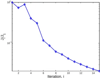
The final test (DA3) attempts to mimic a slightly more re-alistic scenario than the previous tests: improving estimates of global anthropogenic SOxand NOxemission inventories
using surface measurements of sulfate, nitrate, and ammo-nium aerosol. In this case, the emissions inventories are per-turbed regionally by 5–30% with an additional random fac-tor of order 5%. For example, the anthropogenic SOx and
NOxemissions in North America are perturbed by factors of
0.8+r and 0.85+r, respectively, while emissions in Asia are perturbed by factors of 1.2+r and 1.3+r, where r is a ran-dom number uniformly distributed between 0 and 0.05. The error covariance matrix Spis calculated using an ascribed
er-ror of 100% and is assumed to be diagonal. Observations are used once per day in only half of the land-based surface grid cells. The reduction of the cost function after 15 iter-ations is shown in Fig. 13. The difference between the true emission inventories for SOxand NOxand the estimated
in-ventory at the first and final iterations are shown in Fig. 14. While there are substantial improvements in the SOx
emis-sions and the NOxemissions in Europe and Asia, the NOx
emissions in North America have yet to converge. Although the cost function has reduced by nearly two orders of mag-nitude, the optimization procedure has clearly yet to reach a minimum. In applications of this type, the procedure is often halted according to an appropriate convergence criteria. Fur-ther iterations might be justified; however, care must be taken to avoid overly minimizing the predictive error component of the cost function at the sake of generating noisy solutions.
6 Summary and conclusions
The derivation of the adjoint model of GEOS-Chem has been presented in a piecewise fashion. We have implemented the first adjoint of an aerosol equilibrium thermodynamic model (MARS-A, Binkowski and Roselle, 2003), derived using the automatic differentiation tool TAMC (Giering and Kamin-ski, 1998), which required significant manual pre- and post-processing owing to the structure and complexity of the code. To facilitate construction of the adjoint of the GEOS-Chem gas-phase chemical mechanism, we implemented a Rosen-brock solver using the KPP numerical library (Sandu et al., 2003). This has allowed for automatic generation of the ad-joint of the chemical mechanism and also improved forward model performance (see Appendix A). The adjoints of wet removal, deep convection, and turbulent mixing were derived manually and with the aid of TAMC. We have used the con-tinuous adjoint method to treat advection, wherein the same numerical algorithm is used to solve the continuous adjoint advection equation as was used for tracer advection in the forward model.
All aspects of the adjoint model have been tested both separately and together by comparing the adjoint gradients to finite difference gradients. Each individual discrete ad-joint routine showed satisfactory performance over a wide range of conditions. The adjoint gradients of the cost func-tion evaluated using the full model are well correlated with the numerical gradients, as measured using finite difference calculations, with most R2>0.95. The hybrid approach adopted here avoids physically unrealistic noise associated with discrete adjoints of nonlinear and discontinuous advec-tion schemes and does not entirely preclude validaadvec-tion of the adjoint model as a whole via comparison to finite difference gradients. Such comparisons are understandably unrevealing when considering sparse or infrequent data; however, in both ideal test calculations with smooth adjoint forcings and real-istic tests of week-long sensitivities of predictions of actual aerosol observations, the comparisons are consistent enough to ensure proper derivation of the adjoint. Nevertheless, this treatment necessitated additional inspection of model perfor-mance on a component-wise basis. While these benchmarks set the standard for further use and development of this ad-joint model, future applications may require additional test-ing.
The adjoint model clearly demonstrates the importance and relative strengths of many complex nonlinear relation-ships connecting concentrations of aerosol species and their precursor emissions. Though indirect, relationships such as the dependence of sulfate aerosol concentrations on emission of NH3or NOxare captured by the adjoint model and can
be determined globally in an efficient manner. The sign and magnitude of many of these sensitivities exhibit a rich array of features owing to the influence of environmental factors, such as the sulfate to ammonium ratio, cloud processing of SO2, and variability in the NOxand Oxlevels.
2 4 6 8 10 12 14 10−1 100 Iteration, i J i /J 1
Fig. 13. Cost function reduction for tests DA3. Emissions
inven-tories of anthropogenic SOxand NOxemissions are perturbed re-gionally and optimized simultaneously utilizing sparse daily mea-surements of aerosol sulfate, ammonium, and nitrate during a week-long simulation.
We have also demonstrated the capabilities of the adjoint model in mock data assimilation applications. An adjoint model of this type allows for the possibility of exploiting multi-phase observations to constrain emissions of aerosol precursors. Here we have focused on regional variability of the emissions inventories, though the emissions can also be adjusted on a temporal basis. For real data assimilation projects, many application specific issues inherent in this type of inverse modeling have yet to be resolved, such as specification of the error covariance matrices Sobs and Sp.
The dependance of adjoint model performance is known to depend strongly on such factors (Chai et al., 2006), proper formulation of which is necessary to ensure scaling of the in-ventories that are physically realistic (Stavrakou and Muller, 2006). Real world application will also likely require con-ditioning of the cost function to improve convergence rate (Meirink et al., 2006) and tuning of the regularization pa-rameter (Hakami et al., 2005).
Subsequent studies will focus on expanding the adjoint model to capture feedbacks such as the effect of sulfate aerosol concentrations on photolysis rates and heterogeneous reaction probabilities, seen here to occasionally be quite im-portant. Work on the adjoint of the aerosol equilibrium model ISORROPIA (Nenes et al., 1998) is also in progress. Further application of the GEOS-Chem model will focus also on the exploitation of multi-phase measurements from sources such as surface stations, aircraft, and satellites as model constraints. The adjoint of GEOS-Chem has already been used to constrain emissions of carbon monoxide from Asia using satellite (MOPITT) measurements (Kopacz et al., 20071), demonstrating the potential for addressing a wide range of scientific questions with this type of inverse model.
-1.7x10¹¹ -4.3x10¹⁰ 7.8x10¹⁰ 2.0x10¹¹
-2.3x10³ -5.7x10³ 1.2x10⁴ 2.9x10⁴
ESOx(i=1) - ESOx(true) ESOx(i=15) - ESOx(true)
ENOx(i=1) - ENOx(true) ENOx(i=15) - ENOx(true)
[molecule / (cm2 s)]
[kg / (grid cell hour)]
Fig. 14. Emissions inventory estimates for test DA3. Difference between the estimated emission inventory at iteration i and the “true”
inventory, which was used to generate the pseudo-observations. Results are shown for the initial estimate (left column) and after 15 iterations (right column).
Appendix A
Implementation of a Rosenbrock solver and comparison to SMVGEARII
Solving large systems of chemical rate equations in CTMs requires the use of special numerical tools, or solvers, that are specifically designed for this purpose. Taking the adjoint of such solvers manually, or using generic automatic differenti-ation tools, can be an onerous task. We desire to create the adjoint of the full chemical mechanism in GEOS-Chem using the KPP software library (Sandu et al., 2003; Daescu et al., 2003; Damian et al., 2002), which is a set of tools specifically built for automatic differentiation of chemical mechanisms and the numerical algorithms used to solve these systems. In order to make use of these tools, we must first implement the KPP generated numerical integration routines in the forward model. We investigate the feasibility and ramifications of replacing the current solver in GEOS-Chem, SMVGEARII (Jacobson, 1995), with a KPP generated Rosenbrock solver. We consider the amount of work required to make such a
switch, the efficiency of the Rosenbrock solver compared to the SMVGEARII solver, and the overall effect that such a switch has on the model predictions after a week-long simu-lation.
After manually translating the SMVGEARII mechanism input files to KPP input files, the KPP tools easily generate a set of Fortran code that solves the given system for a variety of supported Rosenbrock type integrators in a box model set-ting. Minimal manual adjustment to this code was required to interface with the 3-D GEOS-Chem model and to allow support for OpenMP parallelization. Some amount of mod-ifications to the KPP code itself will be required to fully au-tomate this process.
Next we consider the efficiency of the Rosenbrock solver and the SMVGEARII solver in a global simula-tion with only chemistry. For each species, in every cell, we compare the concentrations from benchmark so-lutions at the end of a day-long simulation to concen-trations from a reference solution for each solver. The benchmark calculations span a set of tolerance levels
molecules cm−3} while the reference solutions were
com-puted using tight tolerances (RTOL=10−8, ATOL=102 molecules cm−3). RTOL and ATOL are the relative and ab-solute error tolerance levels, respectively. Looser tolerance levels result in repeated failure to converge in numerous grid cells.
To assess the accuracy of the two methods, following Sandu et al. (1997) we define the significant digits of accu-racy (SDA) as
SDA = − log10(maxkERk)
where ERk is a spatially modified root mean square norm
of the relative error of the benchmark solution ( ˆck,j) with
respect to a reference solution (ck,j) for species k in grid cell j , ERk= v u u t 1 |θk| ·X j ∈θk ck,j − ˆck,j ck,j 2
For 2 total grid cells, θk is the set of all locations of
sig-nificant concentrations of species k, {0≤θ ≤2 : ck,j≥a}. A
threshold value of a=106molecules cm−3is chosen to avoid inclusion of errors from locations where concentrations of a given species are less than chemically meaningful values.
We present the results in the form of a work – precision diagram, wherein the value of SDA for each test is plotted versus the average computational expense for the solver to integrate the chemical mechanism for one hour. When cal-culating this average, we do not consider the time required during the initial six hours of the simulation, as each solver requires a bit of “spin up” time in order to adjust internal time steps to values more appropriate than the default starting step size according to the stiffness of the local system. Such spin up time is negligible with respect to the total computational cost of any simulation longer than a few days.
Figure A1 shows the work-precision diagram for the global benchmark simulations. The Rosenbrock solver is nearly twice as efficient as the SMVGEARII solver during these tests. Based on this analysis, we choose to run the Rosenbrock solver at tolerance levels that yield an SDA of
∼1.0 as the standard setting for this work.
For practical applications, we are interested in the dif-ference in the total model predictions, including all model processes, incurred by switching to the Rosenbrock solver. We compare the daily average concentrations after a week-long simulation, including all model processes, calculated using the new standard Rosenbrock settings versus the stan-dard SMVGEARII settings. Figure A2 shows the values of ERk for each species k using the Rosenbrock solver
to generate the test solution and SMVGEARII for the reference solution. This figure shows that after switch-ing to this Rosenbrock solver, the solution is changed by less than 10% for most species. The difference is larger, between 10 and 15%, for HNO2, HNO4, IAP,
100 101 102 0 0.5 1 1.5 2 2.5 3 3.5 4 4.5 5 Time, s SDA Rosenbrock SMVGEARII
Fig. A1. Work-precision diagram for the Rosenbrock (blue circles),
and SMVGEARII (red crosses) chemical solvers. Each solver is im-plemented in the 3-D model and run for one day using a 1 h external chemical time step. Plot shows the average time taken per external chemical time step versus the significant digits of accuracy (SDA) achieved. Tests performed using dual 1.5 GHz Itanium processors.
INO2, ISOP, N2O5, NO, NO2, PP, and RIP (for full
definition of species, see http://www.env.leeds.ac.uk/∼mat/
GEOS-CHEM/GEOS-CHEM Chemistry.htm). Determin-ing whether or not this is an actual improvement in the accu-racy of the forward model itself would require further com-parison to observations. At the very least, the switch results in an improvement in the numerical solution of the forward model equations for slightly less computational cost.
Overall, while a more detailed analysis (requiring opti-mization of specific species tolerance levels and the parame-ters that control internal step size expansion and contraction) is necessary to determine unequivocally which method is more efficient, in our experience, not only is the Rosenbrock method desirable because of its differentiability, but it also appears to improve forward model performance by provid-ing more accurate solutions to the model’s chemical mech-anism than the SMVGEARII solver for less computational expense. We have reported only the results using the Rodas-3 set of Rosenbrock coefficients; however, additional tests were performed using the other available sets (Ros-2,Ros-3,Ros-4,Rodas-4), and the trends were similar. It must also be emphasized that these comparisons should not be gener-alized to other platforms or CTMs; the SMVGEARII algo-rithm is designed to perform most efficiently on vector plat-forms by re-ordering the grid cells every external chemistry time step, an operation which serves only to increase the cost of this method by ∼5% on non-vector machines such as those used in this study, and most other GEOS-Chem studies.