A mushy Earth's mantle for more than 500 Myr after the magma ocean solidification

(1)

HAL Id: hal-03059716

https://hal.archives-ouvertes.fr/hal-03059716

Submitted on 13 Dec 2020

HAL is a multi-disciplinary open access

archive for the deposit and dissemination of

sci-entific research documents, whether they are

pub-lished or not. The documents may come from

teaching and research institutions in France or

abroad, or from public or private research centers.

L’archive ouverte pluridisciplinaire HAL, est

destinée au dépôt et à la diffusion de documents

scientifiques de niveau recherche, publiés ou non,

émanant des établissements d’enseignement et de

recherche français ou étrangers, des laboratoires

publics ou privés.

the magma ocean solidification

Julien Monteux, D Andrault, M Guitreau, Henri Samuel, S Demouchy

To cite this version:

Julien Monteux, D Andrault, M Guitreau, Henri Samuel, S Demouchy. A mushy Earth’s mantle for

more than 500 Myr after the magma ocean solidification. Geophysical Journal International, Oxford

University Press (OUP), 2020, 221 (2), pp.1165-1181. �10.1093/gji/ggaa064�. �hal-03059716�

(2)

GJI Geodynamics and tectonics

A mushy Earth’s mantle for more than 500 Myr after the magma

ocean solidification

J. Monteux,

1

_{D. Andrault,}

1

_{M. Guitreau,}

1

_{H. Samuel}

2

_{and S. Demouchy}

1,3

1_{Université Clermont Auvergne, CNRS, IRD, OPGC, Laboratoire Magmas et Volcans, F-63000 Clermont-Ferrand, France. E-mail:}_{julien.monteux@uca.fr} 2_{Institut de Physique du Globe de Paris, Université Sorbonne Paris Cité, 75005 Paris, France}

3_{G´eosciences Montpellier – Universit´e Montpellier & CNRS, F-34095 Montpellier, France}

Accepted 2020 January 24. Received 2020 January 22; in original form 2019 July 17

S U M M A R Y

In its early evolution, the Earth mantle likely experienced several episodes of complete melting enhanced by giant impact heating, short-lived radionuclides heating and viscous dissipation during the metal/silicate separation. After a first stage of rapid and significant crystallization (Magma Ocean stage), the mantle cooling is slowed down due to the rheological transition, which occurs at a critical melt fraction of 40–50%. This transition first occurs in the lowermost mantle, before the mushy zone migrates toward the Earth’s surface with further mantle cooling. Thick thermal boundary layers form above and below this reservoir. We have developed numerical models to monitor the thermal evolution of a cooling and crystallizing deep mushy mantle. For this purpose, we use a 1-D approach in spherical geometry accounting for turbulent convective heat transfer and integrating recent and solid experimental constraints from mineral physics. Our results show that the last stages of the mushy mantle solidification occur in two separate mantle layers. The lifetime and depth of each layer are strongly dependent on the considered viscosity model and in particular on the viscosity contrast between the solid upper and lower mantle. In any case, the full solidification should occur at the Hadean–Eoarchean boundary 500–800 Myr after Earth’s formation. The persistence of molten reservoirs during the Hadean may favor the absence of early reliefs at that time and maintain isolation of the early crust from the underlying mantle dynamics.

Key words: Numerical modelling; Heat flow; Rheology: Mantle; Dynamics: convection currents, and mantle plumes; Heat generation and transport.

1 . I N T RO D U C T I O N

After the giant impact which led to the formation of the Earth– Moon system, the Earth’s mantle was likely completely molten (e.g. Nakajima & Stevenson2015). During the subsequent Magma Ocean (MO) stage, the Earth’s early mantle undergone a rapid global cooling until its melt fraction decrease to a critical value ϕc

(≈40%) associated with a major increase of its viscosity (Solomatov 2007; Monteux et al. 2016). This step was followed by a slow cooling stage that triggered a complete crystallization of the silicate mantle (Solomatov2007). This second cooling stage could have lasted hundreds of Ma, or even a couple of Ga as its dynamics was governed by the rheology of the slowly deforming solid-like mantle, in contrast to the first one which was driven by the magma viscosity (Solomatov2007; Ulvrov´a et al.2012; Monteux et al.2016).

Recent experimental results have shown that the upper man-tle solidus is at lower temperature than previously expected for a chondritic composition (Andrault et al.2018). According to this study, such a solidus associated with a hotter earlier mantle would enable the presence of a deep and persistent molten layer in the

Archean mantle. The progressive solidification of this melt layer could have enhanced the mechanical coupling between the litho-sphere and the asthenolitho-sphere. Such a change might explain the transition from surface dynamics dominated by a stagnant lid to modern plate tectonics with deep-slab subductions. Assuming that the intersect between the mantle solidus and an adiabat tempera-ture profile with a potential surface temperatempera-ture corresponding to a surface melt fraction of ϕc≈ 40% could constrain the depth of the

bottom of the remaining partially molten layer, Solomatov (2007) obtained a depth ≈300 km. In the case of bottom-up solidification of a mushy mantle, the depth of the last remaining partially molten layer should, hence, be smaller than 300 km and the full mantle crystallization should occur within ≈1 Ga (Sleep et al.2014).

The depth at which the full crystallization is reached is likely gov-erned by (1) the solidus temperature which controls the depth and temperature of solidification, (2) the thickness of the top thermal boundary layer (TBL), where heat convecting from the deep mantle is transferred to the surface by conduction and (3) the temperature contrast on both sides of the TBL which controls the efficiency of heat evacuation. In the mushy regime, the mantle viscosity is a

C

⃝The Author(s) 2020. Published by Oxford University Press on behalf of The Royal Astronomical Society. 1165

Downloaded from ht tps: //academic. oup. com/ gji/ art icle-abst ract /221/ 2/ 1165/ 5721374 by INF U B IB LI O P LA NE T S user on 04 May 2020

(3)

key parameter, which governs mantle dynamics and the formation of TBLs. This day viscosity of the Earth’s mantle is difficult to constrain, particularly in the lower mantle ( ˇC´ıˇzkov´a et al.2012), and the value of the viscosity of the Earth’s early mantle prior to the occurrence of major differentiation events is even more hypo-thetical. Constraining the value of this physical quantity is of first importance, since deep mantle viscosity likely governs the initia-tion of major geological features, such as plate tectonics and mantle plumes (Sleep2014; Foley et al.2014).

We have developed a numerical model to monitor the cooling, and crystallization of an isochemical mantle, starting from a partially molten stage. We aim to characterize the influence of the viscosity of the solid early mantle on its cooling dynamics. In particular, we tested the impact of variation in activation energy and the viscosity prefactor, as well as monitored the cooling and crystallization pro-cesses to determine the solidification timescales and the depths at which the last melt fraction solidifies.

2 . M O D E L

We considered the cooling of a partially molten magma ocean with an initial depth of 2900 km, which we modelled using a thermal evolution described below.

2.1 Thermal evolution model 2.1.1 Heat transfer model

We used a 1-D spherical approach (e.g. Abe1997; Laneuville et al.

2018) accounting for turbulent convective heat transfer (e.g. Abe 1997; Monteux et al.2016; Bower et al.2018). This approach is relevant for the ranges of low viscosities and high Rayleigh num-bers expected within a partially molten planetary mantle which are difficult to numerically resolve in 2-D and 3-D spatial domains. Indeed, even if Ra numbers are lower during the mushy stage than during the magma ocean stage, Ra numbers are still too high (up to 1030_{) to correctly solve the TBLs in such a dynamic reservoir.}

Moreover, molten reservoirs may survive during the early thermal evolution of the mushy mantle. In these regions, the melt fraction can reach values larger than 40% with very low associated viscosity of the mushy material, making the local Rayleigh number too high for 2-D or 3-D computational domains.

Our numerical model solves the following heat equation: ρCp

∂T

∂t = ∇. (k∇T ) + ρ H, (1) where ρ is the density, Cp is the heat capacity, T is the

tempera-ture and H is the heat production from radiogenic sources. k is an ‘effective’ conductivity defined as:

k = kc + kv, (2)

with kvthe effective conductivity relative to thermal convection of

the mushy material is:

kv =

FconvL

$T , (3)

Fconvis the convective heat flux accounting for thermal buoyancy,

L is the thickness of the Earth’s mantle and kcthe intrinsic thermal

conductivity of the material (kc= 5 W.m−1.K−1).

For mantle convection to occur, the temperature gradient must be larger than the adiabatic gradient:

!_dT dr " S = −αgT Cp . (4)

When the temperature gradient is subadiabatic, the mantle heat is transported only by conduction, and k = kc. When the temperature

gradient is superadiabatic, the mantle is convecting. The convective heat flux Fconvdepends on the local Rayleigh number Ra:

Ra =αgCpρ_k2$T L3

cη , (5)

where α is the thermal expansion coefficient of the mushy material,

g is the gravitational acceleration assumed to be constant through

the whole mantle and η is the local dynamic viscosity. In eq. (5),

kcis constant, Cp is a function of the melt fraction, α and ρ vary

with depth and melt fraction. η varies with depth, temperature and melt fraction. $T is the thermal driving force for the convection, therefore the temperature difference between the surface and the core–mantle boundary (CMB) minored by the increase of tempera-ture along the mantle adiabat. Mantle dynamics and cooling is also governed by the Prandtl number, Pr:

Pr = η_kCp c

, (6)

which is the ratio of the momentum diffusivity over the thermal diffusivity. Pr is calculated at each depth using the local viscosity value η. Depending on the values of Pr and Ra, two flow regimes arise and as a consequence two convective heat fluxes:

(1) a soft turbulent regime where the corresponding convective heat flux is (Solomatov2007; Monteux et al.2016):

Fconv=

0.089kc$T Ra1/3

L if Ra < 10

8_Pr5/3_; _(7a)

(2) and a hard turbulent regime (following Solomatov 2007; Monteux et al.2016) where:

Fconv= 0.22kc

$T Ra2/7_Pr−1/7

L if Ra > 10

8_Pr5/3_. _(7b)

In our numerical model, we compare the temperature gradient to the adiabatic gradient. If the temperature gradient is larger, kvis

calculated according to eq. (3). If the temperature gradient is lower,

k = kc.

2.1.2 Boundary and initial conditions

The large impacts, radiogenic heating and the energy dissipated during metal-silicate separation control the early thermal state of the core. The core temperature at the end of the magma ocean stage is governed by the heat accumulated in this reservoir during its formation but also by the efficiency of the magma ocean to retain heat within the core by forming thick TBLs (Monteux et al.2016). The core heat flow at the CMB can be expressed as:

Fcore=

kc#Tcore− TCMBmantle

$ δTBL,bot

, (8)

where Tcore _{is the average core temperature just below the CMB}

(i.e. here, a TBL within the core is not considered) and Tmantle CMB is the

mantle temperature above the CMB. δTBL,botis the thickness of the

TBL at the bottom of the mantle where the heat is extracted from the core by conduction. Tmantle

CMB is calculated form eq. (1) whereas Tcore

(4)

is obtained by the integration of the following differential equation:

VcoreρFeCp,Fe

dTcore

dt = ScoreFcore, (9) where Vcoreis the core volume, Scoreis the core surface, ρFeis the

core density, Cp,Feis the core heat capacity. This formulation does

not consider the increase in adiabatic temperature within the core but allows following the evolution of core temperature right below the CMB as a function of time, based on the CMB heat flux. The error associated with this simplification (which in the case of an Earth-like body would amount to less than 10%) is small compared to uncertainties in other model parameters.

The efficiency of mantle cooling also depends on the heat transfer at the surface. During the magma ocean cooling, heat is efficiently radiated toward space, but the formation of a primitive atmosphere may significantly slow down the cooling. With a primitive atmo-sphere composed of 300 bars H2O and 100 bars CO2 overlaying

the magma ocean, Lebrun et al. (2013) estimated that the surface temperature remains constant throughout the entire duration of the mushy stage at Tsurf≈ 500 K. Sleep et al. (2014) also showed that

the surface temperature during the mushy stage was maintained at ≈500 K for 1000 bars and 100 bars atmospheres in equilibrium with bulk silicated magmas.

2.1.3 TBLs parametrization

Monteux et al. (2016) showed that the initial core heat can only be efficiently retained within the core when the bottom TBL thickness (δTBL,bot) is larger than ≈100 m. For δTBL,bot<100 m the thermal

cou-pling between the core and the MO is important and the core’s heat is efficiently transferred to the mantle during the short timescales of the MO cooling. For δTBL,bot<1 m, the core rapidly cools down

to ≈4400 K, which corresponds to the core-mantle boundary tem-perature at a critical melt fraction ϕ = ϕcrit. Actually, the thicknesses

of both the bottom and top TBL are governed by the cooling dy-namics of the mantle (Solomatov1995). The formation of a TBL is induced by the velocity field decrease close to the boundary. In 1-D models, the TBL cannot form numerically by themselves be-cause the velocity field is not calculated and, hence, it has to be parametrized. Moreover, as we consider a compressible fluid with properties changing with depth, the top and bottom TBL do not have the same thicknesses. In our models, we consider that the thermal boundary thickness scale as (Grott & Breuer2008):

δTBL= L !_Ra crit Ra "1/3 , (10)

with Racrit= 450 (Choblet & Sotin2000) and Ra is the Rayleigh

number value calculated using eq. (5) and the characteristic param-eters corresponding to either the top or the bottom of the magma ocean, for upper and lower TBL, respectively. It results in a TBL thicker at the top of the mantle, than at the bottom of the mantle. Strictly, the value of Racritshould be different when considering

the upper or lower TBL (Thiriet et al.2019). The value of 450 is adapted for the upper mantle. For the lower mantle, it should be ex-pressed as a function of the internal Rayleigh number (Deschamps & Sotin2000). We have implemented such a parametrization in our models. Our numerical tests (not shown here) show that the bottom TBL thickness derived from Deschamps & Sotin (2000) leads to a decrease of the bottom TBL thickness, but does not change sig-nificantly the solidification depth and time scales. Hence, we used

Racrit= 450 for both top and bottom TBL calculations. Within the

TBLs, the heat is transferred by conduction and, again, k = kc. In

all the models presented here, the TBL thickness has a thickness larger than 10 km, therefore given our 1-km grid spacing, at least 10 gridpoints are used to identify and characterize the heat transfer in the TBL.

2.2 Geochemical model and derived parameters

Despite the difficulty to characterize the chemical composition of the Earth’s early mantle, a consensus has emerged that Earth’s man-tle should be of chondritic composition (e.g. Mc Donough & Sun 1995; Javoy et al.2010; Palme & O’Neill2014). Still, chondrites present a large diversity in major, minor and trace element composi-tions. According to several isotopic tracers, Earth has accreted from a large majority of building blocks typical of high-enstatite chon-drites (EH, Javoy et al.2010). Then, late-accretion processes and core–mantle differentiation (Rubie et al.2011) have induced a drift of the bulk mantle composition to an MgO-enriched composition, compared to EH (e.g. Mc Donough & Sun1995; Palme & O’Neill 2014). In the following section, we detail our chemical model for the mushy mantle following the magma ocean stage.

2.2.1 Radiogenic heating

Short timescales inferred for the duration of the magma ocean stage appear comparable to the timescales for the decay of short-lived radionuclides such as26_{Al. However, large bodies such as the}

proto-Earth, or the Theia Earth’s impactor, appeared only much later, from the accretion of pre-differentiated planetesimals. Therefore, only the long-lived radiogenic elements, such as238_U,235_U,232_Th

and40_{K can provide heat at the long time scale corresponding to}

the cooling of the mushy mantle. In our models, we consider the radiogenic heating from these radionuclides in eq. (1) assuming that the abundance of these elements in the primitive mantle is similar to the concentration in EH-chondrites (Javoy1999). The radiogenic heat production rate is computed as:

H = ( Ai[i] Hiexp (−λi(t − t0)) , (11)

where the meaning of Ai, Ei, Hi, λiis detailed in Table1.

2.2.2 Solidus and liquidus temperatures

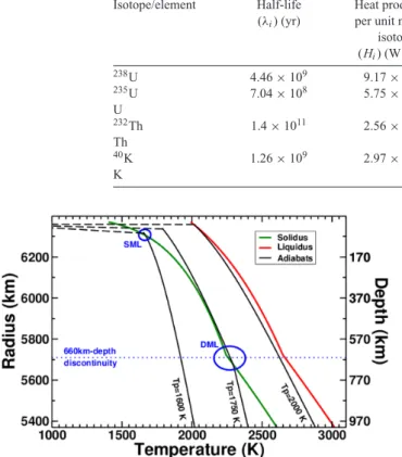
The chemical composition of the mantle governs its melting proper-ties, based on its solidus and liquidus profiles. The latter plays a ma-jor role in the early thermal evolution of the magma ocean, because it defines the temperature and the depth at which crystallization starts. Laboratory experiments have constrained the liquidus and solidus of mantle-like material up to pressures compatible with the CMB conditions (Fiquet et al.2010; Andrault et al.2011). We performed calculations using the melting curves derived from chondritic-type mantle composition from Andrault et al. (2011,Fig.1). The experi-mental solidus and liquidus profiles are fitted with a modified Simon and Glatzel equation (Simon & Glatzel1929). For pressures P be-low 24 GPa, we use solidus and liquidus temperatures of chondritic mantle reported from Andrault et al. (2018):

Tsol= 1373. ! _P 0.82 × 109 + 1 "(1/6.94) , (12a) Tliq= 1983.4 ! _P 6.48 × 109 + 1 "(1/5.35) . (12b) Downloaded from ht tps: //academic. oup. com/ gji/ art icle-abst ract /221/ 2/ 1165/ 5721374 by INF U B IB LI O P LA NE T S user on 04 May 2020

(5)

Table 1. Radiogenic heat sources and characteristics (from Javoy1999).

Isotope/element Half-life Heat production Natural Present-day

(λi) (yr) per unit mass of Abundance concentrations

isotope (Ai) (%) ([i]) (ppm wt.) (Hi) (W kg−1) 238_U _{4.46 × 10}9 _{9.17 × 10}−5 _99.28 235_U _{7.04 × 10}8 _{5.75 × 10}−4 _0.72 U 0.20 232_Th _{1.4 × 10}11 _{2.56 × 10}−5 ₁₀₀ Th 0.069 40_K _{1.26 × 10}9 _{2.97 × 10}−5 _0.0117 K 270

Figure 1. Solidus (green) and liquidus (red) (computed from eq. 12) as a function of the Earth’s radius. Black solid lines show adiabatic temperature profiles (computed from eqs4and18) with three different potential temper-atures (1600, 1750 and 2000 K). Note that these three temperature profiles are arbitrary and do not result from our numerical model. The blue dashed line separates the upper and lower mantle. The dashed lines correspond to the hypothetic conductive temperature profiles in the top thermal boundary layer (i.e. recalculated at each step of our modelling procedure). The two ellipsoids illustrate critical points where deep and shallow last molten layers should solidify (SML, shallow mantle layer and DML, deep mantle layer).

For pressures larger than P = 24 GPa, we use results from An-drault et al. (2011): Tsol= 1334.5 ! _P 9.63 × 109 + 1 "(1/2.41) , (12c) Tliq= 1862. ! _P 21.15 × 109 + 1 "(1/2.15) . (12d) Mantle solidification may induce some chemical fractionation. In such case, the melting curves may evolve (Andrault et al.2017). Major changes concern the liquidus temperature, which increases with the MgSiO3-content in the mantle. On the other hand, the

man-tle’s solidus is almost independent of composition. These effects are not accounted in our study, because there is an insufficient knowl-edge on melting properties as a function of pressure, temperature and mantle composition.

2.2.3 Thermodynamic parameters

Thermodynamic parameters of the magma ocean depend of its chemical composition. Volumetric and elastic parameters of silicate liquids have been characterized up to a pressure of 140 GPa using shock compression experiments (Mosenfelder et al.2007,2009;

Thomas et al.2012; Thomas & Asimow2013). Here we assume a multicomponent system with a chondritic-type composition (62% enstatite + 24% forsterite + 8% fayalite + 4% anorthite + 2% diop-side). Using fourth-order Birch-Murnaghan/Mie-Gr¨uneisen equa-tion of state fits for molten silicate liquids from Thomas & Asimow (2013), we obtain the melt density ρm, the volumetric thermal

ex-pansion α as a function of pressure as well as the specific heat Cpof

the molten material for a chondritic multicomponent assemblage. The density of the solid phase is then calculated as:

ρs = ρm + $ρ, (13)

with $ρ being the density difference between solid and liquid phases which is fixed to 64 kg m−3_{(Monteux et al.}₂₀₁₆_).

For a partially molten material, the density ρ′_{, the coefficient of}

volumetric thermal expansion α′_{and the specific heat C}′

pare given as follows (Solomatov2007): 1 ρ′ = 1 − ϕ ρs + ϕ ρm , (14) α′= α + $ρ ρ#Tliq− Tsol$ , (15) C′ p= Cp + $H Tliq− Tsol , (16)

where $H is the latent heat released during solidification, and ϕ is the melt fraction:

ϕ= _TT − Tsol

liq− Tsol. (17)

2.2.4 Adiabats

In vigorously convecting systems such as magma oceans, the tem-perature distribution is nearly adiabatic (Solomatov2007). For one-phase systems, such as a completely molten or a completely solid layer, eq. (4) gives the equation for an adiabat. In two-phase systems (liquid + solid), the effects of phase changes need to be considered (Solomatov2007). The equation for such adiabat follows: !_dT dr " S = −α′_gT C′_p . (18)

This results in an increase of the adiabat gradient at depth where the two phases coexist, compared to the purely liquid or solid one-phase adiabats (Solomatov2007). Fig.1compares three adiabatic temperature profiles and the melting curves used in our study. The adiabatic temperature profiles are calculated by numerical integra-tion of eqs (4) and (18) using a fourth-order Runge–Kutta method

(6)

(Press et al.1993). These adiabatic temperature profiles are used to

calculate at each depth, and when it is super-adiabatic, the temper-ature difference $T from eq. (5).

2.2.5 Assumptions

During the solidification of the early mantle (i.e. the magma ocean and mushy mantle stages) chemical fractionation may occur be-tween compatible and incompatible elements that partition pref-erentially into solid and liquid phases, respectively. Initially, the bridgmanite grains are denser than the liquid and they could fall toward the core–mantle boundary. Then, after a significant frac-tion of the MO is crystallized, the liquid could become denser as iron is a relatively incompatible element in mantle minerals. This could produce late mantle overturns (e.g. Boukar´e et al.2015). Such chemical differentiations could also induce heterogeneous distribu-tion of radiogenic elements due to their incompatible behaviour. Still, the early chemical fractionation of the Earth’s mantle history remains debated, based on contradictory geodynamical (Solomatov 2000) and geochemical (Mc Donough & Sun1995; Boyet &

Carl-son2005; Palme & O’Neill2014) arguments. Therefore, we do not consider chemical differentiation in the solidifying mushy mantle in this study. Hence, melting curves, density and concentration of radiogenic elements are considered unchanged along the cooling process.

2.3 Viscosity model

Viscosity governs mantle cooling dynamics, which is strongly de-pendent on the melt fraction ϕ. In our study we consider that ϕ is a linear function of the temperature difference between the liq-uidus and the solidus (eq.17). In the following section, we detail the parametrization used to compute the viscosity in our numerical models.

2.3.1 Liquid fraction viscosity (ϕ = 1)

During the cooling of a mushy mantle, the melt fraction globally de-creases; however, locally, mantle layers may remain largely molten for a long period of time. Therefore, a mushy mantle may locally be extremely turbulent because of the low viscosity of the molten mantle material (Cochain et al.2017). For the fully molten mantle (i.e. when ϕ = 1), we consider that its viscosity is equal to the viscosity reported for liquid MgSiO3(Karki & Stixrude2010):

η= ηl = exp#−7.75 + 0.005P(GPa) − 0.00015P(GPa)2

+5000 + 135P(GPa) + 0.23P(GPa)

2

T − 1000

"

. (19a)

2.3.2 Solid fraction viscosity (ϕ = 0)

The viscosity of the solid fraction within the early Earth’s deep mantle is a key parameter, which governs its cooling efficiency during the mushy stage. However, such a quantity is poorly con-strained for a chondritic mantle. Instead, the viscosity of a deep ‘bridgmanite-bearing’ mantle has become increasingly documented (e.g. Boioli et al.2017; Reali et al.2019). Due to the absence of seismic anisotropy in the current lower mantle, diffusion creep was generally considered to be the dominant deformation mechanism at these depths (e.g. Karato & Li1992), however, recent results ad-vocate for diffusion-driven pure dislocation climb creep as a main

deformation mechanism for bridgmanite (e.g. Boioli et al.2017; Reali et al.2019). During the early Earth’s history, the mantle tem-peratures were hotter, and ionic diffusion (thus diffusion creep) is expected to have been even more important in the solid mantle frac-tion (e.g. Frost & Ashby1982) for both upper and lower mantle. Therefore, we assume here that the deformation of the intercon-nected solid phase occurs via diffusion creep only. We neglect the possible effect of polymineralic aggregates as one phase is expected to be volumetrically abundant (olivine or bridgmanite in the upper or lower mantle, respectively, see Ji et al.2001; Huet et al.2014). Hence for ϕ = 0: η = ηs = 1 Adiff exp !_E diff+ PVdiff RT " , (19b) with P the pressure, R the gas constant (= 8.314 J K−1_mol−1_{) and}

T the absolute temperature. Adiffis the viscosity pre-factor, which

includes grain-size sensitivity. Here the grain size is kept constant, as well as the grain size exponent (i.e. equals to 3). Ediff is the

activation energy, and Vdiffis the activation volume for diffusion

creep.

In addition, we considered Ediff, Vdiffand Adiff values based on

two requirements: (1) the values of the rheological parameters must be compatible with those derived from experiments (e.g. Hirth & Kohlstedt2003for dry olivine/upper mantle, and Xu et al.2011for the bridgmanite/lower mantle), (2) the calculated viscosity profile corresponding to a realistic present-day Earth mantle geotherm [for an adiabatic temperature profile with Tp= 1600 K (Tackley2012)

and references therein] and a PREM pressure profile in eq. (19b), must be compatible with viscosity profiles constrained by geoid and postglacial rebound [see ˇC´ıˇzkov´a et al. (2012) and references therein, Fig.2and Table2].

In our calculations, we also investigate the potential role of the upper mantle, which presents a different mineralogy and, therefore, distinct rheological properties. For the sake of simplicity, we did not implement a transition zone (composed of wadsleyite (410–520 km) and ringwoodite (520–660 km). The mineralogical transition from olivine to bridgmanite significantly increases the viscosity of the mantle, which in turn could affect the ability of the mantle to lose its primordial heat. The rheological parameters for the upper mantle (whenever considered) are listed in Table2.

2.3.2 Viscosity of the partially molten mantle (0≤ϕ≤1)

During the solidification of the mushy mantle, the fraction of solid material increases until reaching a threshold (ϕ = ϕcrit), which

separates the turbulent regime from viscous regime (Solomatov 2015). For ϕcrit<ϕ<1, the viscosity of the highly molten material

scales with the viscosity of the molten mantle ηl(Roscoe1952):

η = _% ηl 1 −% 1−ϕ

1−ϕcrit

&&2.5. (19c)

As soon as the melt fraction threshold is reached at any mantle depth, the cooling efficiency of the primitive mantle significantly reduces, even if the mantle remains partially molten at other depths (Monteux et al.2016). In a mushy mantle context where most of the material is solid, the viscosity is still strongly influenced by the fraction of the molten material ϕ. For 0<ϕ< ϕcritthe partially

molten viscosity scales with the solid mantle viscosity ηs:

η _{= η}s exp (−αnϕ) , (19d) Downloaded from ht tps: //academic. oup. com/ gji/ art icle-abst ract /221/ 2/ 1165/ 5721374 by INF U B IB LI O P LA NE T S user on 04 May 2020

(7)

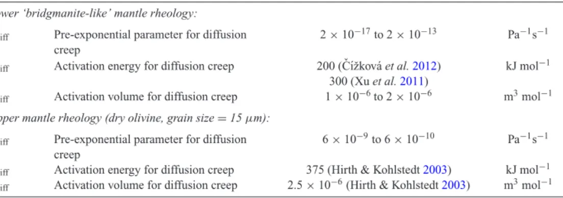
Figure 2. The different mantle viscosity profiles considered in our models for the solid phase, computed using eq. (19b). Upper panels, Ediff= 200 kJ mol−1

(with reference case highlighted in yellow) and lower panels Ediff= 300 kJ mol−1. Grey domain viscosity models from geoid inversion and post-glacial

rebound [ ˇC´ıˇzkov´a et al. (2012) and references therein]. Left-hand frame: no viscous dichotomy between the upper and lower mantle is considered. Right-hand frame: when a different upper mantle is considered. We performed calculations for Adiffand Vdiffranging from 2 × 10−17to 2 × 10−13Pa−1s−1and 10−6to

2 × 10−6_Pa−1_s−1_{, respectively (Table}₂_{). In the B-frame, we have also studied the influence of the upper mantle viscosity with A}_diff_{ranging from 6 × 10}−10

to 6 × 10−9_Pa−1_s−1_{. The viscosity profiles (red, green and blue lines) are calculated considering an adiabatic temperature profile with T}_p_{= 1600 K from the}

surface of the Earth to the CMB, thus neglecting the presence of top and bottom boundary layers for the figure readability. Table 2. Values used in eq. (19b) to calculate the solid mantle viscosity.

Lower ‘bridgmanite-like’ mantle rheology: Adiff Pre-exponential parameter for diffusion

creep 2 × 10

−17_{to 2 × 10}−13 _Pa−1_s−1

Ediff Activation energy for diffusion creep 200 ( ˇC´ıˇzkov´a et al.2012) kJ mol−1

300 (Xu et al.2011)

Vdiff Activation volume for diffusion creep 1 × 10−6to 2 × 10−6 m3mol−1

Upper mantle rheology (dry olivine, grain size = 15 µm): Adiff Pre-exponential parameter for diffusion

creep 6 × 10

−9_{to 6 × 10}−10 _Pa−1_s−1

Ediff Activation energy for diffusion creep 375 (Hirth & Kohlstedt2003) kJ mol−1

Vdiff Activation volume for diffusion creep 2.5 × 10−6(Hirth & Kohlstedt2003) m3mol−1

with αnthe coefficient in melt fraction-dependent viscosity. The

lat-ter equals 26 for deformation via olivine diffusion creep mechanism under anhydrous conditions (Mei et al.2002).

2.4 Numerical model

We model the thermal evolution of a 2900-km-thick isochemical sil-icate mantle overlying an iron core by solving for the conservation of energy (eq.1) in a 1-D, spherically symmetric domain (with a radius

ranging from 3500 to 6400 km). To this end, we used a modified ver-sion of the numerical model developed in Monteux et al. (2016). Eq. (1) is discretized using a semi-implicit predictor–corrector Finite Difference scheme, of second-order in both space and time (Press

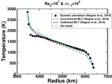
et al.1993). Our numerical scheme was successfully benchmarked against steady and unsteady analytical solutions for diffusion prob-lems (Crank1975). We have also successfully benchmarked our physical model with 3-D spherical calculations at both steady and transient states from the models developed by Wagner et al. (2019)

(8)

Table 3. Parameter values used to calculate the viscosity of the lower mantle. Viscosity layering means that we consider an upper mantle in our model.

Series # Viscosity layering Ediff(kJ mol−1) Vdiff(m3mol−1) Adiff(Pa−1s−1)

1 No 200 1 × 10−6_{–2 × 10}−6 _{2 × 10}−17_{–1 × 10}−15

2 Yes 200 1 × 10−6_{–2 × 10}−6 _{2 × 10}−17_{–1 × 10}−15

3 No 300 1 × 10−6_{–2 × 10}−6 _{5 × 10}−15_{–2 × 10}−13

4 Yes 300 1 × 10−6_{–2 × 10}−6 _{5 × 10}−15_{–2 × 10}−13

considering a relatively lower Ra number and a smaller viscosity contrast (see the Appendix). The mantle is discretized using 2900 equally spaced gridpoints resulting in a constant spatial resolution δ_{r = 1 km. The variable time step is set as δt = min(δr}2/κ(r)), where

κ(r) = k/(ρCp) is the effective diffusivity. The boundary conditions in our models are those described in Section 2.1.2: isothermal at the surface with Tsurf= 500 K and variable heat flux accounting for

heat transfer between the core and the mantle at the CMB. In all our models, the core temperature below and just above the CMB are initialized to the same value (T0,core= 4370 K).

3 . R E S U LT S : C O O L I N G A N D S O L I D I F I C AT I O N DY N A M I C S 3.1 A reference case

We followed the thermal evolution of a deep mushy ocean with an initial temperature profile corresponding to a melt fraction of 40%

throughout the whole mantle. As a reference case, we considered the chondritic-type mantle from Series 1 with Adiff= 10−15Pa−1s−1

and Vdiff= 10−6m3mol−1through the whole mantle (see Table3).

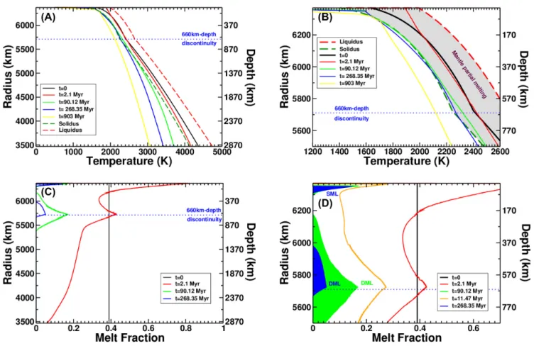
This reference case represents a lower bound in terms of viscosity (Fig.2). The temperature initially decreases rapidly from the surface where heat is efficiently extracted by conductive cooling, and where a thin TBL initially forms (Fig.3). In the deepest part of the man-tle, the temperature profile bends towards an adiabatic temperature profile, which is more vertical than the solidus profile. As a con-sequence, the solidification front starts from the lowermost mantle. After 100 Myr, most of the lower mantle temperatures lie below the solidus, nevertheless two molten reservoirs remain (named hereafter SML and DML). Fig.3(bottom panels) shows that 270 Myr after the beginning of our simulation, the deeper one (DML) is located at a depth centred at 650 km, and the depth of shallower one (SML) ranges between 20 and 60 km. Full solidification of DML occurs prior to that of SML. Finally, after 900 Myr of cooling, the entire temperature profile is below the solidus, but remains super adiabatic,

Figure 3. Upper panels: temperature time evolution as a function of depth. Lower panels: melt fraction time evolution as a function of depth. In this reference case (Series 1, Adiff= 10−15Pa−1s−1and Vdiff= 10−6m3mol−1), no dichotomy in the viscosity model is considered between the upper and lower mantle.

The blue dashed line separates the upper and lower mantle. The right-hand panels represent close-up views of the left-hand panels. When t > 90 Myr, the partially molten layer is separated in 2 layers: SML and DML.

(9)

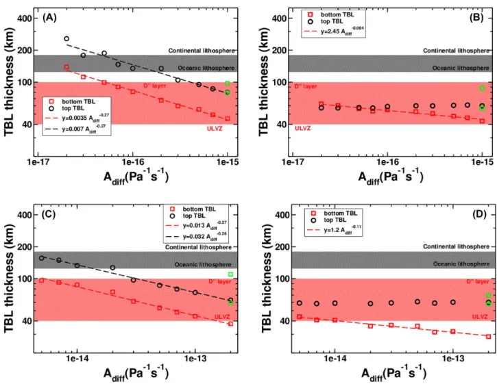
Figure 4. Thickness of the top (circles) and bottom (squares) thermal boundary layer when the mushy mantle is fully solidified as a function of Adiffand Ediff

(i.e. Ediff= 200 kJ mol−1for top figures or Ediff= 300 kJ mol−1for bottom figures). The A, B, C, D panels correspond to Series 1, 2, 3, 4, respectively

(see Tables2and3for complete set of parameter values). The cases with Vdiff= 10−6m3mol−1are illustrated with red (bottom TBL) and black (top TBL)

symbols and cases with Vdiff= 2 × 10−6m3mol−1are illustrated with green symbols. Dashed lines represent power law fits to the thermal evolution data

points.

especially in the mid-top mantle. This solidification timescale is in good agreement with the timescale proposed by Solomatov (2000), where the complete crystallization of the shallow early mantle could last more than 108_yr.

3.2 Influence of the viscosity parameters on the mushy mantle solidification

3.2.1 TBL thicknesses

From the initial thermal state, two TBLs rapidly form above and below the convecting portion of the mantle. Upon cooling, the Rayleigh number within the convecting mantle decreases and the two boundary layers thicken following the scaling used in eq. (10). Therefore, the thickness of the boundary layers scales with Ra− 1/3

and as a consequence scales with η1/3_{and A}−1/3

diff . In Fig.4, we

plot-ted both the bottom (red) and top (black) boundary layer thicknesses at the end of the mushy stage (i.e. as soon as the mantle reaches complete solidification) as a function of the viscosity exponential pre-factor (Adiff) and for two different values of the activation

en-ergy (Ediff) and activation volume (Vdiff). Our results show that the

evolution of the TBL thickness is strongly dependent on the value of the activation energy (Ediff= 200 or 300 kJ mol−1) and on Adiff

as illustrated in Fig.4. For Series 1 (Fig.4a), both the top and bot-tom boundary layer thicknesses scale with A−0.27

diff , which is close to

the theoretical scaling of A−1/3

diff for an entirely solid mantle. This

indicates that the viscosity of the solid mantle governs the thickness of the two TBL. At the end of the mushy stage, the top boundary layer thickness ranges between 80 and 250 km, whereas the bottom boundary layer thickness ranges between 45 and 140 km. For Series 3 (Fig.4c), the behaviour of the bottom TBL thickness is similar to the Series 1 cases. The bottom TBL thickness decreases as A−0.26 diff

with corresponding values ranging from ≈40 to ≈100 km, and the top TBL thickness decreases as A−0.27

diff , with corresponding values

ranging from ≈60 to ≈160 km.

When an upper mantle is considered (Figs4b and d), the influence of the lower mantle viscosity on both the top and bottom TBL thick-nesses vanishes. The bottom TBL thickness decreases as A−0.084

diff for

Series 2 and as A−0.11

diff for Series 4. For both values of Ediffwe used

for the lower mantle viscosity, the top TBL thickness decreases to a value of ≈60 km at the end of the mushy stage, independently of the value of Ediff.

(10)

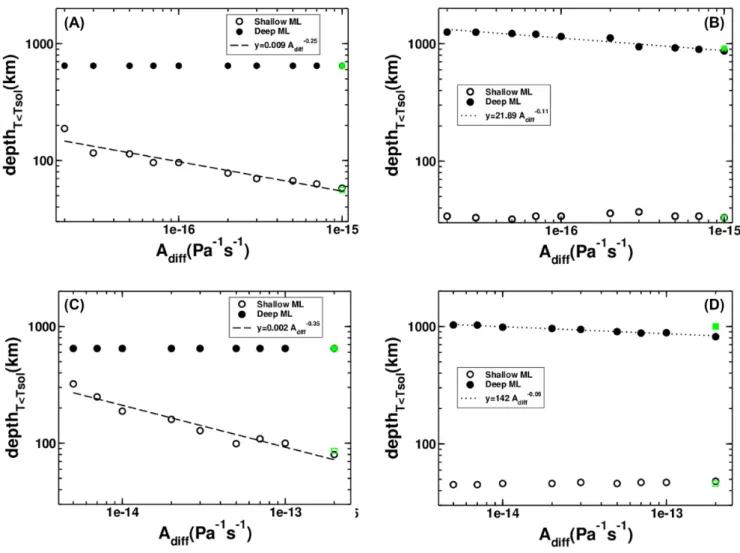
Figure 5. Depth at which the last layers of partially molten material solidify as a function of Adiff. Open symbols represent the solidification depth of the

upper molten layer (SML) whereas solid symbols illustrate the solidification depth of the lower molten layer (DML) (See also Figs3c and d). The a, b, c, d panels correspond to Series 1, 2, 3, 4, respectively (see Tables2and3for parameter values). The cases with Vdiff= 10−6m3mol−1are in black symbols

and cases with Vdiff= 2 × 10−6m3mol−1are in green symbols. Dashed and dotted lines represent power law fits of the numerical data for SML and DML,

respectively.

Also, the top TBL thickness is weakly dependent on the value of

Vdiff, as shown in Fig.4. However, this parameter strongly influences

the bottom TBL thickness. Indeed, increasing Vdifffrom 1 × 10−6

to 2 × 10−6_m3_mol−1_{results into a viscosity increase by at least}

a factor 2 to 3 for both Ediff = 200 kJ mol−1 and Ediff= 300 kJ

mol−1 _{cases, and for cases considering an upper mantle and its}

influence in rheology or not. This result illustrates the influence of

Vdiffon the viscosity, and can be understood when comparing the

red and green viscosity profiles from Fig.2. As the value of Vdiff

governs how the viscosity increases with depth from a reference value, increasing Vdiff does not change significantly the viscosity

close to the Earth’s surface. However, increasing Vdiff increases

significantly the viscosity in the lowermost mantle, leading to a significant thickening of the TBL above the core mantle-boundary. In our models, right after the solidification of the molten layers (SML and DML), the viscosity above the bottom TBL for cases with Vdiff= 2 × 10−6m3 mol−1 is larger than the viscosity above

the bottom TBL for Vdiff= 1 × 10−6m3mol−1by a factor 10–30.

This important increase in the lower mantle viscosity explains the increase in TBL thickness illustrated in Fig.4for our range of Vdiff

values as the TBL scales with η1/3_.

3.2.2 Depth of final melt layer

During the cooling and the solidification of the mushy mantle, the melt fraction decreases from a global value of 0.4 to 0 (Figs3c and d). Depending on the solid viscosity parameters used for the early mushy mantle, two layers can remain molten before full so-lidification: a deep one (DML) and a shallower one (SML, see also Fig. 3). The depths at which the two last layers of melt solidify as a function of Adifffor two different values of Ediff and Vdiffis

reported in Fig.5. This figure shows that the crystallization mech-anism strongly depends on the presence of a viscosity dichotomy between the upper and lower mantle. When no dichotomy is con-sidered (Figs5a and c), the behaviour is similar for Ediff= 200 kJ

mol−1 _{and E}_diff_{= 300 kJ mol}−1_{. For both E}_diff_{values, the}

solid-ification depth of the upper molten layer (SML) decreases as the viscosity decreases (scaling with A−0.25

diff and A−0.35diff , respectively)

whereas the solidification depth of the deep molten layer (DML) is constant and equals 660 km (i.e. the depth of the transition be-tween the upper and lower mantle). In the later case, the transition is not the consequence of rheological properties but is related to the change of the solidus slope (eqs (12a) and (12c) and Fig.3), which is steeper in the lower mantle than in the upper mantle. These

(11)

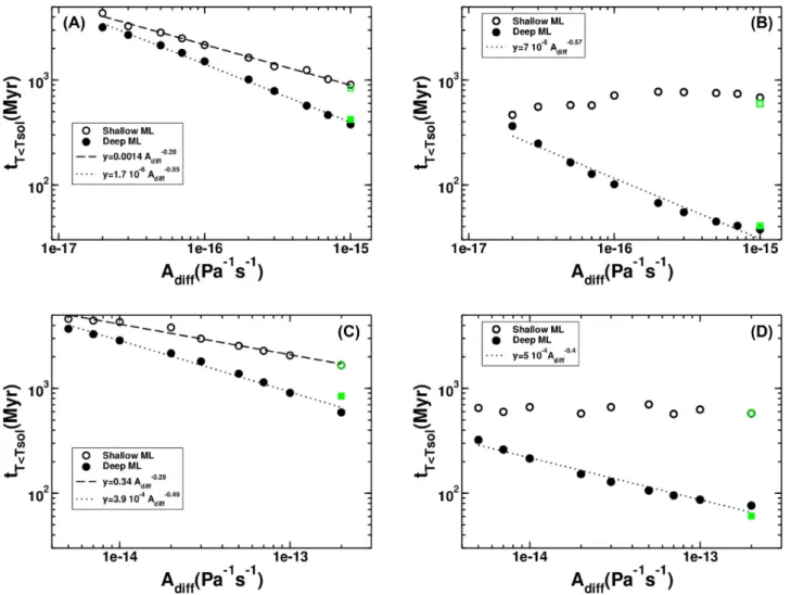
Figure 6. Duration for full solidification of the mushy mantle (initially with ϕ = 0.4). Open symbols represent the solidification time of the upper molten layer (SML) whereas solid symbols illustrate the solidification time of the lower molten layer (DML). The a, b, c, d panels correspond to Series 1, 2, 3, 4, respectively (see Tables2and3for parameter values). The cases with Vdiff= 10−6m3mol−1are illustrated with black symbols and cases with Vdiff= 2 × 10−6m3mol−1

are illustrated with green symbols. Dashed and dotted lines represent power law fits of the numerical data for SML and DML, respectively.

changes in the melting properties with depth coupled with the slope of the temperature profile computed from our models explain this particular behaviour. In these cases, the depth of the deep molten layer is insensitive to the value of the viscosity parameters.

However, a mineralogical dichotomy between the upper and lower mantle is likely to appear rapidly during the solidification of the mushy mantle, due to the high-pressure polymorphism. When con-sidering rheologically distinct upper and lower mantles (Figs5b and d), the solidification depth of the deep molten layer is no longer tied to a depth of 660 km, but now depends on the viscosity of the lower mantle. The depth at which DML solidifies decreases when Adiff

in-creases (i.e. when the lower mantle viscosity dein-creases) and scales with A−(0.06−0.1)

diff (Figs5b and d). This results in a deep solidification

stage occurring at depth decreasing from 1250 to 800 km when Adiff

increases within the range envisioned in our study (i.e. when the deep mantle viscosity decreases). In contrast, the depth of final up-per molten layer SML remains nearly constant (≈30–50 km) for the whole range of lower mantle viscosities considered in Fig.5. This illustrates the fact that the depth at which the last upper layer of melt solidifies is not governed by the viscosity of the lower mantle but rather by the rheological properties of the upper mantle (we tested this hypothesis in Section 3.2.4).

3.2.3 Mushy stage timescale

The influence of Adiffon the time required to fully solidify a

par-tially molten mantle and for two different values of Ediffand Vdiff

is reported in Fig.6. A quick inspection of eq. (1) indicates that this solidification timescale should be inversely proportional to the convective heat flux Fconv. In the hard-turbulent regime, this term

scales as η−3/7_{whereas in the soft-turbulent regime, this term scales}

as η−1/3_{. The eq. (}_19b_{) implies that an increase of either E}_diff_{or V}_diff

yields an increase of the viscosity. On the contrary, an increase of

Adiffyields a decrease of the solid viscosity at given P and T

con-ditions scaling with A−1

diff. Consequently, if the viscosity of its solid

fraction governs the characteristic solidification timescale, this time should scale as A−n

diff with n ranging between 1/3 and 3/7. This is

confirmed by our numerical results (Figs6a and c). The time re-quired for the upper molten layer (SML) to fully solidify scales with

A−0.39

diff for Series 1 (Fig.6a) and with A−0.29diff for Series 3 (Fig.6c).

For the lower molten layer (DML), the influence of mantle viscosity is even stronger and the time required for DML to fully solidify scales with A−0.55

diff for Series 1 (Fig.6A) and with A−0.49diff for Series

3 (Fig.6c).

When no upper/lower mantle dichotomy is considered, the du-ration of the complete mushy mantle solidification ranges between

(12)

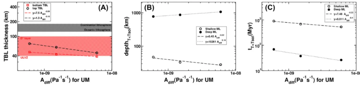
Figure 7. TBL thickness (a), depth at which the last layers (upper and lower) of partially molten material solidify (b) and time to fully solidify the last layers (upper and lower) of partially molten (c) as a function of the value of Adiffin the upper mantle. In these figures, Adiff= 10−15Pa−1s−1, Ediff= 200 kJ mol−1

and Vdiff= 10−6m3mol−1in the lower mantle whereas Ediff= 375 kJ mol−1and Vdiff= 2.5 × 10−6m3mol−1in the upper mantle. Open symbols represent

the solidification time of the upper molten layer (SML) whereas solid symbols illustrate the solidification time of the lower molten layer (DML). Dashed and dotted lines represent power law fits of the numerical data for SML and DML, respectively.

900 Myr and 4.4 Gyr for Series 1 (Fig.6a). For Series 3 (Fig.6c), the solidification duration ranges between 1.6 and 4.6 Gyr. Our results also show that the solidification of the deeper DML occurs prior to that of the shallower SML, with times ranging between 375 Myr and 3.2 Gyr for Ediff= 200 kJ mol−1or between 590 Myr and 3.7 Gyr

for Ediff= 300 kJ mol−1. Fig.6also shows that our solidification

timescale is nearly insensitive to the value of Vdiff.

When considering an upper mantle rheologically different from the lower mantle (Figs6b and d), several changes occur, compared to models without viscous dichotomy. The solidification timescale for the upper molten layer (SML) is less affected by changes in the value of Adiffthan DML. Thus, the time required to fully solidify

the whole mantle (SML and DML) exhibits a narrower range of values (between 460 and 770 Myr for Series 2 and between 570 and 700 Myr for Series 4). On the contrary, the solidification time of the deeper molten layer DML strongly depends on the viscosity of the lower mantle and scales with A−0.57

diff for Series 2 and with

A−0.4

diff for Series 4. Again, the solidification time of DML is faster

than SML (between 37 and 365 Myr for Series 2 or between 76 and 322 Myr for Series 4). Our results suggest that the solidification of the SML (i.e. the final episode of solidification of the early mantle in our models) is weakly sensitive to the viscosity of the lower mantle but is mostly governed by the viscosity of the upper mantle. On the other hand, the solidification time of the DML is in comparison faster, and the viscosity of the lower mantle governs the time delay. This is certainly related to the relatively low upper mantle viscosity used in this calculation (see Fig.2).

3.2.4 Influence of the upper mantle viscosity

We then investigated the influence of the upper mantle viscosity on the characteristic time and length scales of mushy terrestrial mantle crystallization. Thus we considered the reference case detailed in Fig.3with a dichotomy in the viscosity between the upper and lower mantle. In this section, we consider constant values for Adiff, Ediff

and Vdifffor the lower mantle, and we used three different values for

Adifffor the upper mantle ranging between 6 × 10−10and 6 × 10−9

Pa−1_s−1_.

The results given in Fig.7show that the viscosity of the upper mantle influences both the shallow characteristic time and length scales. We recall here that increasing the value of Adiffresults in

a viscosity decrease. Fig. 7(a) shows that both the top and the bottom TBL thicknesses now decrease when Adiffin the upper mantle

increases. The top TBL is more sensitive to variations in the Adiff

values in the upper mantle than the bottom TBL (power exponent –0.19 compared to –0.9 in top and bottom TBL, respectively). In Fig. 7(b), the results show that the depth at which the shallow molten layer SML solidifies decreases with A−0.22

diff , whereas the

depth at which the deep molten layer DML solidifies increases with

A0.14

diff. This means that decreasing the upper mantle viscosity (i.e.

increasing Adiffin the upper mantle) favors a deeper solidification

of DML, while favoring the solidification of SML closer to the surface. Finally, results from Fig.7(c) shows that both the time at which SML and DML solidify decrease when increasing Adiffin the

upper mantle. Interestingly, the viscosity of the upper mantle has a stronger influence on the solidification time for the DML than on the shallow SML (power exponent –0.4 compared to –0.22). Hence, by controlling the heat loss in the shallower part of the early Earth, the upper mantle viscosity strongly influences the characteristic solidification time and length scales.

Figs 5(b), (d) and 6(b), (d) show that, when a dichotomy in viscosity is considered, the depth and solidification time of the shallow molten layer are weakly dependent on the viscosity of the deep mantle. However, Fig. 7illustrates that the viscosity of the upper mantle plays a key role on the time and depth of solidification of the shallow molten layer and is more important than the influence of the lower mantle on this time. Concerning the DML, a decrease of either upper or lower mantle viscosity leads to a decrease of the solidification time of this layer. Nevertheless, this time is more influenced by the viscosity of the deep mantle than by the viscosity of the upper mantle (power exponent –0.57 compared to –0.4). An interesting behaviour arises from the depth at which the deep molten layer DML solidifies. Indeed, Figs5(b)–(d) shows that this depth decreases when Adiffin the lower mantle increases (i.e. when the

viscosity decreases) for a fixed value of Adiffin the upper mantle. On

the contrary, the depth at which DML solidifies increases when Adiff

in the upper mantle increases for a fixed value of Adiffin the lower

mantle. Our results show that the rheological parameters of both the upper and lower mantle govern the deep processes of solidification in the lower mantle, whereas the shallower solidification processes are governed only by the properties of the upper mantle.

3.2.5 Summary

We have developed a numerical approach to constrain the charac-teristic depth and time of solidification of a mushy mantle. We have identified two persistent molten layers (SML) and (DML). We show that the cooling and solidification dynamics are very sensitive to the

(13)

Rayleigh number that increases with decreasing viscosity. Hence, an increase of the pre-exponential factor Adiff(i.e. a decrease of the

viscosity) systematically leads to a decrease of the TBL thicknesses (in agreement with eq.10) and as a consequence to the depth of so-lidification of the last layer of molten material. As higher Ra values lead to a more efficient cooling of the early mantle, the timescale of complete solidification of the mantle also decreases with de-creasing Adiff. Within a moderately convecting viscous mantle, the

TBL thickness and the cooling timescale are expected to scale with

Ra− 1/3_{while within a turbulent reservoir they are expected to scale}

with Ra− 2/7_{. In our models were important changes in the}

param-eters occur with temperature, pressure and melt fraction, the value of the exponent in the power law is slightly different (from –0.25 to –0.55 when no viscous dichotomy is considered) but the behaviour is similar.

We have characterized the influence of the solid mantle viscosity with or without a rheological contrast between the upper and lower mantle. Our parametrical study shows that the viscosity of the deep mantle influences the solidification of the DML. This result is not surprising since the bottom TBL thickness is related to the viscosity of the deep material. Hence, one can expect that the solidification characteristics (depth and time scales) of the DML to be strongly influenced by the values of Adiffin the lower mantle. Our results

show that the same reasoning can be applied to the solidification characteristics of the SML that is governed by the values of Adiffin

the upper mantle.

Our results show that the viscosity of the upper mantle affects the DML solidification characteristics. This feature illustrates that the upper mantle governs the global mantle dynamics by acting as a thermal blanket that reduces the efficiency of heat loss. Hence, a decrease in the upper mantle viscosity leads to an increase of the surface heat flux, to a more vigorous internal convection associated with a thinner bottom TBL (Fig.7a), and to a more rapid solid-ification (Fig.7c). Conversely, the viscosity of the lower mantle does not influence significantly the SML solidification character-istics (Figs4–6, right-hand panels). Again, this illustrates that the viscosity of the upper mantle mostly controls the cooling and solid-ification dynamics. A low viscosity lower mantle enhances the heat transfer from the core toward the mantle but the mantle heat loss is limited by the viscous properties of the upper mantle.

4 . D I S C U S S I O N 4.1 Geological constraints

A mineralogical dichotomy and a subsequent transition of the vis-cous behaviour between the upper and lower mantle are likely to appear rapidly during the solidification of the mushy mantle. In the following discussion we only consider the results from the models that account for a viscous dichotomy between the upper and lower mantle (i.e. left-hand column, b and d graphics in Figs4–6). Our model results show that the top melt layer (SML) crystallizes at the Hadean-Eoarchean boundary (500–800 Myr after Earth’s for-mation; Fig. 6), regardless of the model, and the crystallization proceeds at relatively shallow depths of 35–45 km (Fig.5). On the contrary, the bottom melt layer (DML) crystallizes at deeper lev-els (800–1000 km; Fig.5) and earlier (40–400 Myr after Earth’s formation; Fig.6). If the upper mantle viscosity is considered sep-arately, these time and depth estimates are only slightly decreased or increased (Fig.7).

The presence of molten material and the resulting rheologi-cal weakening may have profound effect on the evolution of the early crust, on its ability to deform and on how orogens develop (Sawyer et al.2011). The persistence of a melt layer at shallow depth during the Hadean and its final crystallization around the Hadean–Eoarchean boundary could prevent the formation of el-evated orogenic formations due to fast isostatic compensation of any created reliefs and development of large-scale tectonic fault and shear-zones. The absence of reliefs would, in turn, result in a water-world with most of the Earth being covered by shallow water. Major faults and shear-zones could represent pathways for liquid water to penetrate to lower crustal levels and, in turn, induce intense hydrothermal activity. In addition, this weak layer at the depth of the lower crust could possibly isolate the crust from the underlying mantle. Doglioni et al. (2011) proposed that a stable partial melt layer between the asthenosphere and the lithosphere could induce an effective viscous decoupling between the two layers and explain the lifetime of cratonic roots. At the Hadean–Eoarchean, the viscous coupling between the mantle and the crust could have induced the beginning of large-scale Hadean crust reworking and the formation of stable Archean crustal blocks. The persistence of SML could, hence, account for the absence of Hadean crustal fragments in geo-logical record and at the beginning of the Archean geogeo-logical record. They are solid outputs from our geodynamic models and, therefore, they should have affected the dynamics of our planet early in its history. Hence, linking the timing of major differentiation events in the geological record with SML and DML crystallization could help understanding early shallow processes.

Little is known about the Hadean period since we do not have the rock record at the Hadean–Eoarchean boundary (e.g. Good-win1996; Guitreau et al.2012). Yet, some detrital zircon crystals, formed during the Hadean, survived until today. They offer a win-dow into the Earth’s infancy (e.g. Froude et al.1983; Cavosie et al. 2019). In addition, relics of global chemical fractionation that oc-curred during the Hadean are recorded by extinct radionuclides, such as142_{Nd and}182_{W (e.g. Boyet et al.} ₂₀₀₃_{; Touboul et al.}

2012). The 182_Hf-182_{W system operated during the first 50 Myr}

after Solar System formation, and it is, hence, unlikely to have recorded processes depicted in our model. In contrast, the lifetime of146_Sm-142_{Nd system matches very well the timescale for DML}

crystallization and is, hence, very appropriate to help constrain the physical parameters of our models. Interestingly, most142_Nd

sig-natures point to major differentiation event(s) of the Earth around 4.3–4.4 Ga (i.e. 150–250 Ma after the Earth’s formation, e.g. Saji

et al.2018, and references therein, Guitreau et al.2019), also con-sistent with detrital zircon ages (e.g. Cavosie et al.2019). On the other hand, the disappearance of SML would correspond to the start of the rock record (i.e. preservation of stable crustal blocks) between 4.0 and 3.8 Ga.

Considering that the SML crystallization is correlated with the end of major resurfacing on Earth, the comparison with Venus is quite appealing. Based on the crater population, it was suggested that the surface of Venus seems uniformly young. With absence of plate tectonics, this observation suggested that catastrophic resurfacing occurs episodically on Venus (Phillips & Hansen1998; Harris & B´edard2014; Smrekar et al.2018). The available geodynamic mod-els point out the importance of radioactive heating in the Venusian mantle which, correlated to the presence of a rigid stagnant lid, could have resulted in an increase of the mantle potential tempera-ture with geological time, especially in the first 1–2 Ga (O’Rourke & Korenaga2012; Tosi et al.2017). The mantle potential temper-ature could still be today above 1800 K on Venus, thus at a similar

(14)

Figure 8. For the lower mantle, range of Adiffvalues considered in our study for (left-hand panel) Ediff= 200 kJ mol−1and (right-hand panel) Ediff= 300 kJ

mol−1_{. The grey domain marks dislocation creep regime, below is diffusion creep regime. The white domains represent A}_diff_{values not considered in our study.}

The red dashed domains on the colour bar represent the values derived from the geological constraints.

level than it was early in the Earth’s history (e.g. Herzberg et al. 2010). A logical conclusion is that partial melting still takes place today at shallow depths in the Venusian mantle.

4.2 Refinement of mantle’s rheological parameters

Following the idea that SML and DML final crystallization cor-respond to identified Hadean geological events on Earth, the ex-act timing of these events can help refine most realistic values of

Adiff, Ediffand Vdiff. In our models, the upper mantle viscosity does

not significantly influence the solidification time of the last global molten layers, and should not strongly affect the timing of the geo-logical events discussed above. We cannot estimate the best pair of

Ediffand Vdiff, since Vdiffhas very little influence on the timing of

crystallization of SML and DML. Nevertheless, we can propose a couple of solutions for fixed values of Ediff. SML crystallization is

essentially insensitive to Adiffvalues and we, hence, cannot use it to

estimate Adiffvalues. On the other hand, the crystallization of DML

is sensitive to Adiffvalues. In order to explain the ages of 4.3–4.4 Ga

inferred form142_{Nd signatures, the lower mantle A}

diffvalues should

range between 3 × 10−17_{and 7 × 10}−17_Pa−1_s−1_{for Series 2, and}

7 × 10−15_Pa−1_s−1_{to 2 × 10}−14_{for Series 4. Assuming that SML}

accounts for the start of the geological record (i.e. preservation of stable crustal blocks) between 4.0 and 3.8 Ga, the upper-mantle Adiff

values should range between 1 × 10−9_{and 4 × 10}−9_Pa−1_s−1_{. These}

ranges of values obtained for Adiffin the lower and upper mantle are

pretty narrow given that reference viscosities are generally unknown to multiple orders of magnitude. Moreover, the values inferred for both the lower and the upper mantle are within the range of those proposed for the mantle ( ˇC´ıˇzkov´a et al.2012).

4.3 Chemical weakening and grain size

Among the parameters used to compute the solid-state mantle vis-cosity the pre-exponential factor exhibits a large range of plausible values (typically two orders of magnitude). While Adiffis called the

material constant, its variability expresses the grain size sensitivity and the potential influence of chemical weakening. For olivine, this influence has been experimentally characterized for hydrogen at crustal and upper mantle pressures (e.g. Mackwell et al.1985; Mei & Kohlstedt2000a,b, Demouchy et al.2012; Girard et al.2013; Tielke et al.2017), for iron (Zhao et al.2009; Hansen et al.2012),

and for titanium, (Faul et al.2016). It can be expressed as:

1 Adi f f = 2 !_{A A}′ C W′ µ "−1!_b d "−3 , (20)

where A is thus a material constant (A = 8.17 × 1015 _s−1_{), µ is}

the shear modulus (µ = 80 GPa), b is the magnitude of the Burg-ers vector (b = 0.55 × 10−9 _{m) and d is the grain size (Karato}

& Wu1993). A′

C W is a dimensionless parameter characterizing the

influence of the potential chemical weakening due to the incorpo-ration of, for example Al3+_{, Fe}2+/3+_{, Ti}4+_{in mantle minerals. A}′

C W

can be envisioned as a stress factor in the sense that an increase of its value leads to an increase of Adiffand, as a consequence, to

a viscosity decrease. Note that hydrogen is expected to have only very minor to negligible effect on lower mantle properties, since hydrogen can barely be embedded in bridgmanite as a point defects (Bolfan-Cavanova, Keppler & Rubie2003) and since the hydrogen solubility in periclase remains very limited (Bolfan-Casanova et al. 2002, see Bolfan-Casanova2005, for a review). Therefore, ‘water’ weakening in the lower mantle is discarded in this study.

In our models, we have considered different values for Adiff

rang-ing between 2 × 10−17_Pa−1_s−1_{and 10}−15_Pa−1_s−1_{for E}

diff= 200 kJ

mol−1_{and between 5 × 10}−15_Pa−1_s−1_{and 2 × 10}−13_Pa−1_s−1_for

Ediff= 300 kJ mol−1. According to eq. (20), each value of Adiff

corresponds to a set of values for the pair d and A′

C W. In Fig.8,

we plotted Adiffas a function of d and A′C W. From Fig.8, we can

estimate the range of plausible values for d and A′

C W corresponding

to the values of Adiffconsidered in our models. The transition from

diffusion to dislocation creep is expected to occur for d larger than 100 µm in the lower mantle (Boioli et al.2017). Considering only a domain where the diffusion creep scaling applies, Fig.8illustrates that d ranges between 10 and 100 µm for Ediff = 200 kJ mol−1

and between 1 and 100 µm for Ediff= 300 kJ mol−1. In the mean

time, A′

C W ranges between 10−7and 10−4for Ediff= 200 kJ mol−1

and between 10−7_{and 10}−2_{for E}_diff_{= 300 kJ mol}−1_{. Fig.}₈_shows

that when increasing the grain size by a factor 10, the stress factor associated to chemical weakening has to be increased by a factor 1000 to maintain a constant pre-exponential factor Adiff.

Our arguments developed in previous sections suggest the follow-ing range for Adiffvalues within the lower mantle: between 3 × 10−17

and 7 × 10−17 _Pa−1_s−1 _{for E}_diff _{= 200 kJ mol}−1_{, and between}

7 × 10−15_Pa−1_s−1_{and 2 × 10}−14_Pa−1_s−1_{for E}_diff_{= 300 kJ mol}−1_,