HAL Id: hal-00330094
https://hal.archives-ouvertes.fr/hal-00330094
Submitted on 21 Nov 2006
HAL is a multi-disciplinary open access
archive for the deposit and dissemination of
sci-entific research documents, whether they are
pub-lished or not. The documents may come from
teaching and research institutions in France or
abroad, or from public or private research centers.
L’archive ouverte pluridisciplinaire HAL, est
destinée au dépôt et à la diffusion de documents
scientifiques de niveau recherche, publiés ou non,
émanant des établissements d’enseignement et de
recherche français ou étrangers, des laboratoires
publics ou privés.
Distributed under a Creative Commons Attribution - NonCommercial| 4.0 International
License
Assigning the causative lightning to the whistlers
observed on satellites
J. Chum, F. Jiricek, O. Santolik, Michel Parrot, G. Diendorfer, J. Fiser
To cite this version:
J. Chum, F. Jiricek, O. Santolik, Michel Parrot, G. Diendorfer, et al.. Assigning the causative lightning
to the whistlers observed on satellites. Annales Geophysicae, European Geosciences Union, 2006, 24
(11), pp.2921-2929. �10.5194/angeo-24-2921-2006�. �hal-00330094�
www.ann-geophys.net/24/2921/2006/ © European Geosciences Union 2006
Annales
Geophysicae
Assigning the causative lightning to the whistlers observed on
satellites
J. Chum1, F. Jiricek1, O. Santolik1,2, M. Parrot3, G. Diendorfer4, and J. Fiser1
1Institute of Atmospheric Physics, Bocni II/1401, 14131 Prague, Czech Republic
2Charles University, Faculty of Mathematics and Physics, V Holesovickach 2, 18000 Prague, Czech Republic 3LPCE/CNRS, 3A Avenue de la Recherche Scientifique, 45071 Orl´eans, France
4Austrian Electrotechnical Association (OVE-ALDIS), Kahlenberger Str. 2A, 1190 Vienna, Austria
Received: 11 July 2006 – Accepted: 6 September 2006 – Published: 21 November 2006
Abstract. We study the penetration of lightning induced
whistler waves through the ionosphere by investigating the correspondence between the whistlers observed on the DEMETER and MAGION-5 satellites and the lightning dis-charges detected by the European lightning detection net-work EUCLID. We compute all the possible differences be-tween the times when the whistlers were observed on the satellite and times when the lightning discharges were de-tected. We show that the occurrence histogram for these time differences exhibits a distinct peak for a particular character-istic time, corresponding to the sum of the propagation time and a possible small time shift between the absolute time as-signed to the wave record and the clock of the lightning de-tection network. Knowing this characteristic time, we can search in the EUCLID database for locations, currents, and polarities of causative lightning discharges corresponding to the individual whistlers. We demonstrate that the area in the ionosphere through which the electromagnetic energy in-duced by a lightning discharge enters into the magnetosphere as whistler mode waves is up to several thousands of kilome-tres wide.
Keywords. Ionosphere (Ionosphere-atmosphere interac-tions; Wave propagation) – Meteorology and atmospheric dynamics (Lightning)
1 Introduction
Whistlers were first observed on the Earth as whistling sounds of unknown origin heard on long-distance telephone lines, and they were, for the first time, unambiguously re-ported by Barkhausen (1919). Based mainly on the observa-tion that whistlers sometime followed impulsive
atmospher-Correspondence to: J. Chum
ics, Barkhausen (1930) put forward the theory that they are associated with lightning discharges. Eckersley (1935) for-mulated the mathematical expression for the dispersion of whistlers. The detailed explanation was developed by Storey (1953), who showed that whistlers originate in normal impul-sive atmospherics which travel through the ionosphere and magnetosphere, following the magnetic field lines and cross-ing the equator at a great height, and arrivcross-ing to the ground at a magnetically conjugate point on the opposite hemisphere. During their journey they become dispersed, so as to arrive as whistling tones decreasing in frequency – “whistlers”. Their dispersion is consistent with the right-hand polarised plasma waves propagating at frequencies both below the electron cyclotron frequency and below the plasma frequency. The whole branch of these plasma waves is now called whistlers or whistler-mode waves. The origin of whistler mode waves observed in the ionosphere and magnetosphere is not always connected with lightning discharges. In this paper, we will use the term whistlers only for waves that originate in light-ning discharges. A significant contribution to the investi-gation of the propainvesti-gation of whistlers in the magnetosphere was later done by Helliwell (1965). Since the dispersion of whistlers depends on the plasma density, measurements of whistler dispersion were used to deduce the electron/plasma density profile in the magnetosphere.
New possibilities in whistler investigation emerged with the era of artificial satellites. The wave measurements by satellites showed a much higher occurrence rate of whistlers than was observed on the ground, and revealed other types of lightning induced whistlers that are not observable on the ground. Gurnett and Shawhan (1965) presented and ex-plained ion cyclotron whistlers. These are observed on the frequency-time spectrograms as a tone which starts immedi-ately after the reception of a fractional-hop whistler (whistler with low dispersion that did not yet cross the equator). Af-ter an initial rapid rise in frequency, these waves asymp-totically approach the proton cyclotron frequency. Smith
2922 J. Chum et al.: Assigning the causative lightning to the whistlers observed on satellites and Angerami (1968), using measurements on OGO 1 and
OGO 3 satellites, first reported Magnetospherically Reflected (MR) whistlers predicted by Kimura (1966). The MR whistlers are highly oblique (with respect to magnetic field lines) propagating waves that undergo a reflection in the re-gion where their frequency is close to the local Lower Hybrid Resonance (LHR) frequency. Thus, the highly oblique prop-agating MR whistlers could not be observed on the ground. To become sufficiently oblique, the waves have to travel a rel-atively long trajectory, which means that they have to cross the equator. Additionally, there should be no distinct field-aligned density gradients that ensure the so-called ducted or field-aligned propagation, which prevents the magnetospher-ical reflection. The ducted whistlers that reach the iono-sphere may penetrate through and be received at the ground. Note that only the whistler waves having a small wave nor-mal angle with respect to the vertical direction can transform into “free space” mode because the refractive index in the non-ionised atmosphere is ∼1, which is much lower than the refractive index of whistlers in plasma medium. All other waves are reflected from the bottom-side of the ionosphere. Thus, the best conditions for the whistlers to penetrate the ionosphere and to arrive at the ground are at higher latitudes, where the magnetic field lines are approximately vertical. In-deed, Manoranjan et al. (1974) reported the low-latitude cut-off for whistlers observed on the ground, despite the fact that most of the lightning activity is in the tropics and/or in the subtropics (see, e.g. Rycroft et al., 2000).
Besides the new phenomena, the satellite and rocket mea-surements also brought the possibility to compare measure-ments on the satellites with measuremeasure-ments carried out on the ground and to measure the wave normal directions in the top-side ionosphere. The measurements of wave normal angles can either be performed for downgoing waves or for upgo-ing waves. Wave normal angles of downgoupgo-ing waves were investigated, for example, by Iwai et al. (1974), using mea-surements on the K-9M-41 rocket at heights between 130 and 270 km. These measurements were performed at rela-tively low latitudes. They also correlated whistlers recorded on the rocket with whistlers observed at ground stations lo-cated at 24◦N and 20◦N of geomagnetic latitudes. They showed that the wave normal angles with respect to the mag-netic field were mostly between 20◦ and 50◦, and the wave normal angles of whistlers observed simultaneously on the ground were small with respect to the vertical. Regarding the upgoing waves, these are strongly refracted when they enter the base of the ionosphere, and their wave normal angles are brought close to the vertical in the maximum of the ionisa-tion, due to a rapid increase in the refractive index. In the topside ionosphere, the wave normal vectors can be signifi-cantly diverted from the vertical, due to large-scale density gradients, as was shown by James (1972). The large-scale density gradients are present mainly in the mid-latitude iono-sphere. Most of the upgoing fractional-hop whistlers seem to be unducted (Hughes and Rice, 1997). The whistler-mode
waves might also be scattered from small-scale, field-aligned plasma density irregularities. Bell and Ngo (1990) showed that this scattering may lead to the excitation of electrostatic LHR waves.
The whistler waves have also been studied due to their in-fluence on radiation belt electrons, owing to wave particle interactions (Kennel and Petchek, 1966; Brinca, 1972; Abel and Thorne, 1998a, 1998b, etc.). The overall significance of lightning-generated whistlers to inner radiation belt elec-tron loss rates is still an open question, and the approach to the problem and published results of various authors differ in some details. Rodger et al. (2003) assumed ducted propaga-tion and concluded that whistler-induced electron precipita-tion dominates in the L-shell range with L=2–2.4. Lauben et al. (2001) and Bortnik et al. (2003) assumed obliquely prop-agating and MR whistlers. They came to the conclusion that the whistler energy in the magnetosphere has a flat peak at L∼2.8, and argue that obliquely propagating whistlers may be responsible for the formation and maintenance of the slot region in the electron radiation belt, a subject studied previ-ously by many authors (see, e.g. Lyons et al., 1975; Imhof et al., 1986; Abel and Thorne, 1998a, b, and references therein). All these authors had to deal with an estimation of the area through which the lightning energy enters the mag-netosphere.
The electromagnetic waves generated by a lightning dis-charge propagate away from the source within the Earth-ionosphere waveguide. An interesting experimental evidence of this propagation are “tweek” atmospherics, which exhibit remarkable dispersions near the cutoff frequencies of the first and higher modes of the Earth-ionosphere waveguide (Yamashita, 1978; Hayakawa et al., 1994, and references therein). At the bottom-side ionosphere a portion of the energy of atmospherics leaks upwards into the ionosphere where it starts to propagate in the whistler mode. The ef-fectiveness of this leakage and transformation to the whistler mode depends on ionospheric conditions.
Despite the relatively long history of the investigation of whistlers, there is a lack of information on the effectiveness of the free-space mode to the whistler mode conversion and on the size of the area in the ionosphere in which this con-version takes place. In this study, we will try to estimate the characteristic area through which the lightning energy enters the magnetosphere. We will use observations of fractional-hop whistlers on satellites. We will compare the times of the whistler arrivals to the satellite with the times of lightning discharges detected by the ground-based lightning detection network. We will show that it is possible, with high proba-bility, to find causative lightning discharges to the observed fractional-hop whistlers. In a statistical approach, we are able to estimate the area in which the free-space lightning induced electromagnetic waves transform to whistler mode waves and enter the magnetosphere.
2 Experimental data
In the following, we will give a short description of the ex-perimental data used in the analysis. These are data from the ground-based lightning detection network and satellite mea-surements of one component of the electric field in the VLF frequency range.
2.1 The lightning detection network EUCLID
EUCLID (EUropean Cooperation for LIghtning Detection) is a collaboration among national lightning detection net-works with the aim to identify and detect lightning all over the European area. Operation of the EUCLID network started in 2000 and currently, the complete EUCLID network consists of 125 sensors contributing to the detection of light-ning.
All the lightning data are detected by means of elec-tromagnetic sensors in the LF frequency range (10 kHz– 350 kHz), which send raw data to a central analyzer. The technology involved is provided by Vaisala (Tucson, AZ). Each sensor detects the electromagnetic signal emitted by the lightning return stroke, and GPS satellite signals are used for precise time stamping. For each lightning stroke, the main parameters are calculated and recorded, namely the time of the event, the impact point (latitude and longitude), the peak current and polarity. As in the NLDN (National Lightning Detection Network) in the United States, strokes are grouped into flashes using a spatial and temporal clustering algorithm (Cummins et al., 1998). The data of all the sensors through-out the network are processed in two Euclid central oper-ational centres and provide a complete picture of lightning activity in real time. In parallel, data are archived for post-storm analysis, as used in this study.
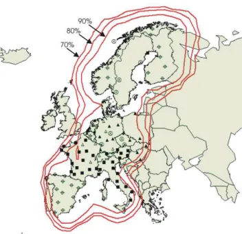
The operation of EUCLID started in 2000, and since that time the network has undergone several extensions by in-tegrating additional national networks, sensor upgrades and hence the detection efficiency and area of coverage of the EUCLID network has increased over the years. A model-based projection of the EUCLID network detection effi-ciency is shown in Fig. 1. Note that the detection effieffi-ciency falls off rapidly as the sea coast and borders are approached, as a result of a lack of sensors.
The type of sensors employed in the EUCLID network (IMPACT, LPATS) and the configuration setting of the EU-CLID central processor are primarily designed for best per-formance in detecting cloud to ground lightning (CG). Only a small fraction (a few percent) of intra/intercloud (IC) dis-charges is detected by EUCLID, and detection efficiency of IC is not uniform across the area of coverage.
The output format of the lightning data used in our anal-ysis contains the times of the detected lightning strokes in a millisecond resolution, location of these lightning strokes (geographic latitude and longitude), peak current estimate
Fig. 1. Projected Flash Detection Efficiency for the EUCLID Net-work (NetNet-work status October 2005) for peak currents greater than 5 kA.
(including the polarity), and information about the lightning type (CG or IC discharges).
2.2 Satellite VLF data, and the whistler time determination In our analysis, we have used data from two satellites: DEMETER and MAGION-5. DEMETER is a French satel-lite launched at the end of June 2004, and orbiting at an altitude of about 710 km along approximately a circular or-bit with an inclination of 98.3◦. We use the waveform of one component of the electric field measurement in the VLF frequency range by the ICE experiment (Berthelier et al., 2006). The waveform is available when the satellite is in the burst mode. The sampling frequency is fs=40 kHz. The data are transmitted to the Earth in digital form. MAGION-5 was a Czech satellite that was in regular operation from June 1998 to July 2001. It orbited at a highly elliptical or-bit with perigee ∼1200 km and apogee ∼19 000 km, with an inclination of 63.3◦. VLF data transmitted to the Earth in analogue form were recorded and digitised with a sampling frequency of fs=44.1 kHz. The analysed data cover altitudes from ∼3000 km to ∼7000 km.
Detailed frequency-time spectrograms were computed from the waveforms. To obtain a high frequency-time reso-lution, a waveform was multiplied by a Gaussian window in the time domain before computing Short Time Fourier Trans-form (STFT) using an FFT algorithm. We use the 7/8 over-lapping of the time intervals on which the FFT is applied. Thus, in the case of a 4096-point FFT, one column in the spectrogram represents a ∼512/fs∼12 ms time interval.
2924 J. Chum et al.: Assigning the causative lightning to the whistlers observed on satellites
Fig. 2. Lightning discharges and the magnetic footprints of the MAGION-5 satellite from 00:15 UT to 00:35 UT on 5 June 2000. Circles (blue) correspond to −CG discharges, crosses (red) to +CG discharges and asterisks (green) to IC discharges.
We have manually (by eye) searched for the fractional-hop whistlers on detailed spectrograms. Since the disper-sion of fractional-hop whistlers is low, we have not evaluated it. We determine the time of whistler arrival at the satel-lite by “clicking” the data cursor on individual fractional-hop whistlers at the frequency of 5 kHz in the electronic version of spectrograms.
2.3 Example of lightning activity-satellite orbit configura-tion
To characterize the position of a satellite with respect to the lightning discharges, we trace the satellite position along the magnetic field line to the bottom of the ionosphere, where we stop the tracing at an altitude of 110 km. We will call these points magnetic footprints of the satellite from now on. Fig-ure 2 shows a sequence of magnetic footprints along the orbit of Magion-5 satellite, and the locations of detected lightning discharges by the EUCLID network. Different types of light-ning discharges are distinguished by different symbols. Note that if during a given satellite pass the magnetic footprints do not cross the centre of the lightning activity and/or the lightning activity is located on one side of the line of the footprints, then this satellite pass does not cover all possible distances and azimuths between the magnetic footprints and the locations of the lightning at the times corresponding to the individual flashes.
3 Data processing and obtained results
In order to find the correspondence between the whistlers ob-served on the satellites and the lightning discharges detected by the ground-based EUCLID network, we have computed a matrix containing all the possible differences twi−tlj, where twiis the time of the i-th detected whistler (i=1..M), and tlj is the time of the j -th detected lightning discharge (j =1..N) in the analysed time interval. The length of the analysed time interval depends on the orbit of the given satellite, and it is about 5 min for DEMETER satellite and about 20 min in the case of the MAGION-5 satellite. It can also be limited by the length of the VLF record, e.g. by the length of the burst mode on the DEMETER satellite. Note that the number of detected whistlers M is usually different from the number of detected lightning discharges N . If predominantly the whistlers corresponding to the lightning discharges detected by the EUCLID network arrive at the satellite, we can ex-pect that a certain narrow interval of time differences will occur most frequently in the matrix. These time differences would correspond to the propagation time of the waves from the discharges to the satellite and to a possible small time shift between the clock used by the EUCLID network and the clock used in the VLF record. We suppose this time shift between the clocks to be constant during the analysed time interval, which is obviously true. Concerning the propaga-tion times from the discharges to the satellite, we suppose that they do not change significantly for 5-kHz waves dur-ing the analysed part of the orbit. This is true for the ob-servation of fractional-hop whistlers by DEMETER. In the case of MAGION-5, small differences in propagation times comparable with the time resolution of whistler detection are observed when we divide the analysed part of the orbit into several time intervals (not shown). This variation of propa-gation time is caused both by the variation of length of the wave trajectory and by variation of whistler dispersion. The change in the whistler dispersion along the orbit was stud-ied in more detail by Hughes (1981), and Hughes and Rice (1997), who measured the dispersion on the ISIS-2 satellite at an altitude of ∼1400 km and showed that the dispersion varies from ∼5 s1/2at a magnetic latitude of 25◦to ∼12 s1/2 at the equator. Since our observations concern middle lati-tudes, these variations are negligible in our case.
In the next step, we construct an occurrence histogram of time differences twi−tlj in the matrix. It is convenient to do it only for reasonable time differences. We have constructed the occurrence histogram with a time step of 25 ms. Two examples of these histograms are presented in Figs. 3 and 4. Different symbols distinguish various types of lightning discharges. The curve corresponding to the highest occur-rence rate represents all types of lightning. Figure 3 stands for MAGION-5’s orbit during the nighttime conditions on 5 June 2000; the map with lightning activity and satellite orbit was presented in Fig. 2. Figure 4 shows the results for the orbit of the DEMETER satellite during daytime conditions
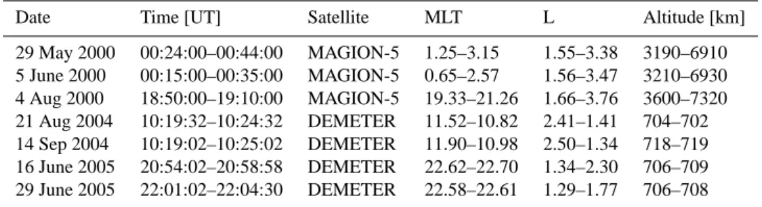
Table 1. Analysed time intervals and selected orbital parameters during the analysed periods.
Date Time [UT] Satellite MLT L Altitude [km]
29 May 2000 00:24:00–00:44:00 MAGION-5 1.25–3.15 1.55–3.38 3190–6910 5 June 2000 00:15:00–00:35:00 MAGION-5 0.65–2.57 1.56–3.47 3210–6930 4 Aug 2000 18:50:00–19:10:00 MAGION-5 19.33–21.26 1.66–3.76 3600–7320 21 Aug 2004 10:19:32–10:24:32 DEMETER 11.52–10.82 2.41–1.41 704–702 14 Sep 2004 10:19:02–10:25:02 DEMETER 11.90–10.98 2.50–1.34 718–719 16 June 2005 20:54:02–20:58:58 DEMETER 22.62–22.70 1.34–2.30 706–709 29 June 2005 22:01:02–22:04:30 DEMETER 22.58–22.61 1.29–1.77 706–708
Fig. 3. Occurrence histogram of time differences twi−tlj between
whistler observation (twi) and lightning discharge detection (tlj).
The histogram corresponds to the analysed period from 00:15 UT to 00:35 UT on 5 June 2000 and to the VLF record by MAGION-5 during the nighttime conditions. Asterisks (magenta) correspond to all discharges, circles (blue) to −CG discharges, crosses (red) to +CG discharges and asterisks (green) to IC discharges.
on 14 September 2004. We can see a distinct peak in both occurrence histograms. This means that the satellites mainly receive the whistlers caused by lightning discharges detected by the EUCLID network in both cases. If this was not true, the time differences would be randomly distributed in the matrix and no distinct peak would occur. Obviously, a re-liability of assigning the causative lightning to a whistler in-creases with the amplitude of the peak relative to the aver-age occurrence rate in the histogram. We remind again that the time difference corresponding to the peak comprises both the propagation time and a possible time shift between the clocks. The possibility of the time shift between the clocks is also the reason why we have searched for the peak in the range of negative time differences, which obviously contra-dicts the causality and has no physical meaning.
Knowing the characteristic time difference correspond-ing to the peak tch=(twi−tlj)peak for each orbit, we can
Fig. 4. Occurrence histogram of time differences twi−tlj
be-tween whistler observation (twi) and lightning discharge
detec-tion (tlj). The histogram corresponds to the analysed period from
10:19:02 UT to 10:25:02 UT on 14 September 2004 and to the VLF record by DEMETER. The meaning of symbols and colours is the same as in Fig. 3.
select only those lightning discharges for which we have found, with great probability, a corresponding whistler in the spectrogram. Once we have found the corresponding pairs “causative lightning-whistler”, we can find the distance be-tween the magnetic footprint of the satellite and the location of the lightning discharge at the given time. Thus, we can in-vestigate the size of the area in the ionosphere trough where the waves enter the magnetosphere. We have analysed data from four orbits of the DEMETER satellite (two of them dur-ing late evendur-ing and two of them durdur-ing the daytime condi-tions) and from three orbits of the MAGION-5 satellite dur-ing the nighttime or evendur-ing conditions. Table 1 summarizes the dates, times, magnetic local times (MLT), L-shell and al-titudes of the satellite during the relevant parts of these orbits. Table 2 gives an overview of the overall number of detected lightning discharges and whistlers. We should note that apart from the fact that the EUCLID network is rather insensitive to IC discharges, the number of detected lightning strokes
2926 J. Chum et al.: Assigning the causative lightning to the whistlers observed on satellites
Table 2. Number of detected lightning discharges and whistlers during the analysed time intervals.
Date Time [UT] Satellite Number of detected Whistlers Number of detected Lightning
29 May 2000 00:24:00–00:44:00 MAGION-5 299 751 5 June 2000 00:15:00–00:35:00 MAGION-5 1722 4093 4 Aug 2000 18:50:00–19:10:00 MAGION-5 185 292 21 Aug 2004 10:19:32–10:24:32 DEMETER 206 499 14 Sep 2004 10:19:02–10:25:02 DEMETER 512 558 16 June 2005 20:54:02–20:58:58 DEMETER 391 137 29 June 2005 22:01:02–22:04:30 DEMETER 259 573
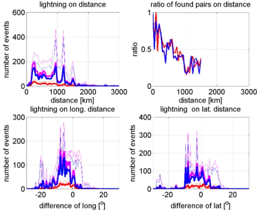
Fig. 5. Distances between the magnetic footprint of the satellite (at the altitude 110 km) and the lightning discharges. Circles (black) are used for all lightning, asterisks (magenta) for those discharges for which the corresponding whistler was found. Positive value of the difference in latitudes (longitudes) means that the footprint was northward (eastward) from the discharge.
also depends on the location of discharges with respect to the sensors (coverage of the network). The number of detected whistlers partially depends on the subjective assessment. We can see that, in our cases, the number of detected lightning strokes is usually larger than the number of whistlers, with the exception of the case on 16 June 2005, when the number of whistlers is larger than the number of lightning discharges. On that day, most of the lightning activity occurred at the bor-der of the area covered by the EUCLID network and hence in an area of a low detection efficiency.
In order to minimize the unwanted influence of the con-figuration “lightning activity – satellite orbit” on our results, we have superposed the results from all the analysed orbits for the time intervals presented in Table 1. The results of the analysis are displayed in Figs. 5 and 6.
Figure 5 shows the distances between the magnetic foot-prints of the satellites and the lightning discharges in the geographic latitude–longitude coordinates. Circles (black) represent all lightning discharges detected by the EUCLID network during the analysed time intervals, whereas aster-isks (magenta) stand only for those discharges for which we have found the corresponding whistler. Figure 6 redis-plays the results presented in Fig. 5 in a form more useful for the interpretation of the results. Different colours distin-guish different types of lightning discharges. Thin lines stand for all detected discharges, whereas thick lines are used only for the discharges for which we have found a corresponding whistler. We present the occurrence histograms of lightning, and the ratios of lightning for which a whistler was found, to all lightning, as a function of the distance between light-ning discharges and magnetic footprints of satellites. We should point out that the values of these ratios are statisti-cally insignificant at distances larger than ∼1500 km – see the number of events in the top left plot. The absolute dis-tances (in km) between the magnetic footprints of the satel-lites and lightning discharges were computed from the given latitudes and longitudes as distances on a spherical model of the Earth’s surface.
We can see that the electromagnetic energy induced by a lightning discharge can enter into the magnetosphere as whistler mode waves at distances up to ∼1500 km (occasion-ally even more) from the discharge. Thus, if the penetrating area is symmetric around the lightning position, its width is two times that distance, which is ∼3000 km. If the situation is asymmetric, the size of the area is less than twice that dis-tance. The decomposition of the distances into longitudinal and latitudinal differences may indicate a certain asymmetry, which can be, however, specific to our data set. The sym-metry/asymmetry of the penetrating area will be discussed in the next section.
The top right plot in Fig. 6 also demonstrates that pos-itive and negative lightning discharges have approximately the same efficiency in producing whistlers, since the curves presenting the ratios of discharges for which whistlers have been found, to all detected discharges, are about same for both +CG and −CG discharges. We cannot say anything
Fig. 6. Top left plot: occurrence histograms of lightning discharges on distance from the magnetic footprints of the satellites. Thick lines stand for the lightning for which the corresponding whistler was found, thin lines stand for all detected lightning. Magenta lines represent all types of discharges, blue −CG discharges, red +CG discharges.
Top right plot: the ratio of lightning discharges for which the corresponding whistler was found to all discharges. Colours distinguish different types of discharges and their meaning is the same as in the top left plot. Note that the values for distances larger than ∼1500 km are statistically insignificant – see the top left plot.
Bottom: Occurrence histogram of the distances between the magnetic footprints of the satellites and lightning discharges decomposed on longitude (left) and latitude (right). The meaning of lines and colours is the same as in the top right plot. The meaning of signs is the same as in Fig. 5.
about the IC discharges, since the EUCLID network is rather insensitive to them; the results related to IC discharges have no statistical significance and are not displayed.
4 Discussion, constraints of the analysis, future work
The plots presented in Figs. 5 and 6 indicate that the lightning-induced waves tend to penetrate the ionosphere in the south-west direction from the lightning discharge. Never-theless, we think that this result might be influenced by spe-cial configurations “lightning activity – satellite orbit” and that more data has to be analysed before we could confirm this result. In our results, the positive values of differences are mostly covered by whistler measurements by MAGION-5 satellite at relatively high L-shells and high altitudes. We should also note that the size of the penetrating area may be slightly overestimated if the propagation of whistlers is nonducted. Thus, future studies should mainly be based on
data from DEMETER or another Low Earth Orbit satellite to be sure that propagation effects do not play any important role. Nevertheless, we should remark that we have not found any remarkable difference between the size of the penetrat-ing area when we analysed cases for DEMETER and MA-GION 5 satellites individually (not shown).
In the present study, we have manually detected several thousand whistlers. An analysis of more data requires us-age of an automatic or quasi-automatic whistler detection. We note that the time resolution of ∼0.1 s, which has the neuronal network instrument “RNF” detecting automatically whistlers on board the DEMETER satellite, is insufficient for this purpose. A reliable automatic detection of fractional-hop whistlers with sufficient time resolution could help us to an-swer the question of whether there is an asymmetry in the area through which the lightning energy enters the magneto-sphere. The software for automatic whistler detection could also enrich the data by the information about the whistler in-tensity.
2928 J. Chum et al.: Assigning the causative lightning to the whistlers observed on satellites We have analysed both daytime and nighttime cases (see
Tables 1 and 2). The results that we obtained for the sepa-rated daytime and nighttime cases did not show remarkable differences (not shown). Again, in order to decide whether there is a difference between the size of the area through which the waves enter the magnetosphere during the night-time and daynight-time conditions, we should analyse more cases, which requires automatic or quasi-automatic whistler detec-tion.
Despite the constraints of our work, we note that the esti-mated size (at least 2000 km) of the area through which the waves enter the magnetosphere is consistent with the size used in numerical simulations of MR whistlers (Shklyar et al., 2004), to obtain the best agreement with the observations of MR whistlers.
5 Conclusions
We have shown that by using a statistical approach it is pos-sible to assign the causative lightning discharges to the ob-served whistlers both on the Low Earth Orbit (LEO) satel-lites, and to the whistlers observed at satellites orbiting at altitudes of ∼5000 km. The assignment is possible both in the nighttime and daytime conditions.
The area in the ionosphere through which the lightning en-ergy leaks into the magnetosphere, and transforms to whistler mode waves is more than 2000 km wide.
We have not observed a higher effectiveness of any type of lightning discharge in producing whistlers. We remark that the EUCLID network is rather insensitive to the IC lightning discharges, therefore the results obtained for these types of discharges are statistically insignificant.
Acknowledgements. The authors would like to acknowledge
J. J. Berthelier for ICE data, and the support by the grant IN-TAS 03-51-4132 and by the grants 205/06/1267 and 205/06/0875 of the grant agency of the Czech Republic. Lightning data were provided by the group of national EUCLID cooperation partners (http://www.euclid.org). The authors also thank both referees for their valuable comments.
Topical Editor M. Pinnock thanks D. Shklyar and another ref-eree for their help in evaluating this paper.
References
Abel, B. and Thorne, R. M.: Electron scattering loss in Earth’s in-ner magnetosphere1. Dominant physical processes, J. Geophys. Res., 103, 2385–2395, 1998a.
Abel, B. and Thorne, R. M.: Electron scattering loss in Earth’s inner magnetosphere 2. Sensitivity to model parameters, J. Geophys. Res., 103, 2385–2395, 1998b.
Barkhausen, H.: Zwei mit Hilfe der neuen Verst¨arker entdeckte Er-scheinungen, Physik A., 20, 401–403, 1919.
Barkhausen, H.: Whistling tones from the Earth, Proc. Inst. Radio Eng., 18, 1155–1159, 1930.
Bell, T. F. and Ngo, H. D.: Electrostatic lower hybrid waves excited by electromagnetic whistler mode waves scattering from planar magnetic field aligned plasma density irregularities, J. Geophys. Res., 95, 149–172, 1990.
Berthelier, J., Godefroy, M., Leblanc, F., Malingre, M., Menvielle, M., Lagoutte, D., Brochot, J., Colin, F., Elie, F., Legendre, C., Zamora, P., Benoist, D., Chapuis, Y., Artru, J., and Pfaff, R.: ICE, the electric field experiment on DEMETER., Planet. Space Sci., 54, 456–471, doi:10.1016/j.pss.2005.10.016, 2006. Bortnik, J., Inan, U. S., and Bell, T. F.: Energy distribution and
life-time of magnetospherically reflecting whistlers in the plasmas-phere, J. Geophys. Res., 108, 1199, doi:10.1029/2002JA09316, 2003.
Brinca, A. L.: On the stability of Obliquely Propagating Whistlers, J. Geophys. Res., 77, 3495–3507, 1972.
Cummins, K. L., Murphy, M. J., Bardo, E. A., Hiscox, W. L., Pyle, R. B., and Pifer, A. E.: A combined TOA/MDF technology up-grade of the U.S. National Lightning Detection Network, J. Geo-phys. Res., 103, 9035–9044, 1998.
Eckersley, T. L.: Musical Atmospherics, Nature, 135, 104–106, 1935.
Gurnett, D. A. and Shawhan, S. D.: Ion Cyclotron Whistlers, J. Geophys. Res., 70, 1665–1688, 1965.
Hayakawa, M., Ohta, K., and Baba, K.: Wave characteristics of tweek atmospherics deduced from the direction-finding measure-ment and theoretical interpretation, J. Geophys. Res., 99, 10 733– 10 743, 1994.
Helliwell, R. A.: Whistlers and Related Ionospheric Phenomena, Stanford University Press, 1965.
Hughes, A. R .W.: Satellite measurements of whistler dispersion at low latitudes, Adv. Space Res., 1, 377–380, 1981.
Hughes, A. R. W. and Rice, W. K.: A satellite study of low latitude electron and proton whistlers, J. Atmos. Solar-Terr. Phys., 59, 1217–1222, 1997.
Imhof, W. L., Voss, H. D., Walt, M., Gaines, E. E., and Mobilia, J.: Slot region electron precipitation by lightning, VLF chorus, and plasmaspheric hiss, J. Geophys. Res., 91, 8883–8894, 1986. Iwai, A., Okada, T., and Hayakawa, M.: Rocket measurement of
wave normal directions of low-latitude sunset whistlers, J. Geo-phys. Res., 79, 3870–3873, 1974.
James, H. G.: Refraction of whistler-mode waves by large-scale gradients in the middle-latitude Ionosphere, Ann. Geophys., 28, 301–339, 1972,
http://www.ann-geophys.net/28/301/1972/.
Kennel, C. F. and Petschek, H. E.: Limit on stably trapped particle fluxes, J. Geophys. Res., 71, 1–28, 1966.
Kimura, I.: Effects of ions on whistler-mode ray tracing, Radio Sci., 1, 269–283, 1966.
Lauben, D. S., Inan, U. S., and Bell, T. F.: Precipitation of radi-ation belt electrons induced by obliquely propagating lightning-generated whistlers, J. Geophys. Res., 106, 29 745–29 770, 2001. Lyons, L. R. and Williams, D. J.: The quiet time structure of ener-getic (35–560 keV) radiation belt electrons, J. Geophys. Res., 80, 943–950, 1975.
Manoranjan, R., Somayajulu, V. V., Dikshit, S. K., and Tantry, B. A. P.: Low-latitude cutoff for whistlers observed on the ground, J. Geophys. Res., 79, 3867–3869, 1974.
Rodger, C. J., Clilverd, M. A., and McCormick, R. J.: Significance of lightning-generated whistlers to inner
tion belt electron lifetimes, J. Geophys. Res., 108, 1462, doi:10.1029/2003JA009906, 2003.
Rycroft, M. J., Israelsson, S., and Price, C.: The global atmo-spheric electric circuit, solar activity and climate change, J. At-mos. Solar-Terr. Phys., 62, 1563–1567, 2000.
Smith, R. L. and Angerami, J. J.: Magnetospheric properties deduced from OGO 1 observations of ducted and nonducted whistlers, J. Geophys. Res., 73, 1–20, 1968.
Shklyar, D., Chum, J., and Jiricek, F.: Characteristic properties of Nu whistlers as inferred from observations and numerical mod-elling, Ann. Geophys., 22, 3589–3606, 2004,
http://www.ann-geophys.net/22/3589/2004/.
Storey, L. R. O.: An investigation of whistling atmospherics, Phil. Trans. Roy. Soc. London, 246, 113–141, 1953.
Yamashita, M.: Propagation of tweek atmospherics, J. Atmos. Terr. Phys., 40, 151–156, 1978.