HAL Id: hal-00330115
https://hal.archives-ouvertes.fr/hal-00330115
Submitted on 1 Feb 2007
HAL is a multi-disciplinary open access
archive for the deposit and dissemination of
sci-entific research documents, whether they are
pub-lished or not. The documents may come from
teaching and research institutions in France or
abroad, or from public or private research centers.
L’archive ouverte pluridisciplinaire HAL, est
destinée au dépôt et à la diffusion de documents
scientifiques de niveau recherche, publiés ou non,
émanant des établissements d’enseignement et de
recherche français ou étrangers, des laboratoires
publics ou privés.
Kelvin-Helmholtz instability
R. Smets, G. Belmont, Dominique Delcourt, L. Rezeau
To cite this version:
R. Smets, G. Belmont, Dominique Delcourt, L. Rezeau. Diffusion at the Earth magnetopause:
en-hancement by Kelvin-Helmholtz instability. Annales Geophysicae, European Geosciences Union, 2007,
25 (1), pp.271-282. �hal-00330115�
www.ann-geophys.net/25/271/2007/ © European Geosciences Union 2007
Annales
Geophysicae
Diffusion at the Earth magnetopause: enhancement by
Kelvin-Helmholtz instability
R. Smets1, G. Belmont1, D. Delcourt2, and L. Rezeau1
1CETP/CNRS/UVSQ/UPMC/IPSL, 10–12 Avenue de l’Europe, 78140 V´elizy, France
2CETP/CNRS/UVSQ/UPMC/IPSL, 4 Avenue de Neptune, 94107 Saint Maur des Foss´es, France
Received: 18 April 2006 – Revised: 18 December 2006 – Accepted: 22 January 2007 – Published: 1 February 2007
Abstract. Using hybrid simulations, we examine how
par-ticles can diffuse across the Earth’s magnetopause because of finite Larmor radius effects. We focus on tangential dis-continuities and consider a reversal of the magnetic field that closely models the magnetopause under southward interplan-etary magnetic field. When the Larmor radius is on the or-der of the field reversal thickness, we show that particles can cross the discontinuity. We also show that with a re-alistic initial shear flow, a Kelvin-Helmholtz instability de-velops that increases the efficiency of the crossing process. We investigate the distribution functions of the transmitted ions and demonstrate that they are structured according to a D-shape. It accordingly appears that magnetic reconnec-tion at the magnetopause is not the only process that leads to such specific distribution functions. A simple analytical model that describes the built-up of these functions is pro-posed.
Keywords. Magnetospheric physics (Magnetopause, cusp, and boundary layers; Magnetosheath; Solar wind-magnetosphere interactions)
1 Introduction
Since the open magnetosphere concept has been proposed by Dungey (1961), possible mechanisms to ensure mass load-ing of the magnetosphere from the shocked solar wind are highly debated. Magnetic reconnection plays a central role in this paradigm to explain the in situ observed coupling be-tween magnetosphere and solar wind. The exact way mag-netic reconnection develops is still controversial, the main reason being that large (MHD) scales have to be coupled with small (electron) scales, which is hardly achieved in
numeri-Correspondence to: R. Smets
cal studies (a same kind of problem occurs in turbulence, see e.g. Frisch, 1995).
Magnetized plasmas consist of particles gyrating around convecting magnetic field lines. When magnetic reconnec-tion occurs, plasma travels in the newly connected regions that were prohibited prior to reconnection. An alternative way to transfer matter across a magnetic boundary is diffu-sion. The topology of the magnetic field lines is preserved, but because of diffusion, particles can jump from one mag-netic field line to another. Because of the collisionless na-ture of the plasma, the origin of diffusion cannot be classi-cal viscosity, and many studies (see e.g. Winske et al., 1995; Treumann et al., 1995) have been dedicated to diffusion pro-cesses in collisionless plasma. On the whole it is commonly admitted that diffusion is less efficient than magnetic recon-nection to ensure mass loading of the inner magnetosphere from the shocked solar wind (see Phan et al., 2005).
The physical process at work at the magnetopause is re-lated to the nature of the magnetic discontinuity: in a tangen-tial discontinuity there is no connection between upstream and downstream plasmas. In contrast, in a rotational discon-tinuity, a normal component of the magnetic field exists that connects both sides. Although the theoretical distinction is clear, experimental evidences are far more complicated be-cause the measurement of a small component of the field is technically difficult. This difficulty is not due to the instru-ments, but to the uncertainty in determining the normal, the planarity of the discontinuity, ... Tests have been developed to check the Rankine-Hugoniot relations and demonstrated that the magnetopause sometimes is a rotational discontinu-ity (Paschmann et al., 1979). In other instances, the mag-netopause is assumed to be a tangential discontinuity (Papa-mastorakis et al., 1984). Recent observations with Cluster (Paschmann et al., 2005) lead to the first statistical studies on the nature of the discontinuity with precise multipoint obser-vations, showing that on the same day both situations can be observed.
Using hybrid simulations, we show that finite Larmor ra-dius (FLR) effects are responsible for anomalous diffusion, due to the thickness of the magnetopause (MP), on the order of the ion Larmor radius (see e.g. Eastmann et al., 1996). Furthermore, at the Earth MP, the shear velocity between the solar wind flowing in the anti-solar direction and the quasi stagnant plasma of the inner magnetosphere can trigger the Kelvin-Helmholtz instability (KHI). The development of such KHI can amplify the diffusion process. The kinetic properties of the plasma are investigated, and compared to the classical structures observed during magnetic reconnec-tion.
In the case of a neutral fluid, Chandrasekhar (1961) showed that KHI develops, regardless of the shear veloc-ity magnitude. Talwar (1964) showed that when there is a component of the magnetic field tangential to the flow, the stabilizing effect of the magnetic tension results in a thresh-old for the instability development. The threshthresh-old as well as the growth rate of the instability is modified by the plasma compressibility (see, e.g. Miura and Pritchett, 1982; Pu and Kivelson, 1983).
Using compressible 2-D MHD code, Miura (1984) showed that up to 2% of the energy flux can cross the magnetic boundary. Miura (1987) also showed that the anomalous tan-gential stress associated with the instability ensures a mo-mentum transport across the discontinuity that can reach a few percents. Still in the MHD interpretation framework, development of KHI can lead to plasma blobs (a direct con-sequence of mass transport, but not the only one) because of resistivity (Nykiri and Otto, 2001), electron inertial ef-fects (Nakamura et al., 2004), or finite Larmor radius efef-fects Huba (1996). KHI may also trigger turbulence (Matsumoto and Hoshino, 2004), and vice-versa, Shinohara et al. (2001) showed that kinetic instability (namely the low hybrid drift instability and the current sheet kink instability) can cascade in KHI.
Using 2-D hybrid simulations, Terasawa et al. (1992) stud-ied the time evolution of a mixing index, providing insights on the total surface close to the instability where particles, initially from both sides of the discontinuity, are mixed. Thomas and Winske (1993) also used 2-D hybrid simula-tions to demonstrate the existence of small-scale structures (on the order of the ion Larmor radius) possibly related to such flux transfer events (see e.g. Southwood et al., 1988, for flux transfer observations). Fujimoto et al. (1994) extended this investigation and focused on mass transport, showing that mixing is quicker and larger than that due to finite Lar-mor radius overlapping at the interface. Thomas (1995) ob-tained similar results with 3-D hybrid simulations for the same geometry, but showed that a rotation of the magnetic field stabilizes the system, and leads to a less efficient mass transport.
Recently, clear observations of the KHI have been reported by Hasegawa et al. (2004) using the four spacecrafts of the Cluster 2 mission. Furthermore, this paper provided
evi-dences of plasma penetration from the magnetosheath into the inner magnetosphere. Interestingly, this paper quotes: “... we could rule out local reconnection because... we did not find signatures of plasma acceleration due to mag-netic stresses and D-shaped ion distribution characteristic of reconnection”. Conversely, one may wonder whether D-shaped distribution functions provide unambiguous signa-tures of magnetic reconnection. We show in this paper that such distribution can actually be observed in the vicinity of a KHI.
In this paper, we will not study in details the develop-ment of the KHI, that is, the possible stabilization by Lan-dau damping as demonstrated by Ganguli (1997), the vor-tex pairing or inverse cascad as put forward by Belmont and Chanteur (1989), or the coupling with smaller scales process (see e.g. Shinohara et al., 2001; Matsumoto and Hoshino, 2004). We use hybrid simulations of the KHI to study the mass transport across the magnetic boundary. Electrons be-ing considered as a massless fluid, we do not resolve electron frequencies. Instabilities like Electron-Ion-Hybrid instability (see Ganguli, 1997; Romero and Ganguli, 1993, 1994) can then not be addressed. In Sect. 2, we describe the hypothe-ses inherent to hybrid simulations. In Sect. 3, we present the model of the initial tangential discontinuity. In Sect. 4, we discuss the development of the KHI. In Sect. 5, we examine the structure of the ion distribution function, and discuss the possible occurence of reconnection. In Sect. 6, we focus on particle dynamics to understand the origin of D-shaped ion distribution functions. In Sect. 7, we exhibit the microscopic process and the implications for spacecraft observations.
2 Simulation model
The calculations are carried out using a hybrid code (ions treated as particles and a massless electron fluid) with two spatial dimensions and three velocity dimensions. Details of the simulation algorithm are given by Winske and Quest (1986). Distances are normalized to the ion inertial length (c/ωP i), time is normalized to the inverse of the ion
gyrofre-quency (ω−1Ci), mass is normalized to the ion mass, and den-sity and magnetic field are normalized to their asymptotic values (the same on each side of the discontinuity), n0 and
B0 , respectively. The size of the simulation box is Xm in
the x-direction and Ym in the y-direction. We use nx=256
grid points in the x-direction, and ny=128 grid points in
the y-direction, Xm=80 and Ym=40 (size of the box in
x-and y-direction), 100 macroparticles per cell x-and a time step 1t =0.005.
In the calculation of the electric and magnetic field, we neglected the displacement curent in the Maxwell-Faraday equation. Such an assumption prevents the development of high frequency modes. Ohm’s law is then needed to define the electric field. Taking into acccount the Hall term, the
electron pressure term and a resistivity, we have
E = −Vi× B +qn1 (J × B − ∇Pe) + ηJ (1)
where Vi is the ion fluid velocity, J the current density, Pe
the scalar electron pressure, η the resistivity, and ne=ni is
the electron (ion) density (noted n hereinafter). We also need a closure equation for the electron fluid. As the development of the KHI is a low frequency process, we used an isothermal equation Pe=nekBTe with a constant value of the electron
temperature Te, kBbeing the Boltzman constant.
We used a small resistivity in these calculations, mainly because of its stabilizing effect on the results, and chose η=0.0001. With this value, the diffusion time is τD=40 000.
The Alfv´en time τA being 2, the growth time of the
resis-tive tearing mode is τr=√2τDτA=400. We will see in the
next section that the simulations are all performed over a to-tal time T =400. Furthermore, KHI starts its linear growth phase at t∼100, and the penetration process starts at the very begining of the simulations. We can thus suspect that there is no magnetic reconnection due to anomalous resistivity that leads to the observed structures. This point will be detailed in Sect. 5 where we discuss the Wal`en test.
The last classical hypothesis concern the boundary condi-tions. Because of the nature of the initial topology, we chose periodic conditions in the x-direction. This assumption can-not be made in the y-direction, because of the reversal of the magnetic field direction, and the bulk flow velocity. At Y =0 and Y =Ym, we assumed that particles are specularly
reflected, and EX=EZ=dYEY=0.
3 Initial topology
We focused on tangential discontinuities with a 180◦rotation angle for the magnetic field. There is thus no normal compo-nent of velocity and magnetic field, and the only constraints for the tangential components are to satisfy the pressure bal-ance. Such a geometry corresponds to the flanks of the MP when the interplanetary magnetic field (IMF) is southward. By definition, the rotation of the magnetic field is in a plane tangential to the discontinuity which we refer to as the XZ plane. As illustrated in Fig. 1, the magnetic field is in the +Z direction in side 1 of the discontinuity, and in the −Z direc-tion in side 2. At the discontinuity, the rotadirec-tion is such that the magnetic field is in the +X direction. The velocity pro-file is also represented, varying from −V0in side 1 to +V0in
side 2.
We use a fluid equilibrium and consider the following pro-file
P0(y) = P1+ (P2− P1)χ (2)
(with 8=(y − Y0)/λ, Y0=Ym/2, and χ =(1+ tanh 8)/2) for
the magnetic field magnitude B0(y), the density n0(y), and
the βi(y) and βe(y) parameter (β being the ratio between
Fig. 1. Schematic view of initial magnetic field and velocity used
in the simulations.
kinetic to magnetic pressure for ions and electrons, respec-tively). The tangential magnetic field is analytically de-scribed by
Bx= B0sin(α) (3)
Bz= B0cos(α) (4)
with α=π(1−χ). We first perform a reference run where the magnetic field magnitude, density, βi and βeparameters
are unifom. We have V0=−V1=V2=0.5, B0=1.0, λ=1.0,
n0=1.0, βi=1.0 and βe=1.0. One remarks there is a gradient
on the magnetic field direction, but not on its magnitude. As discussed later, ions are hence also magnetized in the field reversal region. Except when indicated, these values will also be used in the subsequent runs.
We did not consider any kinetic equilibrium because none of them are satisfactory in our case. Some provided an an-alytical solution for tangential discontinuities with no veloc-ity shear and no magnetic shear (Channell, 1976; Mottez, 2003). Lee and Kan (1979) provided a semi-analytical so-lution of tangential discontinuities including a velocity shear and a small magnetic shear. Roth and DeKeyser (1996) de-scribed a large (though incomplete) class of solutions given as convolution between exponential and error functions. The common problem of these equilibriums is that the proposed solution may not be unique. The numerical equilibrium it-self requires some time (even short) to adjust, either because of numerical uncertainties (inherent to semi-analytical solu-tions), or because the given equilibrium is not the most likely. This adjustment time is inherent to the problem and cannot be avoided. As a result, we used a fluid equilibrium and mon-itored the ion distribution functions to ensure that the equilib-rium is reached before physical processes of interest occur.
To monitor the time evolution of the distribution function at the beginning of the simulation, we rebuilt the 10 indepen-dent components of the heat flux Q. We focus on the heat flux Q because fine structures play an increasing role in the
Fig. 2. Time evolution of the XXY component of the heat flux Q.
high order moments of the distribution functions. The inte-grale to build Q is made on the cells located at Y =Y0,
cor-responding to an integral conducted along the x-direction, at the center of the discontinuity. Being at the center of the dis-continuity, the distribution function strongly depends upon the kinetic equilibrium.
Figure 2 depicts the time evolution of the XXY compo-nent of the heat flux Q. This compocompo-nent of the heat flux is the only one that oscillates at the begining of the simulation, the others being approximately constant. The QXXY value
oscillates with a period about 6, that is close to the gyrope-riod (2π ). After about 3 gyropegyrope-riods, the value of QXXY is
close to zero. Though not represented here, this level is con-stant until T =400. Calculating the QXXY value at different
Y positions, the level of these oscillations proves to be always lower, and reaches the noise level with the same caracteris-tic time. This suggests that a kinecaracteris-tic equilibrium is reached at t ∼20. As we will see hereinafter, the linear growth phase of the KHI starts at t ∼100. Hence, there is no overlapping between the phase during which the equilibrium is reached, and the begining of the KHI development.
Another requirement of this study is to identify the posi-tion of the boundary between side 1 and side 2, at whatever stage of the simulation. To do so, Nykiri and Otto (2001) calculated the z-component of the magnetic vector potential. In the present case, because of the rotation of the magnetic field, a simple definition can be used: we define the MP loca-tion as the localoca-tion where the z-component of the magnetic field changes sign. Figure 3 depicts the z-component of the magnetic field at (a) t=120 (b) t=200 and (c) t=260.
Fig-Fig. 3. Color-coded z-component of the magnetic field at (a) t =120, (b) t =200, and (c) t=260 in the x-y-plane.
ure 3a is the begining of the growing phase of the KHI, where the interface starts to ripple. Figure 3b shows the end of the linear growth phase of the KHI. In this figure, two wave-lengths are noticeable at the interface. During the growing
phase, the wave fronts steepen until saturation. Thereafter, the two waves merge yielding new waves. The number of waves is not very clear in Fig. 3c. Fourier analysis presented later in the paper will help to picture the time evolution. Af-ter t∼260, a new growing phase start, with the build up of 2 new waves fronts that grow until a new saturation. As dis-cussed at the end of Sect. 1, inverse cascad occurence colsely depends on the size of the simulation box.
4 Development of the Kelvin-Helmholtz instability
We start our analysis with the reference run described above. As mentionned in Sect. 3, there is an initial velocity shear and reversal of the magnetic field, with no gradient in density, temperature and magnetic field magnitude. Prior to studying the ion distribution functions, we quantify the effect of the KHI on the mass transport across the discontinuity. We use the δZ value proposed by Thomas and Winske (1993), and defined by
δZ = NT n0Xm
(5) where Xmis the system length in the x-direction, n0the
ini-tial ion density on each side of the boundary, and NT the
total number of ions crossing the interface (from side 2 to side 1) defined in Sect. 3. The crossing process being sy-metric, the NT value computed considering particles
cross-ing from side 1 to side 2 is statistically the same. Even if δZ is homogeneous to a distance, it has to be seen as the normalized number of particles crossing the MP from side 2 to side 1. The time evolution of this quantity is presented in Fig. 4. It should be noted here that at the begining of the sim-ulation, particles close to the boundary may experience re-peated excursions across it. To remove such behaviors from δZ calculated, the value of NT (and thus δZ) is computed
only with particles which remain at least one gyroperiod on the initial side of the discontinuity prior crossing. As a result, one has δZ=0 until t=2π.
In Fig. 4, δZ is strictly growing with time. Between t∼0 and t ∼160, one observes a linear phase during which δZ evolves linearly with time. This demonstrates that the cross-ing process starts at the very begincross-ing of the simulation, when the KHI is not developed yet. Such a behavior was already obtained by Thomas and Winske (1993), and suggests that the crossing process is not directly triggered by the KHI. Be-tween t∼160 and t∼220, a second linear phase is noticeable but with a higher slope value. This interval corresponds to the non-linear stage of the growing phase of the instability. Even though the crossing process is not directly triggered by the KHI, KHI clearly has an influence on this process and en-hances it. Then, we observe a series of phases during which the slope of δZ increases and decreases.
To compare the time evolution of δZ with the stage of the KHI, we calculated the Fourier transform of the spatial se-ries (in the x-direction) of the y-component of the magnetic
Fig. 4. Time evolution of the δZ=NT/n0Xmlayer thickness.
field, averaged in the y-direction. In Fig. 5, we show the log-arithm of this value (color-coded) as a function of time and KXmode. We also calculated the time derivative of δZ. The
obtained value being quite noisy (as usual with numerical derivative calculation), we filtered it with a gaussian window of 8 points width. The obtained result is multiplied by a nor-malization coefficient (to fit the KXscale) and displayed with
solid thick line in Fig. 5. At t ∼100, the KHI develops and grows until t∼200. This can be seen in, Fig. 5 by the broad-ening of the BY spectra. At t∼200, the instability reaches
its saturation level after what, vortex coalescence is observed until t∼250. This phase clearly corresponds to a lowering of the spectral width of BY. We then observe until t =400
two others saturation stages, preceded by a growing phase, and followed by a coalescence phase. One can note a good agreement between the time derivative of δZ and the spectral width of BY.
For the sake of clarity, we introduce the following denom-ination for the particle orbits: we call “short crossings” parti-cles that cross several times the discontinuity, with a time of flight between 2 crossings smaller than 2π , and “long cross-ings” particles that cross the discontinuity several times, with a time of flight between two crossings larger than 2π . We must also make a distinction between even number of cross-ings and odd number of crossing: odd values are associated to particles that change sides, whereas even values are asso-ciated to particles that end up on the same side of the discon-tinuity as they were initially.
Fig. 5. Color-coded Y component of the magnetic field depending
on the Kx mode (after spatial Fourier transformation) and time. The solid thick line is the time evolution of the derivative of δZ.
5 Ion distribution functions
In this section, we build the ion distribution functions asso-ciated with particles that cross the discontinuity. Building ion distribution functions requires to define a protocol. In-deed, with particle-like simulations, distribution function re-sults from an average on a statistically representative popu-lation. In the same way as in Fig. 4, distribution functions correspond to particles that cross the discontinuity, with an initial time of flight prior to the first crossing at least equal to 2π .
Figure 6 displays the number of crossing particles color-coded in each cell (of size 1X by 1Y ), depending on their X and Y position at t=240. The solid line indicates the position of the MP identified by the sign change of BZ. Figure 6 does
not take into account “short crossing”, but only particles that cross once the discontinuity. Hence, particles on sides 2 were initially on side 1 and vice-versa. One can clearly see that the crossing particles form islands located between the edges of the surface instability. Crossing particles being located in small regions, we build the distribution function associated with these 4 islands (2 on each side).
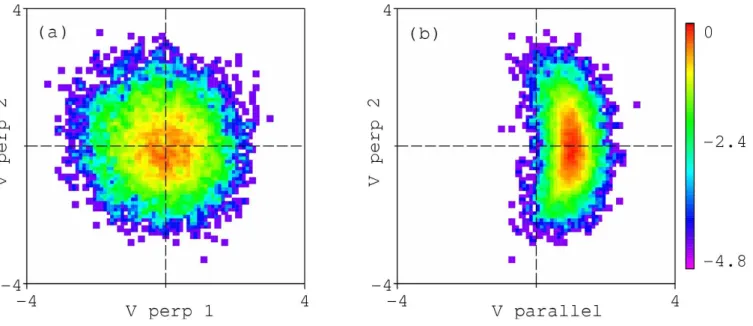
Figure 7 depicts the ion distribution functions at t=240 associated with particles that experience 2 crossings. Since we have very similar distribution functions in these 4 islands (whatever the side we consider), the one presented in Fig. 7 shows an average over all islands. The left and right panel of Fig. 7 show the color coded phase space density in the plane perpendicular to the local magnetic field and in the paral-lel – perpendicular velocity direction, respectively. The left panel of Fig. 7 reveals that the distribution is gyrotropic. This
Fig. 6. Color-coded number of particles crossing once the
disconti-nuity.
result is not unexpected: because of the constraints on the time of flight, the distribution functions correspond to parti-cles that experience an adiabatic motion. The hypothesis of random gyrophases is thus satisfied. Furthermore, the com-puted value of the temperature is approximately the same as the one used for the initialization. No evidence of heating or cooling is noticeable.
In the right panel of Fig. 7, a D-shaped distribution can be seen, most particles having a positive value of their par-allel velocity. One should note that the sign of the bulk flow associated to the D-shaped distribution (positive in Fig. 7) does not depend on the side of the MP where it is observed. As mentioned earlier, the particles considered here fly more than 2π after crossing the discontinuity. If this time of flight is increased the same overall pattern is observed, with just a slightly smaller number of particles. As discussed in the introduction, the build-up of such D-shaped distributions is often associated with magnetic reconnection when such D-shaped distribution is observed (see e.g. Cowley and Shull, 1983). We already saw that the numerical resistivity is sup-posedly too small to let resistive tearing occur. To explore this distribution further and rule out the occurence of mag-netic reconnections, we perform Wal`en test (see e.g. Son-nerup et al., 1981).
This test consists in comparing the fluid velocity to the Alfv´en velocity (for both x- and y-components). To do so, we build at t=240, the components of the Alfv´en and fluid velocity from the magnetic and fluid structures we computed along a virtual crossing, at X=25, and between Y =20.3 and Y =26.5. This arises from the position of the MP, located (at X=25) at Y =23.4 and corresponds to 20 cells (10 in each
Fig. 7. Color-coded phase space density of crossing particles (see text): (left) in the perpeendicular plane (right) in the parallel-perpendicular
plane.
Fig. 8. (Left) normal and (right) tangential fluid velocity as a function of Alfv´en speed.
sides of the MP) that gives 20 couples of Alfv´en and fluid ve-locity (in both x- and y-direction). In Fig. 8, we show the dis-tinct values of these couples (x-component on the left panel and y-component on the right panel) and check whether there exists a possible value of the deHoffmann-Teller frame ve-locity VH T that can verify the test V =VH T±VA.
Figure 8 demonstrates that the Wal`en test is not satisfied because there is no way to interpolate these points with a straight line having a slope equal to one. Similar calculations changing the localization and/or the stage of the KHI lead to the same conclusion. Accordingly, there is no magnetic reconnection in the present set of simulations. Starting from a tangential discontinuity, regardless of the stage of the KHI,
Table 1. Parameters used for different runs. λ is the initial half
thickness of the discontinuity, V0, B0and n0the initial asymptotic
value of the fluid velocity, magnetic field magnitude and density, respectively, and βi the ionic β parameter.
Run parameters set Run 1 reference Run 2 λ=1.1, V0=0.7
Run 3 λ=1.2, B0=1.4
Run 4 λ=1.3, n0=0.6
Run 5 λ=1.4, opposite polarization Run 6 λ=1.6, βi=2.0
Run 7 λ=1.8, βi=2.0, B0=0.7
the discontinuity never becomes rotational. To understand the building of the D-shaped distributions, one must consider the charged particles dynamics.
6 Particle dynamics
With the D-shaped distribution obtained in Fig. 7, we calcu-late the associated mean parallel velocity noted Vk. A variety of runs were performed to characterize the conditions of oc-curence of such distributions, as well as the computed value Vk. They are summarized in Table 1. As indicated in Sects. 2 and 3, we have for run 1, λ=1.0, V0=0.5, B0=1.0, n0=1,
βi=1.0, βe=1.0. We indicate for the other runs values that
differs from these ones. This choice of parameters allows to explore differents values of the Alfv´en velocity, of the shear velocity, of the thermal Larmor radius, and of the polariza-tion of the discontinuity. For these 7 runs, we construct the ion distribution function as in Fig. 7. They are not depicted here, but in all cases, D-shaped structures are obtained. The efficiency of the penetration process can differ from one run to another by a factor of 2, which has (for our purpose) only consequences on the statistics to calculate Vk.
We performed some other runs reversing the velocity shear direction and/or the direction of the asymptotic magnetic field, and obtained that it does not change the positive value of the mean parallel velocity in the D-shaped ion distribu-tion funcdistribu-tion. The only way to achieve this is to reverse the sense of rotation of the magnetic field of the initial tangential discontinuity (being thus initially in the −X direction at the interface between side 1 and side 2). Other test runs showed that the magnitude of this mean parallel velocity only de-pends on the initial half thickness of the discontinuity λ and on the magnitude of the initial asymptotic magnetic field.
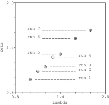
We computed the mean parallel velocity Vkand calculated the ζ value, defined as
ζ = Vk C
(6)
Fig. 9. Computed ζ value as a function of the initial half thickness
λ.
where C is the gyroperiod with the asymptotic magnetic
field magnitude. This is the average distance traveled along the magnetic field by the particle (forming the core of the D-shaped ion distribution function) during a cyclotron turn.
Figure 9 depicts the computed ζ value, depending on the initial λ value. It can be seen in this figure that a straight line with a slope close to one connects the various runs. Accord-ingly, the building of a D-shaped structure does not depend upon the magnitude of the Alfv´en velocity or the shear ve-locity. We thus suspect the magnetic field rotation to play a role in this process. This idea is strenghtened by the fact that reversing the sense of rotation of the magnetic field changes the sign of the mean parallel velocity associated to distribu-tion funcdistribu-tion. To examine this issue further, we examined test particle orbits.
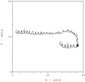
Figure 10 shows the orbit of a particle in the time vary-ing electric and magnetic field durvary-ing T =200. This particle starts initially at X∼4 and Y ∼22 on side 2. Following the shear velocity, this particle drifts in the +X direction. White triangles are drawn every 1T =20. Around t=160, the parti-cle crosses the discontinuity (indicated by the black triangle), and ends up on side 1 of the discontinuity until the end of the simulation. This type of orbit is representative of particles that compose the bulk of the D-shaped structure. In other words, these particles never exhibits short crossing, and sel-dom long crossing. Crossing always occurs on time scale on the order of the gyroperiod, with nearly-adiabatic sequences prior to and after this crossing. One can understand that, in view of Fig. 10, the structure of the magnetic field, even if corrugated through time, has a structure in the z-direction similar to the field reversal initially imposed.
Fig. 10. Orbit of a crossing particle calculated self-consistently.
Such behaviors were already reported in Smets (2000). They are not due to the curvature of the magnetic field lines (the initial magnetic field lines being straight lines as indi-cated in Fig. 1), but to the scale of the field reversal. In a like manner to the adiabatic parameter κBZ defined by B¨uchner
and Zelenyi (1989), Smets (2000) defined the κRSparameter
(RS standing for Reversal Sheet) as the square root of the ra-tio between the thickness of the reversal sheet and the maxi-mum Larmor radius. This study is hence done at κRS∼1, and
as predicted by Smets (2000), we never observe Speiser-like orbits and particle trapping at the interface, because of FLR effects. This type of non-linear dynamics has been reported by Smets (2002) using test-particle calculations in realistic magnetic topologies, obtained by MHD simulation of the KHI. But this work was done at κRS∼0.6 which, as
demon-strated by Smets (2000), allows particle trapping.
As we already saw in Fig. 4, penetration process starts at the begining of the simulation, before the KHI develops. We can suspect that this process is not directly linked to the oc-curence of the KHI, but rather to the magnetic topology of the discontinuity. The KHI just appears as a speeding up fac-tor for the penetration process.
7 Microscopic process
A heuristic interpretation of the penetration process can be obtained with a rough picture of the magnetic field reversal. As a matter of fact, details of the magnetic profile (hyperbolic tangent in the present case) is not necessary and knowledge of the asymptotic value of the magnetic field in each side and
Fig. 11. Schematic view of the typical orbit followed by a particle
crossing the magnetic field reversal.
at the center of the discontinuity is enough to drive the essen-tial features. The associated process is depicted in Fig. 11. We considered side 1 and 2 with a magnetic field that is con-sidered constant, in the +Z direction and −Z direction, re-spectively and we neglect the drift effect of the electric field: the associated fluid velocity being tangential to the disconti-nuity, it does not play a significant role in this process. At the interface, we consider also a constant magnetic field, in the +X direction that we call reversal sheet.
Let us consider a particle, initially on side 2, with a pos-itive parallel velocity. Starting from an initial position with positive Z value, this particle, because of its parallel veloc-ity, goes toward the Z=0 plane. Furthermore, because of the magnetic field and its perpendicular velocity, the particle gy-rates around a magnetic field line, with a constant Larmor radius. With the appropriate initial position (as chosen in Fig. 11), this particle skims the interface between side 2 and the reversal sheet. When at the interface, because of mag-netic noise, the particle can step aside, in the reversal sheet. This point is marked A in Fig. 11, and for simplicity, cho-sen to be in the Z=0 plane. To reach side 1 at point marked B, the Larmor radius in the reversal sheet has to be equal to the half thickness of the discontinuity λ. At point A, the per-pendicular velocity needed in the calculation of the Larmor radius is in the −Z direction, that is the parallel velocity in side 2. Because there is no electric field, the kinetic energy of the particle is constant, and the parallel velocity in side 1 is equal to the parallel velocity in side 2 (that turns to be a perpendicular velocity in the reversal sheet).
The above explanation is based on geometric arguments, and does not depend upon the details of the discontinuity, provided it is tangential. This suggests that the analytical profile that we chose for the magnetic field is not critical. On the other hand, it is clear from Fig. 5 that magnetic field as-sociated to high values of KXplays an important role in this
Fig. 12. Color-coded number of particles crossing the magnetic field reversal. Left panel depicts the final value of the parallel velocity,
depending on its initial value, and right panel depicts the final value of the perpendicular velocity, depending on its initial value.
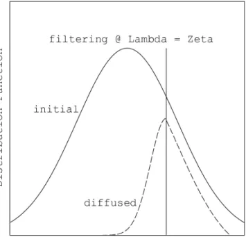
Fig. 13. Schematic view of the filtering effect acting upon the initial
ion distribution function to produce a D-shaped one.
components of the electric field, and did not get any correla-tion between electric noise and enhancement of penetracorrela-tion process. It seems that magnetic noise is the essential source of penetration, even if ruling out the role of the electric noise would require us to perform some other runs with an appro-priate low band filtering.
With the mechanism we just described, we explain easily why the crossing paticles are the one for which the computed ζ value is equal to λ. Further insights into this mechanism may be obtained from Fig. 12 that shows the initial particle velocity depending on its final value. Left panel of Fig. 12 is for parallel velocity, and right panel for perpendicular ve-locity. The first remark is that we have a clear symetry about the first bisector of the axis. In the left panel of Fig. 12, the largest number of particles crossing the interface is for both initial and final parallel velocity close to one, that is con-sistent with the mechanism discussed above. Furthermore, following the isocontour associated to the highest number of crossings, particles with a final parallel velocity larger than one have an initial parallel velocity smaller than one, and vice-versa. This is also consistent with the proposed mecha-nism. Going back to Fig. 11, let us consider a particle reach-ing point A with a parallel velocity givreach-ing a ζ value larger than λ. The Larmor radius in the reversal sheet being larger than λ, the particle will reach side 1 before achieving a com-plete half cyclotron turn. Thus, only a fraction of the perpen-dicular velocity in the reversal sheet will end-up in parallel velocity in side 1. This is the reason why crossing parti-cles with large initial parallel velocity have a smaller one af-ter crossing the discontinuity. This process being totally sy-metric, we explain in the very same way why particles with a small initial parallel velocity will have a larger one after crossing the discontinuity. In these two cases, initial paral-lel (perpendicular) velocity can transform in perpendicular (parallel) velocity after crossing the discontinuity, and vice-versa. This clearly explains the right pattern of Fig. 12.
8 Discussion
The process described here can be viewed as a filter for the crossing particles. Figure 13 shows a schematic view of the distribution function, depending on the parallel veloc-ity. The solid line represents the initial distribution function, the dashed line represents the distribution function associ-ated with the crossing particles. For simplicity, we neglect the mean value of the bulk velocity in the initial distribution function. The vertical line represents the parallel velocity for which we have ζ =λ. Particles with a parallel velocity larger than this value are able to cross the discontinuity. The others can hardly achieve it.
The resulting D-shaped distribution is only associated with crossing particles. At a given point, there is no way to ex-perimentally distinguish between crossing particles and non-crossing particles. This means that the observed distribution results from the superposition of a drifting maxwellian asso-ciated to the non-crossing particles, and a D-shaped distribu-tion associated to crossing particles. Construcdistribu-tion of realistic distribution is beyond the scope of this paper, but calculat-ing the mixcalculat-ing index as suggested by Terasawa et al. (1992), we found that there exists regions where the proportion of crossing/non-crossing particles is half-half (at t=400). We claim that, even if fuzzed, D-shaped distribution should be observable in the vicinity of the MP, when the IMF is south-ward.
The spatial extension of the region in which such D-shaped distribution are observable around a tangential discontinuity is questionable. From Fig. 6, it appears that it is around the field reversal on a layer thickness of about 20 (even if it is not filled only by crossing particles). This layer may actu-ally be much thicker since we have seen that the penetration process depends on the thickness of the discontinuity (only its efficiency depends on the KHI phase), ζ being a linear function of λ. The small value of δZ is clearly due to the fact that δZ=0 at t=0. As long as the thickness of the dis-continuity remains constant (and we have no evidence of its enhancement) we will have penetration process. A proper answer to this question would need an asymptotic study of this behavior, on a time much larger than a few hundreds of ionic cyclotronic periods to reach a stationary state.
There also exists a density gradient at the MP. This gradi-ent can be located at a differgradi-ent location from the magnetic field gradient that defines the boundary layer. We do not con-sider such a density gradient, and will explain why it is not a problem for our results. We computed two runs with a den-sity gradient at the interface, one with a denden-sity ratio equal to 4, and another with a ratio equal to 10 (which is a quite realistic value at the MP, see e.g. Paschmann et al., 1978). We observe the same process of discontinuity traversal, and a D-shaped distribution. The relation between λ and ζ is still linear, but with a different value of the slope (depending on the density gradient). The diamagnetic drift associated with such a density gradient should then be considered in the
ex-planation. But the important point however is that, looking at in situ observations, the density gradient can occur at a differ-ent location from the gradidiffer-ent of the magnetic field direction: density gradient and field reversal can then be decoupled (see e.g. Paschmann et al., 1978). Observations also show a thin-ner MP with a southward IMF than with a northward one, and a density gradient (considered as the MP thickness) thicker than the field reversal layer. The consequences of these re-marks are that calculations with a realistic density gradient should not affect the build-up of D-shaped distribution if the density gradient is not located at the same position as the field reversal. If both density gradients and field reversal oc-cur at the same location, this would only change the relation between λ and ζ , but not the overall structure of a D-shaped distribution.
9 Conclusions
The hybrid simulations performed demonstrate that in a tan-gential discontinuity as is the case in the flanks of the mag-netosphere during southward IMF conditions, the KHI does not trigger the transport of matter across the MP but rather enhances and/or speed up it. The transmitted particles ex-hibit D-shaped distribution, the average parallel speed being controlled by the half thickness of the discontinuity and the asymptotic magnetic field magnitude. We hence conclude that there is no one-to-one relationship between magnetic re-connection and D-shaped distribution functions as is com-monly postulated.
Acknowledgements. Part of this work was done while R. Smets held
a grant from CNRS/JSPS # 12852 for a mid-term stay at University of Tokyo. R. Smets thanks M.. Hoshino, A. Miura, T. Terasawa, and Y. Matsumoto for fruitfull discussions, and M. Hesse for providing the hybrid code.
Topical Editor I. A. Daglis thanks G. Ganguli and another ref-eree for their help in evaluating this paper.
References
Belmont, G. and Chanteur, G.: Advances in magnetopause Kelvin-Helmholtz instability studies, Phys. Scripta, 40, 124–128, 1989. B¨uchner, J. and Zelenyi, L. M.: Regular and chaotic charged
par-ticle motion in magnetotaillike field reversal 1. Basic theory of trapped motion, J. Geophys. Res., 94, 11 821–11 842, 1989. Chandrasekhar, S.: Hydrodynamic and hydromagnetic stability,
Dover Publication, New York, 1961.
Channell, P. J.: Exact Vlasov-Maxwell equilibria with sheared mag-netic fields, Phys. Fluids, 19, 1541–1545, 1976.
Cowley, S. W. H. and Shull Jr., P.: Current sheet acceleration of ions in the geomagnetic tail and the properties of ions bursts observed at the lunar distance, Planet. Space Sci., 31, 235–245, 1983. Dungey, J. W.: Interplanetary magnetic field and the auroral zone,
Eastman T. E., Fuselier, S. A., and Gosling, J. T.: Magnetopause crossing without a boundary layer, J. Geophys. Res., 101, 49–57, 1996.
Frisch, U.: Turbulence, Cambridge University Press, 296 pages, 1995.
Fujimoto, F. and Terasawa, T.: Anomalous ion mixing within and MHD scale Kelvin-Helmholtz vortex, J. Geophys. Res., 99, 8601–8613, 1994.
Ganguli, G.: Stability of an inhomogeneous transverse plasma flow, Phys. PLasmas, 4, 1544–1551, 1997.
Hasegawa, H., Fujimoto, M., Phan, T.-D., R`eme, H., Balogh, A., Dunlop, M. W., Hashimoto, C., and TanDokoro, R.: Transport of solar wind into Earth’s magnetosphere through rolled-up Kelvin-Helmholtz vortices, Nature, 430, 755–758, 2004.
Huba, J. D.: The Kelvin-Helmholtz instability: Finite Larmor ra-dius magnetohydrodynamics, Geophys. Res. Lett., 23, 2907– 2910, 1996.
Lee. L. C. and Kan, J. R.: A unified model of the tangential magne-topause structure, J. Geophys. Res., 84, 6417–6426, 1979. Matsumoto, Y. and Hoshino, M.: Onset of turbulence induced by
a Kelvin-Helmholtz vortex, Geophys. Res. Lett., 31, L028071– L028074, 2004.
Miura, A. and Pritchett, P. L.: Nonlocal stability analysis of the MHD Kelvin-Helmholtz instability in a compressible plasma, J. Geophys. Res., 87, 7431–7444, 1982.
Miura, A.: Anomalous transport by magnetohydrodynamic Kelvin-Helmholtz instabilities in the solar wind-magnetosphere interac-tion, J. Geophys. Res., 89, 801–818, 1984.
Miura, A.: Simulation of the Kelvin-Helmholtz instability at the magnetospheric boundary, J. Geophys. Res., 92, 3195–3206, 1987.
Mottez, F.: Exact nonlinear analytic Vlasov-Maxwell tangential equilibria with arbitrary density and temperature profiles, Phys. Plasmas, 10, 2501–2508, 2003.
Nakamura, T. K. M., Hayashi, D., and Fujimoto, M.: Decay of MHD-scale Kelvin-Helmholtz vortices mediated by parasitic electron dynamics, Phys. Rev. Lett., 92, 145001-1–145001-4, 2004.
Nykiri, K. and Otto, A.: Plasma transport at the magnetospheric boundary due to reconnection in Kelvin-Helmholtz vortices, Geophys. Res. Lett., 28, 3565–3568, 2001.
Papamastorakis, I., Paschmann, G., Sckopke, N., Bame, S. J., and Berchem, J.: The magnetopause as a Tangential discontinuity for large field rotation angles, J. Geophys. Res., 89, 127–135,1984. Paschmann, G., Sckopke, N., Haerendel, G., Papamastorakis, J.,
Bame, S. J., Asbridge, J. R., Gosling, T. J., Hones Jr., E. W., and Tech, E. R.: ISEE plasma observations near the subsolar magnetopause, Space Sci. Rev., 22, 717–737, 1978.
Paschmann, G., Sonnerup, B. U. O., Papamastorakis, I., Sckopke, N., Hearendel, G., Bame, S. J., Asbridge, J. R., Gosling, J. T., Russell, C. T., and Elphic, R. C.: Plasma acceleration at the Earth’s magnetopause: evidence for reconnection, Nature, 282, 243–246, 1979.
Paschmann G., Haaland, S., Sonnerup, B. U. O., Hasegawa, H., Georgescu, E., Klecker, B., Phan, T.-D., R`eme, H., and Vaivads, A.: Characteristics of the near-tail dawn magnetopause and boundary layer, Ann. Geophys., 23, 1481–1497, 2005,
http://www.ann-geophys.net/23/1481/2005/.
Phan, T. D., Escoubet, C. P., Rezeau, L., Treumann, R. A., Vaivads, A., Paschmann, G., Fuselier, S. A., Atti, D., Rogers, B., and Son-nerup, B. U. O.: Magnetopause Processes, Space Sci. Rev., 118, 367–424, 2005.
Pu, Z. Y. and Kivelson, M. G.: Kelvin-Helmholtz instability at the magnetopause: solution for a compressible plasma, J. Geophys. Res., 88, 841–852, 1983.
Romero, H. and Ganguli, G.: Nonlinear evolution of a strongly sheared cross-field plasma flow, Phys. Fluids, 5, 3163–3181, 1993.
Romero, H. and Ganguli, G.: Relaxation of the stressedd plasma sheet boundary layer, Geophys. Res. Lett., 21, 645–648, 1994. Roth, M., DeKeyser, J., and Kuznetsova, M. M.: Vlasov theory of
the equilibrium structrure of tangential discontinuities in space plasmas, Space Sci. Rev., 76, 251–317, 1996.
Shinohara, I., Suzuki, H., Fujimoto, M., and Hoshino, M.: Rapid large-scale magnetic-field dissipation in a collisionless current sheet via coupling between Kelvin-Helmholtz and lower-hybrid drift instabilities, Phys. Rev. Lett., 87, 095001-1–095001-4, 2001.
Smets, R.: Charged particle dynamics in a tangential discontinuity, J. Geophys. Res., 105, 25 009–25 019, 2000.
Smets, R., Delcourt, D., Chanteur, G., and Moore, T. E.: On the incidence of the Kelvin-Helmholtz instability for mass exchange process at the Earth’s magnetopause, Ann. Geophys., 20, 757– 769, 2002,
http://www.ann-geophys.net/20/757/2002/.
Sonnerup, B. U. O., Paschmann, G., Papamastorakis, I., Sckopke, N., Haerendel, G., Bame, S. J., Asbridge, J. R., Gosling, J. T., and Russell, C. T.: Evidence for magnetic field reconnection at the Earth magnetopause, J. Geophys. Res., 86, 10 049–10 067, 1981.
Southwood, D. J., Farrugia, C. J., and Saunders, M. A.: What are Flux Transfer events?, Planet. Space Sci., 36, 503–508, 1988. Talwar, S. P.: Hydromagnetic stability of the magnetospheric
boundary, J. Geophys. Res., 70, 2707–2713, 1964.
Terasawa, T., Fujimoto, M., Karimabadi, H., and Omidi, N.: Anomalous ion mixing within a Kelvin-Helmholtz vortex in a collisionless plasma, Phys. Rev. Lett., 68, 2778–2781, 1992. Thomas, V. A. and Winske, D.: Kinetic simulation of the
Kelvin-Helmholtz instability at the magnetopause, J. Geophys. Res., 98, 11 425–11 438, 1993.
Thomas, V. A.: Three-dimensional kinetic simulation of the Kelvin-Helmholtz instability, J. Geophys. Res., 100, 19 429–19 433, 1995.
Treumann, R. A., LaBelle, J., and Bauer, T. M.: Diffusion pro-cesses: an observational perspective, Geophys. Monograph, 90, 331–341, 1995.
Winske, D. and Quest, K. B.: Electromagnetic ion beam instabil-ities: Comparison of one- and two-dimensional simulations, J. Geophys. Res., 91, 8789–8797, 1986.
Winske, D., Thomas, V. A., and Omidi, N.: Diffusion at the mag-netopause: a theoretical perspective, Geophys. Monograph, 90, 321–329, 1995.