HAL Id: hal-00316220
https://hal.archives-ouvertes.fr/hal-00316220
Submitted on 1 Jan 1996
HAL is a multi-disciplinary open access
archive for the deposit and dissemination of sci-entific research documents, whether they are pub-lished or not. The documents may come from teaching and research institutions in France or abroad, or from public or private research centers.
L’archive ouverte pluridisciplinaire HAL, est destinée au dépôt et à la diffusion de documents scientifiques de niveau recherche, publiés ou non, émanant des établissements d’enseignement et de recherche français ou étrangers, des laboratoires publics ou privés.
On the assimilation of total-ozone satellite data
P. F. Levelt, M. A. Allaart, H. M. Kelder
To cite this version:
P. F. Levelt, M. A. Allaart, H. M. Kelder. On the assimilation of total-ozone satellite data. Annales Geophysicae, European Geosciences Union, 1996, 14 (11), pp.1111-1118. �hal-00316220�
Correspondence to: P. F. Levelt
Ann. Geophysicae 14, 1111—1118 (1996) ( EGS — Springer-Verlag 1996
On the assimilation of total-ozone satellite data
P. F. Levelt, M. A. F. Allaart, H. M. Kelder
Royal Netherlands Meteorological Institute (KNMI), 3730 AE De Bilt, The Netherlands Received: 2 November 1995/Revised: April 1996/Accepted: 3 April 1996
Abstract. A two-dimensional model for advection and data assimilation of total-ozone data has been developed. The Assimilation Model KNMI (AMK) is a global model describing the transport of the column amounts of ozone, by a wind field at a single pressure level, assuming that total ozone behaves as a passive tracer. In this study, ozone column amounts measured by the TIROS Opera-tional Vertical Sounder (TOVS) instrument on the Na-tional Oceanic and Atmospheric Administration (NOAA) polar satellites and wind fields from the Meteorological Archive and Retrieval System (MARS) archives at ECMWF have been used. By means of the AMK, the incomplete space-time distribution of the TOVS measure-ments is filled in and global total-ozone maps at any given time can be obtained. The choice of wind field to be used for transporting column amounts of ozone is extensively discussed. It is shown that the 200-hPa wind field is the optimal single-pressure-level wind field for advecting total ozone. Assimilated ozone fields are the basic in-formation for research on atmospheric chemistry and dynamics, but are also important for the validation of ozone measurements.
1 Introduction
Satellite measurements and ground-based measurements of ozone are essential for understanding the dynamical and chemical behaviour of ozone, for studying the ozone-hole phenomena, for detecting trends in the ozone distri-bution and for determining the climatology of ozone. Global coverage of satellite measurements is important for most of these studies mentioned. Global total-ozone measurements are produced by satellite instruments like the Total Ozone Monitoring Spectrometer (TOMS) (Stolarski et al., 1991), the Solar Backscatter Ultraviolet
Radiometer (SBUV) (Heath et al., 1975), the TIROS Op-erational Vertical Sounder (TOVS) (Planet et al., 1984), the Global Ozone Monitoring Experiment (GOME) (Hahne et al., 1993) and, in the near future, the Scanning Imaging Absorption Spectrometer for Atmospheric Car-tography (SCIAMACHY) on board of ENVISAT (ESA’s, European Space Agency, Environmental Satellite) and the Ozone Monitoring Instrument (OMI) (ESA document, in
preparation, 1996) on board of METOP (EUMETSAT’s,
European Organization for the Exploration of Meteoro-logical Satellites, MeteoroMeteoro-logical Operational Program). The GOME instrument on board of the ERS-2 satellite, ESA’s Earth Resource Satellites, was launched in April 1995. GOME measures ozone and other trace gases and has a swath width of 960 km. This will result a global coverage in three days.
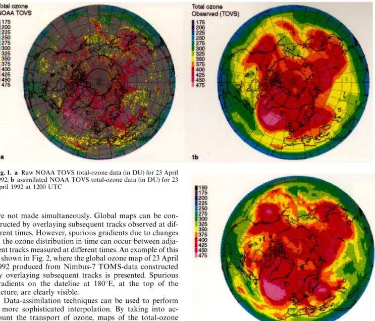
For several of the mentioned studies, monitoring of the distribution of ozone is needed on a daily basis. However, the ozone maps are often hampered by missing data due to, for example, retrieval problems in the case of clouds (TOVS) or limited swath width (SBUV, GOME). In these cases only sparse data are obtained, and it is often difficult to characterise features in the ozone distribution. The atmospheric circulation and the total-ozone content of the atmosphere are strongly correlated. This has already been recognised for the northern hemisphere for almost seventy years (Dobson et al., 1928 and Dobson, 1968). In general, a high-pressure region will give rise to low ozone values, while an extratropical low will show up as a region with high gradients in total-ozone values and high total-ozone values behind the centre of the low (Heijboer et al., 1996). This relation can be quantified using the correlation be-tween vertically integrated potential vorticity and total ozone, as found by Allaart et al. (1993). In Fig. 1a, a map of retrieved TOVS satellite data measured on 23 April 1992 is shown. The data have been gathered over a period of 24 h. Due to missing data (normally only one-third of the globe is covered with TOVS data), it is difficult to recog-nise specific features or coherent structures in the global ozone field. Another fundamental problem with the use of data from polar orbiting satellites is that the observations
Fig. 2. NASA TOMS total-ozone map (in DU) for 23 April 1992. Spurious gradients are visible at the date line 180°E (top of the
picture)
Fig. 1. a Raw NOAA TOVS total-ozone data (in DU) for 23 April 1992; b assimilated NOAA TOVS total-ozone data (in DU) for 23 April 1992 at 1200 UTC
are not made simultaneously. Global maps can be con-structed by overlaying subsequent tracks observed at dif-ferent times. However, spurious gradients due to changes in the ozone distribution in time can occur between adja-cent tracks measured at different times. An example of this is shown in Fig. 2, where the global ozone map of 23 April 1992 produced from Nimbus-7 TOMS-data constructed by overlaying subsequent tracks is presented. Spurious gradients on the dateline at 180°E, at the top of the picture, are clearly visible.
Data-assimilation techniques can be used to perform a more sophisticated interpolation. By taking into ac-count the transport of ozone, maps of the total-ozone distribution at any given time can be produced. For this purpose a two-dimensional (latitude/longitude) advection and data-assimilation model has been developed [the Assimilation Model KNMI (AMK)] in which total ozone is advected by a wind field at a single pressure level. The data assimilation is performed by taking weighted aver-ages of advected ozone and ozone-satellite measurements. To our knowledge this is one of the first times in which a data-assimilation technique has been used for total ozone. The model uses wind fields from the European Centre for Medium Range Weather Forecasts (ECMWF) model and total-ozone data measured by the TOVS in-struments; i.e. AMK is an off-line model which does not calculate its own wind field. The three-dimensionality of the atmosphere versus the two-dimensionality of total ozone poses however a problem. Total-ozone data do not determine in a unique way the ozone profile. If a three-dimensional model is used for the advection, an approach is to assume a vertical ozone distribution, and normalise this with total-ozone observations. As there is a well-established relation between the ozone mixing ratio and potential vorticity (Danielsen, 1985), an obvious choice is to take the potential-vorticity profile as an approximation
for the ozone profile; this was done by Lary et al. (1995). However, in the AMK the problem is solved differently; in this paper it is shown that the changes in the total-ozone field can be described accurately (i.e. within the uncertain-ty of TOVS) by advecting total ozone using only wind fields at a single pressure level. Moreover, a procedure to determine which level should be used is presented. In Fig. 1b, the ozone field at 23 April 1992 at 1200 UTC resulting from the AMK is shown. Different meteorologi-cal features are clearly distinguishable in the ozone distri-bution, for example an extended tongue of high ozone values between Alaska and Russia (top of the picture), which is not clearly distinguishable in Fig. 1a and dis-placed in Fig. 2.
In this paper it will be shown that the AMK is able to cope with the incomplete space-time distribution of satel-lite data, by virtue of data-assimilation techniques. Maps
without spurious gradients, as shown in Fig. 2 (construc-ted by plotting adjacent tracks of TOMS data), can then be obtained. A third method of representing satellite data is the use of weighted time- and space-averaging of satel-lite data. Global maps without gaps in the data-field (see Fig. 1a) and without strong spurious gradients due to different times of observation as shown in Fig. 2, can then also be obtained. However, this kind of interpolated map will not be able to capture the dynamics in the ozone field, and gradients in this field are therefore not described properly. Moreover, the AMK is also suitable for predic-ting the ozone field a few days ahead.
The data-assimilation technique used in the AMK is chosen for its relative simplicity in order to limit the computation time of the model. Moreover, for the pur-pose of assimilating only column amounts of ozone from TOVS, a more elaborate data-assimilation technique is not needed, given the relatively high data rate of the TOVS instruments.
2 Data description
The wind data are acquired from the Meteorological Archive and Retrieval System (MARS) archives at ECMWF. The 6-h forecast (‘‘first guess’’) horizontal wind-field components at single pressure levels with a resolution of 1°]1° are used. First-guess wind fields are used instead of analysed wind fields; experiments showed that first-guess wind fields and analysed wind fields resulted in practically the same global ozone field. Wind fields are available every 6 h (at 0000, 0600, 1200 and 1800 UTC) and the wind field is assumed to be frozen during each 6-h interval. The TOVS total-ozone data are from the Nation-al Oceanic and Atmospheric Administration (NOAA) (Smith et al., 1979). The TOVS instrument on board the NOAA’s operational meteorological polar satellites measures the thermal infrared emission of the atmosphere in several channels. One channel coincides with an ab-sorption band of ozone near 9.7lm. NOAA National Environmental Satellite, Data, and Information Service (NESDIS) computes the total-ozone content from the measured infrared radiances (Planet et al., 1984). These total-ozone data with a resolution of 80 to 120 km are also stored in, and available from, the MARS archives. The ozone data of both NOAA-11 and NOAA-12 satellites are used.
3 Model description
The AMK is a two-dimensional (latitude/longitude) glo-bal model with a uniform horizontal resolution of approx-imately 100]100 km2 (Levelt and Allaart, 1994). The grid boxes are equally spaced in latitude, but their number at each latitude circle decreases, going from the equator towards the poles, in order to maintain the uniform res-olution. It is an off-line model which advects total column ozone with a pre-calculated wind field. Total ozone is assumed to behave as a passive tracer. This approxima-tion applies only if the dynamical timescale (typically 6 h)
is much smaller than the chemical timescale of ozone. This condition is valid for the upper troposphere and the lower stratosphere, where the chemical lifetime of ozone varies from weeks to months, except under ozone-hole condi-tions.
The AMK advects and assimilates column amounts of ozone and uses no ozone-profile information. The crucial assumption made is that transport of ozone column amount can to a good approximation be described by the wind field at a well-chosen pressure level. In the upper troposphere and the stratosphere, air, and hence ozone, flows approximately along surfaces of constant potential temperature and constant potential vorticity. In the ex-tratropics, potential-temperature surfaces approximately coincide with isobaric surfaces. Therefore column amount of ozone can be advected along isobaric surfaces. A wind field at a single pressure level is used; which pressure level is optimal is discussed in Sect. 5.
The core of the AMK is the solution of the linear advection equation, assuming ozone column amount (u) to behave as a passive tracer, and v to be the wind field: Lu
Lt#v ·$u"0. (1)
A huge body of literature exists on the solution of the advection diffusion equation [e.g. Rood (1987) for an extensive review, and references therein]. Here, the first-order forward-in-time upwind technique is implemented to solve the advection equation, resulting in the following formula for the two-dimensional case:
un`1i,j "uni,j!Dt
G
min (ui,j,0)uni`1,j!uni,jxi`1,j!xi,j !
max (ui,j, 0)uni,j!uni~1,jxi,j!xi~1,j !
min (vi,j,0)uni,j`1!uni,jyi,j`1!yi,j !max (vi,j, 0)uni,j!uni,j~1
yi,j!yi,j~1
H
, (2)where x and y are respectively the longitudinal and lati-tudinal direction, u and v are respectively the wind field in the x and the y direction,un`1 and un is the tracer field before and after the advection step with timestep Dt"tn`1!tn, i is the index of the gridbox in longitudinal direction and j is the index for the gridbox in latitudinal direction and max (ui,j, 0) or min(ui,j,0) means that the maximal or minimal value of ui,j and 0 should be taken, respectively. The timestepDt for the advection is limited by the Courant-Friedrichs-Lewy (CFL) criterion. Due to the uniform resolution of the grid towards the poles, the timestep can be chosen 50- to 100-times larger than on a 1°]1° grid. Dt is taken to be 6 min.
4 Data assimilation
The data-assimilation technique used in the model is the so-called single-correction method, introduced by
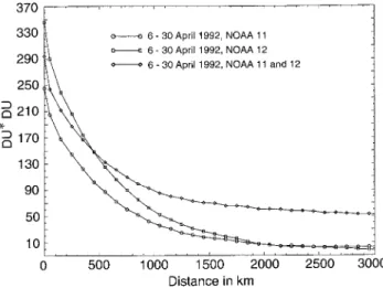
Fig. 3. The error covariance (u0!u")k(u0!u")l averaged for 6 to 30 April 1992
Bergtho´rsson and Do¨o¨s (1955), which is the forerunner of the method of successive corrections (Daley, 1991). In the implementation of the method used here, an analysed ozone field at time t#Dt is obtained by taking a weighted average between the background field at t#Dt and ob-served ozone data obtained between t and t#Dt. For practical reasons the assimilation timestep is the same as the advection timestep in the AMK (Dt"6 min).
Starting from an ozone field at t, a first-guess ozone field at t#Dt is calculated with the advection proce-dure already mentioned. This first-guess field is used as a background field in the data-assimilation procedure. The background ozone field at t#Dt (u") is weighted with observed ozone data (u0) obtained between t and
t#Dt, using only a single correction step. An analysed
ozone map at t#Dt is then obtained. The analysed ozone valueu!i is defined by:
u!i"u"i#¼ik(u0k!u"k). (3) Hereu"i and u"k are background ozone at the gridpoint
i and the observation point k, respectively, andu0k is the
observed ozone at observation point k, ¼ik is a weighting coefficient and (u0k!u"k) is the observation increment. If
K observations are available, then Eq. 3 becomes:
u!i " u"i#+K k/1¼ik(u0k
!u"k), (4) wherein ¼ik are the weighting coefficients which are a priori specified:
¼ik"p20#+Kk/1p2"u(rik)op2"u(rik)o , (5) wherep20 is the observation-error variance, p2" is the back-ground-error variance, rik is the distance between analysis point i and observation point k and o is a correction function.u(rik) contains information about the influence of an observation at point k on the ozone value of the gridbox at point i that is being analysed.u(rik) is assumed to be dependent only on the distance between i and k and has the following properties:
u(rik)"1 when rik"0 and u(rik)P0 if DrikDPR. The weightu(rik) has been determined by several methods. Cressman (1959) and Sasaki (1960) adopted an r-depen-dent function foru(rik), whereas Bergtho´rsson and Do¨o¨s (1955) derived the weight u(rik) statistically from data. In this paper the weights are estimated from the calcu-lation of an error covariance matrix with elements (u0!u")k(u0!u")l, which corresponds to the mean of the product of the differences (u0!u"). It is assumed that the observation error is spatially uncorrelated as well as uncorrelated with the background error. This results in: u0!u")k(u0!u")l "M(u0!ut)!(u"!ut)NkM(u0!ut)!(u"!ut)Nl "Md0kd0l!d0kd"l!d"kd0l#d"kd"lN "p2"k(rkl) for rklO0 and "p20#p2" for rkl"0, (6) whereut is the true ozone value, d0 and d" are the error in the observation and the model, respectively, andk(rkl) is the correlation between background ozone error at the observation points k and l. For the calculation of the elements (u0!u") in the error covariance matrix the advected value at the gridpoint closest to the observation is taken. Furthermore, the covariance is assumed to be only dependent on the distance between the observations, and is thus not a function of their absolute positions or their relative orientation, which means that the correla-tion k is only r-dependent. Thus, calculating the error covariance matrix gives information about the correlation between the error in advected ozone at point k and the error in advected ozone at point l, and as such provides a weightu(rik) for the difference (u0!u")k at observation point k to be applied at gridpoint i (see Eq. 4). In this paper the correlationk(r) is used as the weight u(rik).
The error covariance matrix is calculated by summing over contributions per distance interval rkl, where rkl is the distance between observation points k and l. In the ab-sence of systematic differences between u0 and u", the error covariance should decrease to zero at large distance (rklPR). This reflects the fact that observations which lie far apart from the gridbox being analysed have little influence.
In Fig. 3 the error covariance matrix calculated per distance interval of 100 km is shown. At k"l the error variancep20#p2" is 250 and 350 DU2 for NOAA-11 and NOAA-12 TOVS data, respectively. For determining the coefficientsu(rik) from the covariance matrix we assume that the observation-error variance is equal to the back-ground-error variance (i.e.p20"p2"), which is a reasonable zero-order approximation. The observation-error vari-ance, as well as the background-error varivari-ance, is then 125—175 DU2, resulting in an observation error of 11—13 DU. The error in TOVS observations on the TIROS-N series of satellites is in the order of 15—20 DU
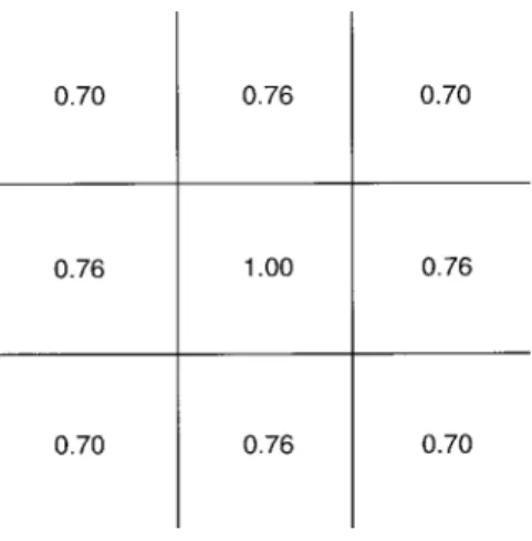
Fig. 4. In the grid boxes the coefficientsk(r)o are shown
(Planet et al., 1984). The error correlationk(r), and thus the weighting coefficientsu(rik), was then obtained after dividing the error covariancep2"k(r) (for rO0) by the error variancep2". Equation 4 can then be written as:
u!i"u"i#+K k/1 k(r"rik)o 1#+K k/1k(r"rik)o (u0k!u"k). (7) The calculation of the error covariance was performed for the entire month April 1992 and the error covariance in Fig. 3 was obtained by averaging over the results from 6 April to 30 April 1992, allowing for a spin-up time of the model of 5 days. The 50-km point in the covariance plot is the average of the contributions obtained in the interval from 1 to 99 km, the 150-km point in the interval from 100 to 199 km, etc. As expected, the covariance is a decreasing function of the distance between observations, becoming negligible after 1500 km. This is consistent with the spatial extent of synoptic weather systems, which are reflected in the ozone field. However, k(rkl) is larger than 1 for
rkl(400 km. This means that the assumption of spatially
uncorrelated observation errors can not be true for this interval, given thatp20"p2". This problem can be solved by taking into account a correction factoro (Bergtho´rsson and Do¨o¨s, 1955). This function can for example be chosen to be the ratio of one over the amount of observations redundant with observation k. We have chosen o to be equal to 0.5.
A radius of 150 km is taken for the circle of influence of an observation. This means that for the grid used in the AMK (100]100 km), weighting coefficients are needed for 100 and 140 km approximately. These distances are based on a simplified representation of the grid as shown in Fig. 4. The coefficients were determined by interpola-tion of the 50- and 150-km values from the error covariance calculated for NOAA-11 data in Fig. 3. With these improved coefficients, the procedure, starting with the calculation of the error covariance matrix for the entire month April 1992, was repeated until the weights no longer changed significantly (which was already after the second iteration). Theu(rik)o"k(r)o thus obtained are 1, 0.76 and 0.70, for distances rkl equal to 0, 100 and 140 km,
respectively, as is shown in Fig. 4. Experiments with slightly different weighting coefficients indicate that the model performance is relatively insensitive to the exact choice of weighting coefficients. Coefficients obtained for NOAA-11 or NOAA-12 data are practically identical.
Assimilating both NOAA-11 and/or NOAA-12 TOVS ozone data resulted in different covariance matrices. The difference when using both NOAA-11 and NOAA-12 data is not yet understood. However, an explanation could be a systematic bias in the order of 6 DU, between NOAA-11 and NOAA-12 total ozone values. If there is a systematic bias between the NOAA-11 and -12 observations, the advected ozone can not be consistent with both types of satellite data. The resulting bias between advected data and observed data is reflected in the error covariance, especially for rklPR.
5 The choice of the wind field
The optimal wind field is determined empirically as the wind field which gives the smallest rms difference between advected-total-ozone and observed-total-ozone data in the timeframe of the advection step:
e"J1/K+Kk/1(u0k!u"k)2k, (8) where K"number of observations, u0k"observed total ozone,u"k"advected total ozone, e"root mean square difference and k"observation.
Wind-field levels used are 50, 70, 100, 200, 250, 300 and 500 hPa. As a test case April 1992 is chosen, because of the high variability of the ozone-field as well as the absence of fast (ozone-hole) chemistry. The initial ozone field is an analysed ozone field, obtained by running the AMK for about 1 year prior to April 1992. In principle 7 days would have been enough to obtain an accurate analysed ozone field as initial field, starting from an uniform ozone field of 300 DU. Experiments with 7-day runs showed that the obtained analysed ozone field, compared with an ozone field constructed by continuous data assimilation, re-vealed only differences between these ozone fields below the 1% level. This means that the difference in rms error e obtained for the two analysed ozone fields diminishes in 30 h to half of its original value. As the AMK is continu-ously used, the initial field was obtained by running the model for about 1 year.
To test the behaviour of the model, gaps of 4 days in the ozone data have been introduced artificially. In this 4-day period the ozone field is only advected, i.e. no observa-tions are used. These ozone-data-deficient periods are followed by a period of 5 days wherein data assimilation uses all available TOVS ozone data in order to recover a realistic total-ozone distribution. This procedure is re-peated three times. The scheme is shown in Table 1. In order to investigate whether different wind fields are needed for transporting total ozone in dynamically differ-ently behaving parts of the atmosphere,e is also calculated separately for the northern hemisphere outside the equa-torial region (30°—90°N), the equaequa-torial region (30°N— 30°S) and the southern hemisphere outside the equatorial
Table 1. Description of data used to test which wind-field level is the optimal choice to run the AMK. As a test case, TOVS data of April 1992 are taken (adv"advection, ass"assimilation)
DATA or GAP Day Hour Day Hour in April (UTC) in April (UTC) DATA (adv#ass) 1 0000 — 3 2400 GAP (adv) 4 0000 — 7 2400 DATA (adv#ass) 8 0000 — 12 2400 GAP (adv) 13 0000 — 16 2400 DATA (adv#ass) 17 0000 — 21 2400 GAP (adv) 22 0000 — 25 2400 DATA (adv#ass) 26 0000 — 30 2400
Fig. 5. The rms-differencee of advected TOVS data compared to raw TOVS data (see Eq. 6) for the total globe, calculated for a wind field at the pressure levels 50, 70, 100, 200, 250, 300 and 500 hPa
Fig. 6. As in Fig. 5 but only for the NH region (30°—90°N)
Fig. 7. As in Fig. 5 but only for the SH region (30°—90°S)
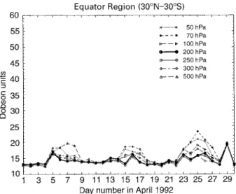
Fig. 8. As in Fig. 5 but only for the EQ region (30°N—30°S)
region (30°—90°S), which are noted as the NH, EQ and SH region, respectively.
In Figs. 5—8, values ofe for all wind fields, for the NH, EQ and SH regions, and averaged over the whole globe, are presented. An oscillating structure in e is easily
denoted, which is caused by the artificially produced data gaps. During periods without data assimilation, e in-creases sharply until it stabilises after 2 days (4—7, 13—16 and 22—25 April). As soon as new satellite data are intro-duced by data assimilation,e decreases and also stabilises after 2 days (8—12, 17—21 and 26—30 April). Thus the global ozone map is recovered after 3 days of advecting and assimilating satellite data. The increase in e is most ex-treme in the NH region (between 20 and 58 DU), and much smaller on the SH region (between 15 and 33 DU) and at the EQ region (between 13 and 25 DU). Between the different latitude bands in the NH, 30—50 N, 50—70 N and 70—90 N, no significant difference ine is found (not shown). The high sensitivity upon the right choice of wind field in the NH region is caused by the greater spatial and temporal variability in the ozone field during winter and spring in the NH region than in the EQ region and, to a lesser extent, in the SH region. This will result in a higher sensitivity upon the choice of wind field for the NH region compared to the EQ and SH regions.
The 200- or 250-hPa wind-field levels are clearly the best pressure-level wind fields for transporting column
amount of ozone, followed by the 300-hPa wind-field level. This is true for the global, NH, SH and EQ calcu-lations (see Figs. 5—8). This confirms that the maximum variability is indeed around and above tropopause level, which is between 200 and 300 hPa in the NH at mid-latitudes.
Similar results are also found by Riishøjgaard and Lary (1994). They studied the correlation between the forecast error for total ozone and the forecast error for geopoten-tial height at 50, 200, 500 and 850 hPa in the northern-hemisphere extratropics. The geopotential height error near tropopause level (200 hPa) showed the stron-gest correlation.
6 Discussion and conclusions
The two-dimensional model, AMK, for advection and assimilation of total-ozone satellite data using a wind field at a single pressure level, has been presented. The model is powerful for assimilating satellite data, even, for example, for satellites with a narrow swath width, such as GOME, or satellite data with gaps due e.g. to retrieval problems, as is shown in this study using TOVS data. By alternating periods of 4 days of only advection and no data assimila-tion with periods of 5 days of advecassimila-tion and assimilaassimila-tion, it can be concluded that the 200-hPa wind-field level is a good choice of wind field to advect total-ozone-column data. Using a different approach the same wind-field level was also found by Riishøjgaard and Lary (1994). Consid-eration of atmospheric dynamics permits a first under-standing why this wind field should be used for advecting total ozone. Successive satellite measurements of total ozone detect changes in the ozone column amount, which is the resultant of ozone transport by different winds at different levels. If the ozone concentration is uniform over the globe, no changes in column amounts would be vis-ible. Since high-pressure regions correspond to low ozone values and low-pressure regions to high ozone values (Dobson, 1968), meteorological features appear to be clearly distinguishable in the total-ozone field. These high-and low-pressure regions are accompanied by substantial fluctuations in the tropopause height. Moreover there is a strong vertical gradient in the ozone mixing ratio just above the tropopause. The synoptic scale changes in total ozone are thus expected to be caused by changes in the ozone distribution around the tropopause level. It is therefore reasonable to assume that wind fields at pressure levels around the tropopause are representative wind fields to describe the transport of column amount of ozone. As was shown, the most simple choice of transport by a wind field at a single pressure level already gives a reasonable description of the transport of the column amounts of ozone. Vertical velocities near the tropopause will also lead to changes in total ozone. In this study the effects of vertical motions have been neglected. In the atmosphere both mechanisms are expected to contribute to the variability of total ozone. The small rms differences, e, found in this study suggest however, that changes in column amounts of ozone due to horizontal motions are more important than those due to vertical motions.
The model is also used for validating the GOME in-strument measurements (Piters et al., 1996). Validation of satellite data by ground-based measurements is impor-tant, especially for long-term trend detection, ozone cli-matology and intercomparison of data measured by dif-ferent satellites. However, ground-based measurements taken at different times and different geographical loca-tions from the satellite measurements are less suited for direct comparison. Also, satellite measurements usually represent averages over a large area, whereas conven-tional measurements represent local values, which makes the two not directly comparable. The AMK, which retains the dynamical information on ozone, makes it possible to use also these non-collocated measurements for valida-tion. Moreover, data assimilation offers the possibility to identify ground stations which deliver controversial data by comparison with observations of a satellite instrument. This model is a first attempt to advect and assimilate total-ozone data and can be improved in several ways. A time-interpolated wind field between the 3-, 6- and 9-h forecasts can be used, instead of taking a fixed wind field during a 6-h period. Moreover, other wind fields could be taken into account. A combination of wind fields at differ-ent heights would be an obvious choice. This would be a first step towards a three-dimensional approach. For ozone-profile satellite data a three-dimensional approach, as was already shown by Riishøjgaard (1995) and Swin-bank and O’ Neill (1994), is needed. However, it should be mentioned that the two-dimensional approach in the AMK is very useful, because most satellite instruments available produce high-quality measurements of column amounts of ozone and considerably less profile informa-tion of ozone. The data-assimilainforma-tion technique used in our model is a first step and will be improved by extending the radius of influence of the observations (currently 150 km). More elaborate data-assimilation methods, such as Opti-mal Interpolation or four-dimensional variational tech-niques (Daley, 1991), will be needed when other tracers are also taken into account, or when one wants to extract dynamical information from the ozone field. Some of these different aspects will be considered in the near future. Acknowledgements. The research of P. F. L. has been funded by the
Beleidscommissie Remote Sensing (BCRS). We thank NOAA NES-DIS, NASA and ECMWF for making available the TOVS data, TOMS data and MARS archive data, respectively. We thank Ad Stoffelen and Elı´as Ho´lm for many interesting discussions and contributions, especially on the subjects of data assimilation and advection. We thank the referees for their valuable comments.
Topical Editor F. Vial thanks R. Swinbank and L. P. Riishøjgaard for their help in evaluating this paper.
References
Allaart, M. A. F., H. Kelder, and L. C. Heijboer, On the relation between ozone and potential vorticity, Geophys. Res. ¸ett., 20, 811, 1993.
Bergtho´rsson, P., and B. R. Do¨o¨s, Numerical weather map analysis, ¹ellus, 7, 329, 1955.
Cressman, G., An operational objective analysis system, Mon. ¼eather Rev., 87, 367, 1959.
Daley, R., Atmospheric Data Analysis, Cambridge University Press, Canada, 1991.
Danielsen, E. F., Ozone transport, in Ozone in the Free Atmosphere, eds. R. C. Whitten and S. S. Prasad, Van Nostrand Reinhold, New York, pp. 123—159, 1985.
Dobson, G. M. B., Forty years’ research on atmospheric ozone at Oxford: a history, Appl. Opt., 7, 387, 1968.
Dobson, G. M. B., D. N. Harrison, and J. Lawrence, Measurement of the amount of ozone in the Earth’s atmosphere and its rela-tion to other physical condirela-tions, Proc. Roy. Soc., A122, 456, 1928.
ESA Document, Mission Objectives, User and System Requirements for an Ozone Monitoring Instrument on METOP, in press, 1996 Hahne, A., J. Lefebvre, J. Callies, and R. Zobl, GOME: a new
instrument for ERS-2, ESA Bulletin, 73, 22, 1993.
Heath, D. F., A. J. Krueger, H. A. Roeder, and B. D. Henderson, The solar backscatter ultraviolet and total ozone mapping spectrometer (SBUV/ TOMS) for NIMBUS G, Opt. Eng., 14, 323, 1975.
Heijboer, L. C., H. Kelder, M. J. M. Saraber, and P. F. J. van Velthoven, An analytical model describing the basic structure and development of mature extratropical cyclones, accepted for
publication in Mon. ¼eather Rev., 1996.
Lary, D. J., M. P. Chipperfield, J. A. Pyle, W. A. Norton, and L. P. Riishøjgaard, Three-dimensional tracer initialization and general diagnostics using equivalent PV latitude-potential-temperature coordinates, Q. J. R. Meteorol. Soc., 121, 187, 1995.
Levelt, P. F., and M. A. F. Allaart, Two-dimensional advection model for interpolation of ozone satellite data, Proc. of SPIE
Atmos. Sensing and Modelling, 29—30 Sept. 1994, Rome, Italy.,
2311, 217, 1994.
Piters, A. J. M., P. F. Levelt, M. A. F. Allaart, and H. M. Kelder, Validation of GOME total ozone column with the assimilation model KNMI, GOME Geophysical Validation Campaign, Final Results, Workshop Proceedings, held by ESA-ESRIN in Frascati 24—26 January 1996.
Planet, W. G., D. S. Crosby, J. H. Lienisch, and M. L. Hill, Deter-mination of Total Ozone Amount from TIROS Radiance Measurements, J. Clim. Appl. Meteorol., 23, 308, 1984. Riishøjgaard, L. P., On four-dimensional variational assimilation of
ozone data in weather prediction models, accepted for publication
in Quart. J. Roy. Meteor. Soc., 1995.
Riishøjgaard, L. P., and D. J. Lary, Short-range simulations of extratropical total ozone with APERGE/-IFS, Proc. of ECM¼F ¼orkshop on the stratosphere and numerical weather prediction, ECMWF, 1994.
Rood, R. B., Numerical advection algorithms and their role in atmospheric transport and chemistry models, Rev. Geophys., 25, 71, 1987.
Sasaki, Y, An objective analysis for determining initial conditions for the primitive equations, ¹ech. Rep. (Ref. 60-16T) (College
Station: Texas A&M University), 1960.
Smith, W. L., H. M. Woolf, C. M. Hayden, D. Q. Wark, and L. M. McMillen, The TIROS-N operational vertical sounder, Bull. Am.
Meteorol. Soc., 60, 1177, 1979.
Stolarski, R. S., P. Bloomfield, and R. D. McPeters, Total ozone trends deduced from Nimbus 7 TOMS data, Geophys. Res. ¸ett., 18, 1015, 1991.
Swinbank, R., and A. O’Neill, A stratosphere-troposphere data as-similation system, Mon. ¼eather. Rev., 122, 686, 1994.
.