HAL Id: hal-02307211
https://hal.archives-ouvertes.fr/hal-02307211
Submitted on 7 Oct 2019HAL is a multi-disciplinary open access archive for the deposit and dissemination of sci-entific research documents, whether they are pub-lished or not. The documents may come from teaching and research institutions in France or abroad, or from public or private research centers.
L’archive ouverte pluridisciplinaire HAL, est destinée au dépôt et à la diffusion de documents scientifiques de niveau recherche, publiés ou non, émanant des établissements d’enseignement et de recherche français ou étrangers, des laboratoires publics ou privés.
Comparison of Equivalent Conductivities for Numerical
Simulation of One-Dimensional Unsaturated Flow
Benjamin Belfort, François Lehmann
To cite this version:
Benjamin Belfort, François Lehmann. Comparison of Equivalent Conductivities for Numerical Simulation of OneDimensional Unsaturated Flow. Vadose Zone Journal, Soil science society of America -Geological society of America., 2005, 4 (4), pp.1191. �10.2136/vzj2005.0007�. �hal-02307211�
COMPARISON OF EQUIVALENT
CONDUCTIVITIES FOR NUMERICAL SIMULATION OF
ONE-DIMENSIONAL UNSATURATED FLOW
Benjamin Belfort and François Lehmann
Institut de Mécanique des Fluides et des Solides UMR 7507 ULP-CNRS
2 rue Boussingault, Strasbourg, France. E-mail: [email protected]
Submitted to Vadose Zone Journal - January 2005 Revised Manuscript April 2005
Abstract
Water flow in unsaturated porous media is usually simulated using the Richards equation in combination with some numerical method for spatial and temporal discretization. In this study we implement a mixed hybrid finite element solution with different formulations for the equivalent hydraulic conductivity in an attempt to more accuratly simulate variably-saturated flow. The advantages of a quadrature rule are demonstrated for simulations of sharp infiltration fronts. Results show the importance of selecting an appropriate equivalent conductivity. Geometric, weighted and integrated formulations produced better solutions than a traditional scheme using a mean conductivity calculated with a mean pressure head. Two illustrative test cases are considered for infiltration in initially dry homogeneous and heterogeneous soils subject to both Dirichlet and variable Neumann boundary conditions. The accuracy and computational efficiency of the proposed algorithm with the different conductivity formulations is demonstrated by means of comparisons with a finite difference approach using various interblock conductivity averages.
Accurate numerical simulation of infiltration in initially dry porous media remains a challenge, especially when very sharp fronts are present (Milly, 1985 ; Pan et al., 1996). Numerical techniques for solving the governing variably-saturated flow equation are typically implemented on either a fixed or adaptative spatial grid (Mansell et al., 2002). In this study we assume a pre-generated fixed grid and try to improve the numerical solutions by introducing more effective interpolation rules to produce a better conditioned matrix system and representative equivalent parameters, rather than resorting to very small meshes. A finite difference (FD) scheme involving mesh-centered grids for the Dirichlet boundary conditions and block-centered grids for flux controlled condition will be used.
Various formulations have been proposed in the literature to more accurately estimate FD relative conductivities between adjacent nodes, often referred to as interblock or internodal permeabilities. These permeabilities are most commonly approximated using arithmetic, geometric and harmonic means of the conductivities of the two neighbouring elements (Haverkamp and Vauclin, 1979 ; Schnabel and Richie, 1984). Other schemes such as integral averages of the conductivity (e.g., the Kirchhoff integral method; Zaidel and Russo, 1992), Darcian averages (Warrick, 1991 ; Baker, 1995) or weighted averages (Gasto et al., 2002) have also been implemented successfully. Despite the promising results reported by the different authors, these schemes have not been widely adopted because of the additional complexity and/or computational effort involved. Moreover, little information exists about the treatment of interblock conductivities when the two neighbouring nodes are located in soil layers with contrasting hydraulic properties (Zaidel and Russo, 1992 ; Brunone et al., 2003), a situation which is commonly encountered in the field. The accuracy of unsaturated flow predictions may then very much depend on how interlayer conductivities are evaluated.
This study is focused principally on an alternatively numerical approach referred to in the literature as the mixed hybrid finite element (MHFE) method (Chavent and Roberts, 1991).
MHFE schemes simultaneously approximate both the pressure head and its gradient; they have been generalized for variably-saturated flow and analyzed in terms of the temporal approximation involved (Farthing et al., 2003), the adopted linearization technique (Bergamaschi and Putti, 1999) or for adaptative grid refinement (Bause and Knabner, 2004). Similar to the conventional mass-distributed finite element (FE) method, the MHFE approach suffers from numerical oscillations when sharp infiltration fronts are simulated.
The paper begins with a brief description of unsaturated flow theory and the MHFE method. Alternative formulations used to improve the estimation of the hydraulic conductivity are then presented. This part is followed by explanations of quadrature rule implemented for eliminating oscillations. Next these aspects are illustrated by two test cases involving different materials and boundary conditions. While our focus was on the MHFE method, results may be useful also for improving related finite difference formulations.
ONE-DIMENSIONAL UNSATURATED WATER FLOW
Darcy’s law for saturated flow as generalized by Buckingham for unsaturated vertical flow (Narasimhan, 2004) is given by
q K h . h z [1]
where q is the macroscopic fluid flux density, K is the hydraulic conductivity, h is the pressure head and z is the depth taken to be positive downwards. One-dimensional vertical fluid flow in variably saturated porous media, including the effects of specific storage, is given by the following mixed form of the Richards equation:
s w v h h S S .q f t t [2]where is the volumetric water content, t is time, Ss is the specific storage coefficient, Sw
(=/s) is relative saturation of the aqueous phase (s is the saturated water content), fv is a
source/sink term, and q is given by Eq. [1].
NUMERICAL METHODS
The FD and MFHE numerical techniques to be compared in this study were implemented using the same temporal approximation and the same linearization technique. Temporal discretization was accomplished using a backward Euler (fully implicit) scheme with either a fixed time step or an empirical automated self-adjusting time stepping approach. Time steps were adjusted based on the number of iterations needed to reach convergence. A modified Picard iteration scheme was used for linearization of the discretized flow equation, while the final set of differential algebraic equations was solved using the Thomas algorithm. In this section we describe in detail the MHFE method as programmed and tested. We first briefly review the traditional MHFE approach (Chavent and Roberts, 1991), and then focus in particular on the new features that were implemented.
The MHFE method provides simultaneous approximations of both the pressure head and the fluid flux, which are calculated throughout the domain. The numerical scheme is based on a Raviart-Thomas finite element discretization of degree zero (RT0; Raviart and Thomas,
1977) using classic scalar and vector basis functions. For a flow domain made up of Ne
elements ei , these basis functions ( et ei) over element ei are given by
1 Ne i i e ; 1
1
1 1 i i i i i i i i i z z z z z e z ,z z z z z ; 1 0 i i e on element e elsewhere [3]The pressure heads and fluxes are then estimated by 1
i i Ne e e i h h and 1
Nn j j j q q [4]where Ne and Nn are the total number of elements and nodes, respectively.
Assuming that the hydraulic conductivity K is not equal to zero, the variational formulations of Darcy-Buckingham’s law [1] and the Richards equation [2] are given by (Brezzi and Fortin, 1991):
1 1
K q. jd
h. jd
z. jd j ,..., Nn [5]
1
ei
s w ei
ei
v ei h d S S d .q d f d i ,..., Ne t t [6]The properties of the basis functions leads to the following equation for [6]:
1 1 1 1 i i i i i i i i i n n n n e e n e e e s w,e e ,i e ,i v ,e h h z S S ( q q ) f t t [7]
in which qei,i and qei,i+1 are outward fluxes at the boundaries of element ei of length zei.
The application of Green’s formula to Eq. [5] and introducing Lagrangian multipliers (or traces of the pressure head, Thj) that represent the pressure head at nodal points in one
dimension leads to
1 1 2 2 i i i i i i i e e i e ,i e e e ,i e i z h Th q A . z q h Th [8] in which
1
i i i , j i j e e A A K dz [9]For node i between the elements ei-1 and ei, the flux continuity equation may be written as
1 0
i i
e ,i e ,i
q q [10]
The following steps form now part of the MHFE hybridization process:
1. Equation [8] provides expressions of the nodal fluxes as a function of the mean pressure head and the traces of the pressure head, i.e., q f h,Th
2. Following Celia et al. (1990), the water content in Eq. [7] is expanded by means of a first-order Taylor series with respect to h to obtain an expression for the mean pressure head, i.e., h f Th
3. Mean pressures resulting from step 2 are used in the expression of fluxes given in step 1, which is then substituted into Eq. [10] at each interface between elements of the domain. Traces of the pressure head are the main unknowns and are calculated at each step time with the resulting tri-diagonal matrix equation.
We now consider several alternative methods for calculating the matrix [A]ei related to the
scalar product of the basis functions. We first focus on how the conductivity in Eq. [8] is best evaluated. As with previous saturated flow studies, most current approaches for variably saturated flow assume a mean conductivity approximated over each element using the mean pressure, i.e.,
i i
e e mean
K K h K . Another approach suggested in this study is to introduce various averages to calculate this equivalent conductivity, which is then also assumed constant over each element. Since the mean pressure head and the traces of the pressure head are known for each element, the mean conductivity values are readily calculated (Table 1). The integrated mean values were numerically evaluated using a five point Gauss-Legendre
quadrature scheme. The weighted mean conductivities (Gasto et al., 2002) were calculated using weighting factors () that are functions of the nodal spacing, the parameter n of the
invoked soil hydraulic property model and the conductivities at the two nodes of each element. This algorithm required 8 constants as discussed by Gasto et al., (2002).
Another aspect of Eq. [9] is the scalar product ( i.j ), which can be calculated either
exactly or in an approximate manner. Farthing et al (2003) reported that exact calculations may lead to oscillations, especially when sharp infiltration fronts are present. An analysis of the matrix system shows that a criterion depending upon nodal spacing and the time increment may condition adherence to the discrete maximum principle for the pressure head solution:
2 6 i i i e e e s w ,ei z K t C S S [11]This criterion [11] is similar to that used for saturated flow without specific storage (Hoteit et al., 2002), but with the important difference that the conductivity Kei and the soil moisture
capacity Cei are now variable, which makes the condition very restrictive.
Additionally, a quadrature rule can be used with the MHFE method (Chounet et al., 1999 ; Farthing et al., 2003) to estimate the matrix [A]ei by taking advantage of the mass-lumping
procedure introduced by Neuman (1972) for the FE method. The quadrature rule is given by
1 1 1 2
i i i e ij i j i i j i i i j i e e z A K . . dz z . z z . z K ij [12]Using this quadrature rule and following the procedure described above leads to
1 1 1 1 1 1 1 1 1 1 1 1 1 1 1 1 2 2 i i i i i i i i n ,k n ,k e e n ,k n ,k n ,k n ,k n ,k n ,k i e e e e i n ,k n ,k e e i K . Th K K . Th z z K . Th z 1 1 1 n ,k n ,k i R [13]which represents flux continuity at node i between elements ei-1 and ei. In Eq. [13] 1 1 1 1 n ,k n ,k n ,k Th Th Th [14]
1 1 1 1 1 1 1 1 1 1 1 1 1 1 1 1 1 1 1 1 1 1 1 1 1 1 1 2 2 2 i i i i i i i i i i i i i n ,k n ,k e e n ,k n ,k n ,k n ,k n ,k n ,k n ,k i i e e e e i n ,k n ,k e e n ,k n ,k n ,k n ,k n ,k n ,k i e e e e e e K R .Th K K .Th z z K .Th K K K K z z
1 i n ,k [15]
1 2 1 1 1 1 1 4 i i i i n ,k n ,k e s w,e n ,k e n ,k e z C S S K t [16] 1 1 1 1 1 1 1 4 i i i i i i i i i i n ,k n ,k n n ,k n ,k n ,k n e e e e e s w,e e e n ,k e n ,k v e z. C h S S h z f K t [17]The global matrix system is obtained by writing Eq. [13] for all nodes of the domain. We note here that the coefficient
i
n 1,k e
takes on values between 0 and 1, which causes the off-diagonal coefficients of the matrix equation to become negative. This means that the resulting numerical fluxes are physically consistent and that oscillations are eliminated from simulations with sharp wetting fronts (Hoteit et al., 2002).
Another interesting approach that we tested is a global common quadrature scheme (referred to as “GlobQ” in Fig. 3) for the conductivity and the scalar products:
1
1 1 2 i e i i j i i i j i ij i i z z . z z . z A K z K z [18]The following three MHFE schemes are hence evaluated in this study:
1. A classical scheme with a quadrature rule to calculate the equivalent conductivity. 2. One quadrature rule for the scalar product of the basis functions and another
quadrature rule for the equivalent conductivity.
When a flux-controlled condition is applied to the soil surface after a long dry period, the pressure head of the first node can sometimes produce physically unrealistic values. This problem does not seem to depend on the applied boundary value; for example, the approach used by van Dam et al. (2000) does not show any overshooting of the maximum soil water flux at the soil surface. Irrespective of such overshooting, the problem occurs only at the first node, with pressure heads in the remaining part of the domain being unaffected. Actually, since the conductivity increases only gradually upon infiltration, adherence to the flux continuity equation requires that the first node has a large pressure gradient, which can be obtained only by having a very high (negative) pressure head at the first node. We note that MHFE methods do not use the pressure head of the first node, and that the conductivity of the first element is defined using the mean pressure. By comparison, FD methods provide only a mean pressure head for the entire element at the soil surface.
A complete description of the classical FD method that we used for the comparisons can be found in Celia et al. (1990). Since the modified Picard iteration scheme is discussed at length in the literature, we provide here only details that are relevant to our applications. Celia et al. (1990) showed that the spatial derivatives in the FD and FE (with mass-lumping) approximations are identical when the arithmetic mean is used to define the internodal permeability. Table 2 lists the various averaging techniques for simulating unsaturated flow in homogeneous media. Given the conductivity, the flux between two adjacent nodes is simply estimated using Darcy’s law as
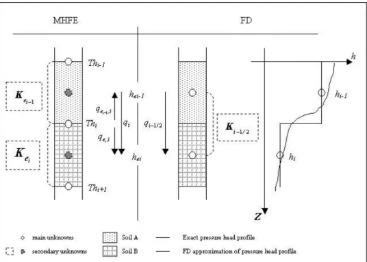
1 2 1 2 1 i / i / i i K q h h z z [19]The various formulations were tested in conjunction with the MHFE scheme. The integrated and weighted formulations required modifications when the interblock conductivity involves two neighbouring elements with different hydraulic properties (see Fig. 1). We used for this purpose a procedure that generalizes the approach reported by Romano et al. (1998). Given
that an implicit scheme was also used for the equivalent conductivity, their method can be simplified to give 2 eq K K K K K with 1 2 1 2 i / ,SOIL A i / ,SOIL B k K k K [20]
in which K+ and K- are the equivalent homogeneous conductivities evaluated using either the properties of the upper soil layer, or those of the lower layer, without introducing fictitious (extrapolated) pressure head values.
CONSTITUTIVE RELATIONSHIPS
The governing flow equations must be solved subject to the Dirichlet or Neumann boundary conditions at both the top and bottom of the soil profile. These conditions are given by
0,t h t0
h or 0
0 1 z h K q t z [21]
L
h L,t h t or 1
L z L h K q t z [22]for the upper and lower boundaries, respectively, where h0 (t) and q0 (t) are the prescribed
pressure head and net flux at the soil surface and hL (t), qL (t) those at the bottom of the profile.
To complete the mathematical description for variably saturated flow, the interdependencies of the pressure head, the hydraulic conductivity and the water content must be characterized using constitutive relations. The standard van Genuchten model (1980) was used here for the pressure - saturation relationship as follows
1 1 0 1 1 0 / n n r e s r 1 h h S h h h [23]where s and r are the saturated and residual volumetric water contents, respectively, is a
parameter related to the mean pore size and n a parameter reflecting the uniformity of the pore-size distribution. Mualem’s model (1976) was chosen for the conductivity - saturation relationship, leading to (van Genuchten, 1980) :
1 1 2 1 1 2 1 1 / n n / n / e s e e K S K S S [24]in which Se is given by Eq. [23] and n > 1.
RESULTS AND DISCUSSION
The effectiveness of the proposed formulations for the equivalent conductivity in the MHFE method was analysed by means of two test cases. We also compared results with different formulations of the FD interblock conductivity. The first test case involves infiltration into an initially dry porous medium, while the second experiment deals with infiltration in, and subsequent evaporation from, a layered soil profile.
Infiltration under a constant head boundary condition
We first consider a problem previously investigated by Celia et al. (1990) for infiltration in a homogeneous porous medium. The relevant material properties are given in Table 3 (Medium A). The initial pressure head h(z,0) of the 100-cm long soil column was assumed to be -1000 cm. Constant pressure head conditions were assigned to both the top (-75 cm) and the bottom (-1000 cm) of the column. As the nodal spacing and the time increment decreased, all formulations combined with the FD or the “mass-lumped” MHFE schemes converged to the same solution. This solution has been assumed to be the correct solution, which coincided
also with the quasi-analytical solution developed by Philip (1957). Several comparisons were performed using a constant time step of 0.1 s and a node spacing of 0.1 cm for the fine grid solution.
A comparison of the various formulations implemented in the classical scheme is shown in Fig. 2 for a nodal spacing of 1 cm and a constant time increment of 20 s. To obtain a good visual comparison of the various schemes, results are given only for the upper 35 cm of the soil profile, while also omitting the region between 10 and 20 cm. All standard MHFE methods were found to produce oscillations. For this test case the criterion (Eq. [11])
introduced previously can be rewritten as
2 4 1 z 2.4 10 cm.s t
. For a nodal spacing of 1 cm
this means that a minimum step time of 1.15 hour should theoretically be selected in order to respect the maximum principle. Other relevant issues are convergence of the modified Picard method and the precision with which the location of the wetting front is predicted. The quadrature rule was found to be very efficient for eliminating the oscillations. However, the locations of the wetting front depended also on the scheme used for the equivalent conductivity.
We now provide results showing how the different averages affected the FD and MHFE simulations. Results are compared in terms of the relatively pressure head error (PE) given by
0 0
z L cal ref z z L ref z z h z dz PE z dz h h [25]where hcal is the pressure head calculated with a particular scheme, and href is the reference
pressure head obtained with a very fine grid system. Fig. 3 shows PE values for various meshes sizes (from 1 to 5 cm) versus CPU time after 6 hours of infiltration. Errors greater than 20% were obtained for the K , K and K formulations in the MHFE scheme, and
for Kharm used with FD. The nodal spacing largely controlled the precision of the solution
between 0.1 and 1 cm. The error changed only slightly for larger nodal spacing. The Kdown, Kharm and Kmean averages favored the lower conductivity and hence underestimated the
equivalent conductivity, thus causing underpredictions of the infiltration rate. While global quadrature similarly underpredicted the flow rate, the accuracy of this scheme actually worsened when the nodal spacing increased (from 4% to 18%). Solutions obtained with Kup
were found to be very sensitive also to the nodal spacing. Unlike the other formulations, the wetting front in this case was overpredicted. Arithmetic, integrated, weighted and geometric means had errors less than 7.5%; the precision was particularly good for these last three averages.
The three most accurate averaging schemes implemented in the MHFE method required about twice as many iterations per time step than the corresponding FD interblock conductivities. This is because the MHFE schemes involve twice as many unknowns as the FD methods, and consequently run more slowly for a given spatial discretization. For the geometric mean, the MHFE scheme required about 15% more CPU time, whereas the integrated and weighted formulations required 17% and 27% more time, respectively. The additional effort did not lead to a similar improvement in the results; still, the integrated and weighted averages remained competitive compared to the traditional arithmetic average FD approach. Comparison of diagrams a°) and b°) in Fig. 3 shows that the geometric mean MHFE scheme provided the best results, followed by the weighted average FD scheme.
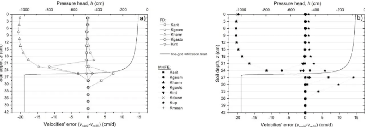
A comparison of errors in the average pore water velocity (v = q / ) is shown in Fig. 4 for
a 3 cm uniform grid. Results are given down to a depth of 42 cm. The velocity error was simply calculated as vcal(i)-vref(i). We used the pore water velocity since this parameter is
frequently used for transport calculations. The efficiency of the various formulations followed the same trend. The Kint and Kgasto averages produced the most efficient solutions, especially
when used in conjunction with FD. This first test case also confirmed a result previously noted by Warrick (1991) in that the geometric mean underestimates fluxes before the infiltration front, whereas the arithmetic mean overpredicts those fluxes.
When the quadrature rule is employed, and using the fluxes qei-1,i and qei,i and flux
continuity equation [10], the fluid flux density obtained with the MHFE method can be written in the form:
1
1 1 2 i i i i i i e e i e e e e K K q h h z z K K This shows that the traditional mean conductivity Kmean hence leads to the same expression as
the FD flux when the harmonic average is used (Chavent and Roberts, 1991), which may explain the relatively poor results shown in Fig. 3b and 4b. Likewise, results with the MHFE harmonic and downstream averages did not improve in that the conductivity was still underestimated or even worsened. Our results also show that a particular averaging scheme may not necessarily have the same effect on the pressure head and the velocity field. For instance, the geometric mean provided very good results for the pressure head, but was far less accurate for the flux; the reverse was the case for the integrated and weighted conductivity averages.
Infiltration, drainage and evaporation into a layered soil
The second test case was used to compare the best formulations for the equivalent conductivity. We considered a soil profile containing five 25-cm thick layers alternatively made up of Berino loamy fine sand (the 1rst, 3rd and 5th layers) and Glendale clay loam (the 2nd
and 4th layers) (Hills et al., 1989). The hydraulic parameters of the Berino and Glendale soils
bottom of the column and a variable flux at the soil surface comprising first rainfall, followed by redistribution/drainage and then evaporation:
0 0 4 2
q t d cm / d;q0
4 t 6d
0 cm / d and q0
6 t 7d
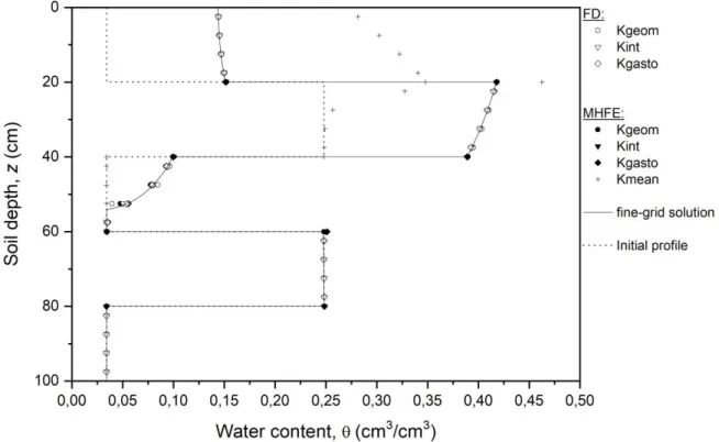
0 3. cm / dGiven the variable soil materials, the high nonlinearity of the corresponding constitutive relationships and the changing boundary conditions at the soil surface, this case should be a good test of the accuracy of the various numerical schemes. With a nodal spacing of 0.1 cm, all solutions computed with the different formulations gave the same profile. Results obtained with this fine grid hence will be used as the reference solution. Results were obtained with the FD and MHFE methods using integrated, weighted and geometric conductivity averages. We also simulated the problem using a traditional MHFE mean conductivity function, Kmean. A
nodal spacing of 5 cm was selected for the comparisons.
Figure 5 shows calculated soil water content profiles after 3 days of infiltration. Also shown are the fine-grid solution and the initial condition. We note here that the calculated trace of the pressure head (for the MHFE method) can be used to estimate water contents on both sides of an interface between two different layers. This is not immediately possible with the FD method. The numerical results in Fig. 5 confirm the difficulties of using the mean conductivity MHFE scheme for the relatively large grid size (5 cm) selected: infiltration was relatively slow, with the wetting front reaching only the top of the third layer. The mean conductivity MHFE scheme similarly limits the evaporation rate. The other formulations all gave satisfactory results for the water content profile; very similar results were obtained at several other times during the simulations (further results not shown here).
Figure 6 shows calculated flux errors at each layer interface for the different averaging schemes (the left vertical axis of each plot). The figures also show the fine-grid solution for the flux itself (solid lines) associated with the axis on the right side of each plot, but all with different scales to improve visual presentation of the results. The wetting front reached the
fourth layer after 4 days. The fluxes at the first three interfaces increased rapidly to above 1 cm/d. It should be noted that the flux errors were much smaller at the second and fourth interfaces (Fig. 6 b, d). This finding can be explained by considering that the conductivities of the upper and lower layers change as a function of saturation. Initially, material C was more than 100 times more conductive than material B (KC 9 0 10. 4 cm/d;
6
7 0 10
B
K . cm/d), whereas the opposite occurs above a pressure
head of about -130 cm. In fact, the water content and hydraulic conductivity characteristics have sharper saddles (a higher n value) for the fine sand (material B) as compared to the more fine-textured material C, which causes the infiltration processes to be different in the two types of soil layers. The flux at each interface is controlled in part also by the dynamics in the upper layer. The result is that the flux increases much more rapidly at the first and the third interfaces (Fig. 6), with concomitantly much larger flux errors at these interfaces.
Figures 6a and 6c show relatively similar evolutions of the flux error. The MHFE integrated and weighted averages produce results that are slightly ahead of the fine-grid solution; the advance of the wetting front is more diffusive and the maximum flux is not reached quickly. These averages slowly produce better results such that after about 2.5 days the flux errors have become very small (e.g., Fig. 6a). Improvements for the third interface took more time because of continuing changes in the flux itself. The FD Kint and Kgasto
formulations performed better when the flux increased sharply. However, the performance of these two schemes was relatively worse when the boundary condition changed, especially during evaporation (Fig. 6a). The FD geometric formulation provided erroneous results when the flux changed slowly, for instance at the beginning and during the second part of the experiment, whereas the corresponding MHFE mean approach was more accurate during the entire simulation.
Figures 6b and 6d confirm the above results. The flux at the interfaces increased or decreased more slowly, while the integrated and weighted means were very accurate. The geometric formulation gave the best results when combined with the MHFE method.
SUMMARY AND CONCLUSIONS
This study was undertaken to analyse the effects of various formulations for the equivalent conductivity in a MHFE model for simulating variably-saturated flow. Numerous simulations involving infiltration in homogeneous and layered soil profiles were carried out and compared with FD schemes that incorporated different expressions for the interblock conductivity. Our numerical investigations permit the following conclusions:
1. For highly nonlinear conditions corresponding to infiltration in initially dry porous media, classical MHFE solutions produce undesired oscillations. Using smaller nodal spacing and adjustment of the time step can improve simulations of the infiltration front. However, it is difficult to simultaneously satisfy both the maximum principle criterion and convergence of the linearization method. The quadrature rule provided an efficient method for eliminating oscillations.
2. When large nodal spacings are used, results obtained with the traditional mean conductivity can be improved significantly by using geometric, weighted or integrated averages. Harmonic and downstream means underestimate the infiltration front, whereas arithmetic or upstream averages overestimate the location of the wetting front, similarly to their FD counterparts. The common quadrature rule failed to produce better results. Suitable estimation of the equivalent hydraulic conductivity is essential for accurate simulations of unsaturated flow.
3. The MHFE method does not need special modifications for modeling layered soil systems. In this case, the limitation consists in considering homogeneous material in each element. This method automatically generates velocity fields throughout the flow domain, while flux continuity is always satisfied at textural interfaces.
4. The proposed model hence gives very attractive solutions. While less satisfactory when implemented in FD schemes, the geometric mean MHFE scheme appears very promising in terms of both accuracy and computational efficiency. And although the integrated formulations are also very accurate, their insertion in existing models is less straightforward and requires more CPU time. The weighted average could represent an interesting alternative; we recommend its further use since the FD geometric mean has been shown to perform relatively poorly in some cases (Zaidel and Russo, 1992; van Dam and Feddes, 2000; Gasto et al., 2002).
While accurate and robust FD solutions have been proposed (Brunone et al., 2003), the geometric, integrated and weighted MHFE formulations may prove to be very attractive for relatively difficult situations such as those involving extreme variations in saturation and subsurface heterogeneity. In fact this study has shown how the MHFE model can be made less dependent upon the nodal and temporal discretization, especially when infiltration in dry soils is considered. The improvements in the MHFE scheme proposed in this paper can be incorporated easily in multidimensional codes using quadrilateral elements (2-D) or parallelepipeds (3-D). Future research dealing with these aspects could examine the potential improvements for flow and transport simulations.
ACKNOWLEDGMENTS
The authors sincerely thank the two anonymous reviewers andRien van Genuchten for their suggestions for improvements.
REFERENCES
Baker, D. L. 1995. Darcian weighted interblock conductivity means for vertical unsaturated flow. Ground Water 33:385-390.
Bause, M., and P. Knabner. 2004. Computation of variably saturated subsurface flow by adaptive mixed hybrid finite element methods. Adv. Water Resour. 27:565-581.
Bergamaschi, L., and M. Putti. 1999. Mixed finite elements and Newton-type linearizations for the solution of Richards' equation. Int. J. Numer Methods Eng. 45:1025-1046.
Brezzi, F. and Fortin, M. 1991. Mixed and hybrid finite element methods. Springer-Verlag, New York.
Brunone, B., M. Ferrante, N. Romano, and A. Santini. 2003. Numerical Simulations of One-Dimensional Infiltration into Layered Soils with the Richards Equation Using Different Estimates of the Interlayer Conductivity. Available at www.vadosezonejournal.org. Vadose Zone J. 2:193-200.
Celia, M. A., E. T. Bouloutras, and R. L. Zarba. 1990. A general mass-consservative numerical solution for the unsaturated flow equation. Water Resour. Res. 26:1483-1496. Chavent, G., and J. E. Roberts. 1991. A unified physical presentation of mixed, mixed-hybrid
finite elements and standard finite difference approximations for the determination of velocities in waterflow problems. Adv. Water Resour. 14:329-348.
Chounet, L. M., D. Hilhorst, C. Jouron, Y. Kelanemer, and P. Nicolas. 1999. Simulation of water flow and heat transfer in soils by means of a mixed finite element method. Adv. Water Resour. 22:445-460.
Farthing, M. W., C. E. Kees, and C. T. Miller. 2003. Mixed finite element methods and higher order temporal approximations for variably saturated groundwater flow. Adv. Water Resour. 26:373-394.
Gasto, J. M., J. Grifoll, and Y. Cohen. 2002. Estimation of internodal permeabilities for numerical simulation of unsaturated flows. Water Resour. Res. 38:1326-1336.
Haverkamp, R. M., and M. Vauclin. 1979. A note on estimating finite difference interblock hydraulic conductivity values for transient unsaturated flow problems. Water Resour. Res. 15:181-187.
Hills R.G., Porro I., Hudson D.B., and Wierenga P.J. 1989. Modeling One-Dimensional Infiltration Into very Dry Soils 1. Model Development and Evaluation. Water Resour. Res. 6:1259-1269.
Hoteit, H., R. Mose, B. Philippe, P. Ackerer, and J. Erhel. 2002. The maximum principle violations of the mixed-hybrid finite-element method applied to diffusion equations. Int. J.
Mansell, R. S., L. Ma, L. R. Ahuja, and S. A. Bloom. 2002. Adaptive Grid Refinement in Numerical Models for Water Flow and Chemical Transport in Soil: A Review. Available at www.vadosezonejournal.org. Vadose Zone J. 1:222-238.
Milly, P. C. D. 1985. A mass-conservative procedure for time-stepping in models of unsaturated flow. Adv. Water Resour. 8:32-36.
Mualem, Y. 1976. A new model for predicting the hydraulic conductivity of unsaturated porous media. Water Resour. Res. 12:513-522.
Narasimhan, T. N. 2004. Darcy's Law and Unsaturated Flow. Available at www.vadosezonejournal.org. Vadose Zone J. 3:1059.
Neuman, S. P., 1972. Finite element computer programs for flow in saturated-unsaturated porous media, second annual report, Rep. A10-SWC-77, Hydraul. Eng. Lab., Technion, Haïfa, Israël.
Pan, L., A. W. Warrick, and P. J. Wierenga. 1996. Finite element methods for modeling water flow in variably saturated porous media: Numerical oscillation and mass-distributed schemes. Water Resour. Res. 32:1883-1889.
Philip, J. R. 1957. Theory of infiltration: 1. The infiltration equation and its solution. Soil Sci. 83: 435-448.
Raviart, P. A. and Thomas, J. M., 1977. A mixed finite element method for second order elliptic problems. In Mathematical Aspects of the finite elements method, Vol.606, Magenes E, Springer, New York.
Romano, N., B. Brunone, and A. Santini. 1998. Numerical analysis of one-dimensional unsaturated flow in layered soils. Adv. Water Resour. 21:315-324.
Schnabel, R. R., and E. B. Richie. 1984. Calculation of internodal conductancess for unsaturated flow simulations: A comparison. Soil Sci. Soc. Am. J. 48:1006-1010.
van Dam, J. C., and R. A. Feddes. 2000. Numerical simulation of infiltration, evaporation and shallow groundwater levels with the Richards equation. J. Hydro. (Amsterdam) 233:72-85.
van Genuchten, M. Th. 1980. A closed-form equation for predicting the hydraulic conductivity of unsaturated soils. Soil Sci. Soc. Am. J. 44:892-898.
Warrick, A. W. 1991. Numerical approximation of Darcian flow through unsaturated soil. Water Resour. Res. 27:1215-1222.
Zaidel, J., and D. Russo. 1992. Estimation of finite difference interblock conductivities for simulation of infiltration into initially dry soils. Water Resour. Res. 28:2285-2295.
Fig. 1. MHFE and FD discretizations of a layered soil profile.
Fig. 2. Calculated pressure head distribution after 6 hours of infiltration as obtained with the different averages for the MHFE approach and a fine-grid solution.
Fig. 3. Calculated pressure head errors (PE) as a function of CPU time for different FD (a) and MHFE (b) schemes.
Fig. 4. Calculated velocity errors versus depth for the different FD (a) and MHFE (b) schemes.
Fig. 5. Calculated water content distributions in the layered profile after 3 days of infiltration.
Fig. 6. Flux error, qcal-qref , versus time, t, as obtained with the various FD and MHFE schemes at the four layer interfaces located at a) 20cm, b) 40cm, c) 60cm and d) 80cm.
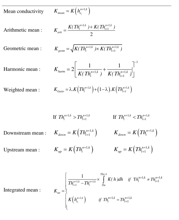
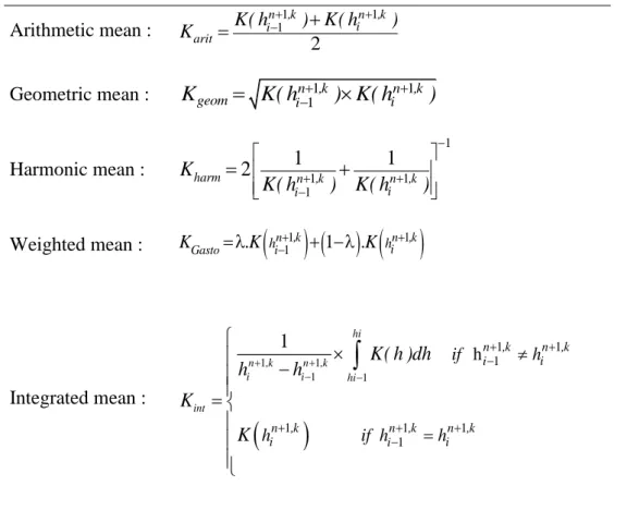
Table 1. Possible approximations of the MHFE equivalent conductivity 1
i
n ,k e
K for the
mesh ei between nodes i and i+1.
Mean conductivity Kmean K h
eni 1,k
Arithmetic mean : 1 1 1 2 in ,k in ,k arit K( Th ) K( Th ) K Geometric mean : 1 1 1 n ,k n ,k geom i i K K(Th ) K(Th ) Harmonic mean : 1 1 1 1 1 1 2 harm n ,k n ,k i i K K( Th ) K( Th ) Weighted mean :
1
1
11
n ,k n ,k Gasto i i K .K Th .K Th If Thin1,k Thin11,k If Thin1,k Thin11,k Downstream mean :
11
n ,k down i K K Th Kdown K Th
in1,k
Upstream mean : Kup K Th
in1,k
Kup K Th
in11,k
Integrated mean :
1 1 1 1 1 1 1 1 1 1 1 T 1
i Thi n ,k n ,k i i Thi int n ,k e n ,k n ,k i i n ,k n ,k i i if h Th if Th Th K( h )dh Th Th K K hn refers to the known time level (solution is assumed to be known at time n and unknown at
Table 2. Possible approximations of the FD interblock conductivities Kin1 21/,k. Arithmetic mean : 1 1 1 2 in ,k in ,k arit K( h ) K( h ) K
Geometric mean : Kgeom K( hin11,k ) K( h in1,k)
Harmonic mean : 1 1 1 1 1 1 2 harm n ,k n ,k i i K K( h ) K( h ) Weighted mean :
n ,k11
1
n ,k1 i Gasto hi h K .K .K Integrated mean :
1 1 1 1 1 1 1 1 1 1 1 h 1 hi n ,k n ,k i i hi int n ,k n ,k i i n ,k n ,k n ,k i i i if h h if h h K( h )dh h h K K
i refers to the known time level (solution is assumed to be known at time n and unknown at time n+1) and k to the nonlinear iteration level.
Table 3. Soil hydraulic parameters used for the two test cases in this study.
Variable Medium A Medium B Medium C
Material and/or Reference Berino loamy fine sand Glendale clay loam Celia et al. (1990) Hills et al. (1989)
r (-) 0.102 0.0286 0.106 s (-) 0.368 0.3658 0.4686 (cm-1) 0.0335 0.028 0.0104 n (-) 2 2.239 1.3954 Ks (cm.s-1) 9.22 10 3 6.26 10 3 1.52 10 4 Ss (cm-1) 8 1.0 10 1.0 10 8 1.0 10 8