A comparison of bootstrap approaches for estimating uncertainty of parameters in linear mixed-effects models.

HAL Id: inserm-00881820

https://www.hal.inserm.fr/inserm-00881820

HAL is a multi-disciplinary open access

archive for the deposit and dissemination of sci-entific research documents, whether they are pub-lished or not. The documents may come from teaching and research institutions in France or abroad, or from public or private research centers.

L’archive ouverte pluridisciplinaire HAL, est destinée au dépôt et à la diffusion de documents scientifiques de niveau recherche, publiés ou non, émanant des établissements d’enseignement et de recherche français ou étrangers, des laboratoires publics ou privés.

uncertainty of parameters in linear mixed-effects models.

Hoai-Thu Thai, France Mentré, Nicholas Holford, Christine Veyrat-Follet,

Emmanuelle Comets

To cite this version:

Hoai-Thu Thai, France Mentré, Nicholas Holford, Christine Veyrat-Follet, Emmanuelle Comets. A comparison of bootstrap approaches for estimating uncertainty of parameters in linear mixed-effects models.. Pharmaceutical Statistics, Wiley, 2013, 12 (3), pp.129-40. �10.1002/pst.1561�. �inserm-00881820�

estimating uncertainty of parameters in linear

mixed-effects models

Hoai-Thu Thai

, France Mentré

, Nicholas H.G. Holford

Christine Veyrat-Follet

, Emmanuelle Comets

A version of thenonparametric bootstrap, which resamples the entire subjects from original

data, called the case bootstrap, has been increasingly used for estimating uncertainty of pa-rameters in mixed-effects models. It is usually applied in order to get more robust estimates of the parameters and more realistic confidence intervals. Alternative bootstrap methods, such as residual bootstrap and parametric bootstrap which resample both random effects and resid-uals, have been proposed to better take into account the hierarchical structure of multi-level and longitudinal data. However, few studieshave been done to compare these different ap-proaches. In this study, we used simulation to evaluate bootstrap methods proposed for linear mixed-effect models. We also compared the results obtained by maximum likelihood (ML)

and restricted maximum likelihood (REML).Our simulation studies evidenced the good

per-formance of the case bootstrap as well as the bootstraps of both random effects and residuals. On the other hand, the bootstrap methods which resample only the residuals and the boot-straps combining case and residuals performed poorly. REML and ML provided similar bootstrap estimates of uncertainty, but there was slightly more bias and poorer coverage rate

for variance parameters with ML in the sparse design. We applied the proposed methods

to a real dataset from a study investigating the natural evolution of Parkinson’s disease and were able to confirm the methods provide plausible estimates of uncertainty.Given that most real-life datasets tend to exhibit heterogeneity in sampling schedules, the residual bootstraps

would be expected to perform better than the case bootstrap.

KEYWORDS: bootstrap; longitudinal data; Parkinson’s disease; linear mixed-effects models; R.

∗_{Correspondence to: Hoai-Thu Thai, UMR738 INSERM, University Paris Diderot, 75018 Paris, France;}

E-mail: hoai-thu.thai@inserm.fr

1_{INSERM, UMR 738, F-75018 Paris, France; Univ Paris Diderot, Sorbonne Paris Cité, UMR 738, F-75018}

Paris, France

2_{Department of Pharmacology and Clinical Pharmacology, University of Auckland, Auckland, New Zealand} 3_{Drug Disposition Department, Sanofi, Paris, France}

1

INTRODUCTION

Mixed-effects models are commonly used to analyze longitudinal data which consist of re-peated measures from individuals through time [1]. They play an important role in medical research, particularly in clinical trials. These models incorporate the fixed effects, which are parameters representing effects in the entire population, and random effects, which are associated with individuals sampled from a population [2]. The parameters of a model are estimated by maximum likelihood (ML) or restricted maximum likelihood (REML) method. In linear mixed-effects models, REML is often preferred to ML estimation because it takes into account the loss of the degrees of freedom involved in estimating the fixed effects,

re-sulting in unbiased estimates of variance components in many situations [2, 3].

The standard errors (SE) ofparameter estimatesare obtained asymptotically from the in-verse of the Fisher information matrix [2, 3]. The above estimates of SE might be biased when the asymptotic approximation is incorrect, for example when the sample-size is small. Sometimes, they can not be obtained when the model is complex or the design is too sparse. Bootstrap methods represent an alternative approach for estimating the SE of parameters, as well as to provide a confidence interval without assuming it is symmetrical. It was first introduced by Efron (1979) for independent and identically distributed (iid) observations. The principal idea of bootstrap is to resample the observed data repeatedly to create datasets similar to the original dataset, then fit them to construct the distribution of an estimator or a statistic of interest [4, 5]. Four main bootstrap approaches have been proposed for simple linear regression: case bootstrap, residual bootstrap, parametric bootstrap and wild bootstrap [6, 7, 8, 9]. The case bootstrap is the most simple and intuitive form which consists in resam-pling the entire vector of observations with replacement. The residual bootstrap resamples the residuals after model fitting. The parametric bootstrap adopts the principle of residual bootstrap but, instead of directly resampling observed residuals, we simulate the residuals

fromthe estimated distribution, e.g. the normal distribution,whose parameters are estimated

usingthe original data. The wild bootstrap consists in resampling the residuals from an

ex-ternal distribution satisfying certain specifications.

The main concern when bootstrapping is how to generate a bootstrap distribution close to the true distribution of the original sample. To do that, the bootstrap resampling should

ap-propriately mimicthe "true" data generating process (DGP) that produced the "true" dataset

[10, 11, 12]. In the context of repeated measurement data and mixed-effects modeling, the bootstrap should therefore respect the true DGP with the repeated measures within a subject and handle two levels of variability: between-subject variability and residual variability. The classical bootstrap methods developed in simple linear regression should be modified to take into account the characteristics of mixed-effects models [13]. Resampling random effects may be coupled with resampling residuals [10, 13, 14, 15]. The case bootstrap can be com-bined with the residual bootstrap [8]. The performance of these approaches are, however, not well studied.

In this paper, we extend different bootstrap approaches which can be applied to linear mixed-effects models settings. The detail of bootstrap methods are described in Section 2. The simulation settings are described in Section 3. The results of the simulation studies and the application of the bootstraps to real data collected in a study in Parkinson’s disease are described in Section 4. The discussion of the study is given in Section 5.

2

METHODS

2.1

Statistical models

Let Y be the response variable. N denotes the number of subjects. Let yij denote the ob-servation j of Y in subject i, while yi = (yi1, yi2, ..., yini)′ regroups the (ni × 1) vector of measurements in this subject. Let ntot = ∑N_i=1ni denote the total number of observations. We use the following linear mixed-effects model (LMEM) [16]:

     yi = Xiβ+ Ziηi+ ϵi η_i ∼ N (0, Ω) ϵi ∼ N (0, σ2Ini) (1) where Xi and Zi are (ni × p) and (ni × q) design matrices, β is the (p × 1) vector con-taining the fixed effects, η_i is the (q × 1) vector containing the random effects, and ϵi is the (ni× 1) vector of residual components. Ω is the general (q × q) covariance matrix with (i,j) element ωij = ωji andσ2Ini is the (ni× ni) covariance matrix for residual errors in subject i

where σ2_{is the error variance and I}

ni is the (ni× ni) identity matrix. The random effects ηi

are assumed to be normally distributed with mean 0 and covariance matrix Ω and the residual errors ϵi are assumed to be normally distributed with mean zero and variance σ2Ini. The ran-dom effects η_iand the residual errors ϵiare assumed to be independent for different subjects and to be independent of each other for the same subject.

Conditional on the random effects η_i, the response Yiin subject i is normally distributed with mean vector Xiβ+ Ziηi and with covariance matrix σ2Ini.

2.2

Estimation methods

The parameters of linear mixed-effects models can be estimated in the framework of imum likelihood by two general methods: maximum likelihood (ML) or restricted max-imum likelihood (REML). Let α denote the vector of all variance components of Vi = ZiΩ(Zi)′+ Σi, it means α consists of the q(q + 1)/2 different elements in Ω (or q elements if Ω is diagonal) and of all parameters in Σi. Let θ = (β′, α′)′ be the (s × 1) vector of all pa-rameters in the marginal model for Yi. The parameterestimatesare obtained by maximizing the marginal likelihood function with respect to θ.The ML likelihood function is defined as:

LM L(θ) = N ∏ i=1 { (2π)−ni/2 |Vi|− 1 2 × exp ( −1 2(yi− Xiβ) ′_V−1 i (yi− Xiβ) )} (2)

The REML likelihood function is derived from LM L(θ) to correct the loss of the degrees

of freedom involved in estimating the fixed effects: LREM L(θ) =    N ∑ i=1 X′ iV−1i Xi   − 1 2 LM L(θ) (3)

In this study, we used REML as the estimation method. However, we also compared the results of REML with those of ML and presented them in Appendix (available online as Supplementary Material).

When α is known, the maximum likelihood estimator (MLE) of β, obtained from maxi-mizing LM L(θ), conditional on α, is given by:

ˆ β(α) = ( _N ∑ i=1 X′ iVi−1Xi )−1 _N ∑ i=1 X′ iVi−1yi (4)

When α is unknown, but an estimate ˆα is available, we can set Vi = ˆVi and estimate β by using equation 4.

Estimates of the η_i can be obtained as the mean of the posterior distribution of η_i (empir-ical Bayes estimates, EBEs):

ˆ

η_i(θ) = E[ηi | yi] = ∫

η_if (ηi | yi)dηi = ΩZi′Vi−1(yi − Xiβ) (5) The MLE ˆθ of θ is asymptotically normally distributed with mean θ and asymptotic co-variance matrix given by the inverse of the Fisher information matrix MF. The asymptotic SE of parameters are then estimated as the square root of the diagonal element of the estimated covariance matrix.

2.3

Bootstrap methods

The principle of the bootstrap is to repeatedly generate pseudo-samples distributed according to the same distribution as the original sample. The unknown original distribution may be replaced by theempirical distribution of the sample, which is known asthe nonparametric bootstrap [17]. The bootstrap exists in another version called the parametric bootstrap [7, 9]. In this version, the underlying distribution F is estimated from the data by a parametric model, for instance a normal distribution and bootstrap samples are generated by simulating within

this distribution rather than from the empirical distribution as performed in the nonparamet-ric version. The resampling can be done with an independent distribution; this procedure is called external bootstrap or wild bootstrap. This approach was proposed by Wu to deal with heteroscedasticity [18]. We have chosen to deal with the simpler case of homoscedasticity and therefore have not investigated the wild bootstrap.

Let B be the number of bootstrap samples to be drawn from the original dataset, a general bootstrap algorithm is:

1. Generate a bootstrap sample by resampling from the data and/or from the estimated model

2. Obtain the estimates for all parameters of the model for the bootstrap sample

3. Repeat steps 1-2 B times to obtain the bootstrap distribution of parameter estimates and then compute mean, standard deviation, and 95% confidence interval of this distribu-tion

Let ˆθ∗

b be the parameter estimated for the bth bootstrap sample. Given a data set, the

expected value of the bootstrap estimator over the bootstrap distributionis calculated as the

average of the parameter estimates from the B bootstrap samples: ˆ θB = 1 B B ∑ b=1 (ˆθ∗ b) (6)

The bootstrap standard error is obtained as the sample standard deviation of the ˆθ∗ b: c SEB = v u u t 1 B − 1 B ∑ b=1 (ˆθ∗ b − ˆθB)2 (7)

A 95% bootstrap confidence interval can be constructed by calculating the 2.5th _and 97.5th_{percentile of bootstrap distribution:}

ˆ θ∗

(α·B) ≤ θ ≤ ˆθ((1−α)·B)∗ (8)

where α=0.025. An alternative approach is to use a normal approximation to construct a bootstrap confidence interval, using the estimated cSEB:

ˆ

θB− cSEB· z1−α/2 ≤ θ ≤ ˆθB+ cSEB· z1−α/2 (9) z1−α/2 denotes the 1 − α/2 quantile of the standard normal distribution, equal to 1.96 with α =0.05. However, it is preferable to use the bootstrap percentile confidence interval when bootstrapping[7, 19].

The detailed algorithms of bootstrap methods to obtain a bootstrap sample (bootstrap gen-erating process) are presented below in two separated groups: nonparametric and parametric bootstrap methods.

2.3.1 Nonparametric bootstrap

Nonparametric case bootstrap (Bcase,none). This method consists of resampling with replace-ment the entire subjects, that is the joint vector of design variables and corresponding re-sponses (Xi, Zi, yi) from the original data before modeling. It is also called the paired bootstrap. This procedure omits the second step of resampling the observations inside each subject. However, it is the most obvious way to do bootstrapping and makes no assumptions on the model.

Nonparametric case bootstrap coupled with global/individual residual bootstrap(Bcase,GR or Bcase,IR). This method resamples first the entire subjects with replacement. The individ-ual residindivid-uals are then resampled with replacement globally from the residindivid-ual distribution of the original simulated dataset or individually from the residual distribution of new subjects obtained after bootstrapping in the first step. The bootstrap sample is obtained as follows:

1. Fit the model to the data then calculate the residuals ˆϵi = yi− Xiβˆ − Ziηˆi

2. Draw N entire subjects {(X∗

i, Z∗i, yi∗)} with replacement from {(Xi, Zi, yi)} in the

original data and keep their predictions from model fitting X∗

iβˆ + Z∗iηˆ∗i and their

cor-responding residuals ˆϵ∗

i = y∗i − X∗iβˆ − Z∗iηˆ∗i. The new subject has n∗i observations.

3. Draw the residuals with replacement globally from all residuals of the original data or individually from each new subject

(a) Global residual resampling: draw a sample {ϵ∗_}={ˆϵ

i∗_j∗} of size n∗_tot = ∑N_i=1n∗_i

with replacement globally from {ˆϵ} = {ˆϵij}i=1,..,N ;j=1,..,ni by assigning an equal

probability 1

ntot to each value of the ntotresiduals (note that, n

∗

totmay be different

with ntot)

(b) Individual residual resampling: draw individually N samples{ϵ∗

i}={ˆϵ∗ij∗} of size

n∗

i with replacement from ˆϵ∗i = {ˆϵ∗ij}j=1,..,n∗

i by assigning an equal probability

1 n∗

i

to each residual of new subject i

4. Generate the bootstrap responses y∗

i = X∗iβˆ + Z∗iη∗i + ϵ∗i

Here, and in the following, we note the vector of estimated residuals for all subjects as ˆϵ = {ˆϵij}i=1,..,N ;j=1,..,ni and the vector of estimated residuals in subject i as ˆϵi = {ˆϵij}j=1,..,ni. Nonparametric random effects bootstrap coupled with global/individual residual boot-strap (Bη,GR or Bη,IR). This method consists of resampling with replacement the random effects obtained after model fitting, as well as the residuals globally or individually. The bootstrap sample is obtained as follows:

1. Fit the model to the data then estimate the random effects ˆη_i and the residuals ˆϵi = yi− Xiβˆ − Ziηˆi

2. Draw a sample {η∗

i} of size N with replacement from { ˆηi} by assigning an equal

probability 1

3. Draw a sample {ϵ∗_}={ˆϵ

i∗_j∗}of size n_tot with replacement globally from {ˆϵ} or draw

individually N samples {ϵ∗

i}={ˆϵij∗}of size n_i with replacement from {ˆϵ_i} 4. Generate the bootstrap responses y∗

i = Xiβˆ + Ziη∗i + ϵ∗i

Nonparametric global/individual residual bootstrap (Bnone,GR / Bnone,IR). For the sake of completeness, we also implemented a bootstrap where only residual variability is resam-pled. These procedures do not resample the between-subject variability (which remains in the model through the estimated random effects ˆη_i). The bootstrap sample is obtained as follows:

1. Fit the model to the data then calculate the residuals ˆϵi = yi− Xiβˆ − Ziηˆi 2. Draw a sample {ϵ∗_}={ˆϵ

i∗_j∗}of size n_tot with replacement globally from {ˆϵ} or draw

individually N samples {ϵ∗

i}={ˆϵij∗}of size ni with replacement from {ˆϵi} 3. Generate the bootstrap responses y∗

i = Xiβˆ + Ziηˆi+ ϵ∗i

The nonparametric bootstrap methods that resample the random effects or the residuals depend on the structural model to calculate the raw random effects or residuals. However, they do not require particular assumptions on their distributions.

2.3.2 Parametric bootstrap

The parametric bootstrap requires the strongest assumptions as it depends both on the model and the distributions of parameters and errors.

Case bootstrap coupled with parametric residual bootstrap(Bcase,PR). Similar to Bcase,GR, this methods resamples firstly the subjects and then resamples the residuals by simulating from the estimated distribution. This methodcombines elements of both thenonparametric bootstrap (case bootstrap in the first step) and the parametric bootstrap (residual bootstrap in the second step). However, to simplify the classification, we keep it in the group of parametric bootstraps. The bootstrap sample is obtained as follows:

1. Fit the model to the data

2. Draw N entire subjects {(X∗

i, Z∗i, yi∗)} with replacement from {(Xi, Zi, yi)} in the

original dataand keep their predictions from model fitting X∗

iβˆ + Z∗iηˆ∗i 3. Draw N samples {ϵ∗

i} of size n∗i from a normal distribution with mean zero and

co-variance matrix ˆσ2_I ni

4. Generate the bootstrap responses y∗

i = X∗iβˆ + Z∗iηˆi+ ϵ∗i

Parametric random effects bootstrap coupled with residual bootstrap (BPη,PR). This methods resamples both random effects and residuals by simulating from estimated distri-bution after model fitting. The bootstrap sample is obtained as follows:

2. Draw a sample {η∗

i}of size N from a multivariate normal distribution with mean zero

and covariance matrix ˆΩ 3. Draw N samples {ϵ∗

i}of size nifrom a normal distribution with mean zero and

covari-ance matrix ˆσ2_I ni

4. Generate the bootstrap responses y∗

i = Xiβˆ + Ziη∗i + ϵ∗i

Parametric residual bootstrap (Bnone,PR). Again for exhaustiveness, we implemented a bootstrap which resamples only the residuals by simulating from the estimated distribution after model fitting. Similar to Bnone,GR or Bnone,IR , this procedure omits the first step of resampling the between-subject variability. The bootstrap sample is obtained as follows:

1. Fit the model to the data 2. Draw N samples {ϵ∗

i}of size nifrom a normal distribution with mean zero and

covari-ance matrix ˆσ2_I ni

3. Generate the bootstrap responses y∗

i = Xiβˆ + Ziηˆi+ ϵ∗i 2.3.3 Transformation of random effects and residuals

Previous results in the literature show that the nonparametric bootstrap of the raw residu-als obtained by model fitting usually yield downwardly biased variance parameter estimates [7, 8, 20]. In ordinary linear models, this underestimation is due to the difference between estimated and empirical variance of residuals [21]. That’s why it is advisable to rescale the residuals so that they have the correct variance. Efron suggested to multiply centered raw residuals with the factor √(n − p)/n where p is the number of parameters and n is the number of observations [22]. For the same reason, Davison et al proposed to use the factor √

1/(1 − hi) where hi is the ith diagonal element of the hat matrix which maps the vectors of observed values to the vector of fitted values [7]. In mixed-effects models, this is because the raw variance-covariance matrix is different from the maximum likelihood estimate, as the raw random effects or residuals are "shrunk" towards 0 [20]. Carpenter et al proposed to take this into account by centering the random effects and residuals to resample from a distribution with mean zero and multiplying them by the ratio between their corresponding estimated and empirical variance-covariance matrices to account for the variance underestimation [20, 23]. These corrections were used in our study.

Transforming random effects. The transformation of random effects was carried out in the following steps:

1. Center the raw estimated random effects: ˜η_i = ˆη_i− ¯η_i

2. Calculate the ratio between the estimated and empirical variance-covariance matrix (Aη). Let ˆΩ be the model estimated variance-covariance matrix of random effects and Ωemp denote the empirical variance-covariance matrix of the centered random effects

˜

η_i. The ratio matrix Aη is formed by using the Cholesky factors Lest and Lemp, which are the lower triangular matrix of the Cholesky decomposition of ˆΩ and Ωemp, respec-tively: Aη = (Lest· L−1emp)

3. Transform the centered random effects using the ratio Aη: ˆη ′

i = ˜ηi× Aη

Transforming residuals. The transformation of residuals was carried outglobally for all

residualsin the following steps:

1. Center the raw estimated residuals: ˜ϵij = ˆϵij − ¯ϵij

2. Calculate the ratio between the estimated and empirical variance-covariance matrix (Aσ). Let ˆΣ be the model estimated variance-covariance matrix for residuals, which is assumed to be equal to ˆσ2_I

niand Σempdenote the empirical variance-covariance matrix of centered residual ˜ϵij. Because the residuals are assumed to be uncorrelated and to have equal variance, the ratio matrix Aσ is then simply the ratio between the square root of the model estimated residual variance ˆσ2 _{and the empirical standard deviation} of the centered residuals, respectively: Aσ = ˆσ/sd(˜ϵij).

3. Transform the centered residuals using the ratio Aσ: ˆϵ ′

ij = ˜ϵij × Aσ

3

SIMULATION STUDIES

3.1

Motivating example

The motivating example for bootstrap evaluation was a disease progression model inspired from the model of Parkinson’s disease developed by Holford et al [24]. In that study, the subjects were initially randomized to treatment with placebo, with deprenyl, with tocopherol or with both and, when clinical disability required, received one or more dopaminergic agents (levodopa, bromocriptine or pergolide). The aim was to study the influence of various drugs on the changes in UPDRS (Unified Parkinson’s Disease Rating Scale) over time. Several components describing the disease progression and the effect of treatment were developed. However, in this study, we are only interested in the linear part of the model, describing the

natural evolution of Parkinson’s disease using a random intercept and slope model as:

yij = S0+ α · tij + ηS0_i+ ηαi· tij+ ϵij (10)

where yij is the UPDRS score (u) representing the state of disease at time tij which was

considered to be continuous, S0 (u) is the expected score at randomization, α (u/year) is the

progression rate, ηS0_i (u/year) and ηαi (u/year) are the random effects of S0 and α,

respec-tively and ϵij is the residual errors. In the formulation of equation (1), the design matrix

Xi = Zifor subject i is a two-column matrix with a first column of 1s and a second column

containing the nitimes tij for subject i.

For our simulations, we used the subset of patients who remained in the placebo group over the first 2 years.The UPDRS scores were measured at randomization and at regular

(un-scheduled) visits up to 2 years after entry to the study. This subset contains 109 subjects with

an average of 6 observations per subject and a total of 822 observations. Figure1 describes the evolution of UPDRS score over a two-year period.

In the paper of Holford et al, the baseline S0was assumed to be log-normally distributed, and the progression rate α was assumed to be normally distributed [24]. The variance of the random effects and the correlation ρ between S0 and α was estimated. The residual unexplained variability was described by an additive model error with constant variance σ2_. In the present study, both S0 and α were assumed to be normally distributed. We estimated the parameters of the real dataset byML, the same estimation method as used in the original publication [24], using the lme function in R. The detail of parameter estimates is given in section 4.2.

3.2

Simulation settings

Our simulations were inspired from the original design described above using estimates from the real dataset.

Three designs were planned to evaluate the performance of bootstrap. For each design, the sampling times were similar for all subjects.

Rich design. We simulated N=100 subjects with n=7observationsper subject at 0, 0.17, 0.33, 0.5, 1, 1.5, 2 years after being entered in the study.

Sparse design. We simulated N=30 subjects with n=3observationsper subject at 0, 0.17, 2 years after being entered in the study. This design is sparse with respect to estimation of variance parameters, including only 90 observations in total.

Large error design. We simulated N=100 subjects with n=7observations per subject at 0, 0.17, 0.33, 0.5, 1, 1.5, 2 years after being entered in the study. In this design, we mod-ified the level of variability. The variability for random effects ηS0 and ηα were changed to

ωS0=11.09 and ωα=6.98 respectively (equivalent to 50% of the corresponding fixed-effects),

and the standard deviation for the residual error was changed to σ=17.5. We also removed the correlation ρ between S0and α in this design because convergence was obtained for only 78.3% simulated datasets with the presence of this correlation.

For each design, we simulated K=1000 replications.

3.3

Software

The lme function in the nlme library in R was used to fit the data using REML as the esti-mation method. ML was also used to compare with the results of REML. For both methods, we fitted datasets with the initial values of variance parameters generated by the optimisation procedure implemented in the lme function [25]. All the analysis and figures were done with R.

3.4

Evaluation of bootstrap methods

Table 1 presents all the bootstrap methods that we implemented and evaluated. The resam-pling of the between-subject variability (BSV) can be done by resamresam-pling subjects or random effects. The resampling of the residual variability (RUV) can be done by resampling of resid-uals obtained from all subjects, called global residresid-uals or resampling of residresid-uals within each subject, called individual residuals. In order to compare the performance of these bootstraps to that of classical bootstraps, the residual bootstrap, which resamples only the RUV, and the case bootstrap where the whole vector of observations, including both the BSV and RUV, is resampled were also evaluated in our study. The bootstrap methods were classified as nonparametric and parametric methods. For the parametric approach, there is no difference between the global and the individual residual resampling because it is performed by sim-ulation from the estimated distributions. In total, we had 7 nonparametric methods and 3 parametric methods.

We drew B= 1000 bootstrap samples for each replication of simulated data and for each bootstrap method. The parameters were estimated byREMLmethod using the lme function in R. For each method, we therefore performed 1 million fits (1000 simulated datasets × 1000 bootstrap datasets). If the convergence was not obtained, the NA was recorded in the table of parameter estimates and excluded for further calculation.

For the kth _{simulated dataset and for a given bootstrap method, we computed the} boot-strap parameter estimate ˆθk

B as in equation (5), using 1000 bootstrap samples, as well as the boostrap SE and CI, for each parameter θ.The relative bias (RBias) of bootstrap estimate was

obtained by comparing the bootstrap estimate ˆθk

B and the asymptotic estimate ˆθkas follows:

RBias(ˆθB) = 1 K K ∑ k=1 ( ˆθk B− ˆθk ˆ θk × 100) (11)

The average bootstrap SE was obtained by averaging the SE from equation (6) over the K=1000 datasets. The true SE is unknown, but we can get an empirical estimate as the standard deviation of the differences between the estimate of the parameter in the K datasets and the true value (θ0):

SEempirical(ˆθ) = v u u t 1 K − 1 K ∑ k=1 (ˆθk− θ0)2 (12)

The relative bias on bootstrap SE was then obtained by comparing the average bootstrap SE to this empirical SE:

RBias(SE(ˆθB)) = 1 K ∑K k=1SEB(ˆθBk) − SEempirical(ˆθ) SEempirical(ˆθ) × 100 (13)

The coverage rate of the 95% bootstrap confidence interval (CI) was defined as the per-centage of the K=1000 datasets in which the bootstrap CI contains the true value of the

parameter.

The bootstrap approaches were compared in terms of the Rbias on the bootstrap parame-ter estimates, the Rbias on SE, and the coverage rate of the 95% CI of all parameparame-ter estimates from one million bootstrap samples.

The performance of the bootstrap methods were also compared to the performance of the asymptotic method. It is worth noting that in the simulation studies, random variables were simulated according to normal distributions, which may have contributed to the good

performance of the asymptotic method.The relative bias of asymptotic estimate was obtained

by comparing the asymptotic estimate ˆθkand the true value θ0as follows: RBias(ˆθ) = 1 K K ∑ k=1 ( ˆθk− θ0 θ0 × 100) (14)

The relative bias of asymptotic SEs given by the software (obtained as the inverse of the Fisher information matrix) was defined in the same way as equation (13), but with respect to ˆ

θkin stead of ˆθBk. The coverage rate of the 95% asymptotic CI was defined as the percentage of datasets in which the asymptotic CI contains the true value of the parameter.

Theasymptoticand bootstrap parameters estimates and their SE were defined as unbiased

when relative bias was within ±5%, moderately biased (relative bias from ±5% to ±10%) or strongly biased (relative bias > ±10%). The coverage rate of the 95% CI was considered to be good (from 90% to 100%), low (from 80% to 90%) or poor(< 80%). A good bootstrap was defined as a method providing unbiased estimates for the parameters and their corresponding SE, and ensuring a good coverage rate of the 95% CI.

3.5

Application to real data

All the bootstrap methodswith good performanceevaluated in the simulations studies were applied to the real databy drawing B=1000 bootstrap samples for each method. The bootstrap parameter estimates and bootstrap SE were compared with each other and compared to the parameter estimates and their SEs obtained by the asymptotic approach.

4

RESULTS

4.1

Simulation studies

Examples of simulated data for each given design are illustrated in Figure 2. Our simulations gave some negative values for the observations because of the homoscedastic error model. These values were kept as is, since the purpose of the simulations was not to provide a real-istic simulation of the trial, but only to evaluate the bootstrap methods. For the same reason,

we did not take into account other real-life factors such as drop-outs or missingness.

We present firstly the results of REML. Complete results for all bootstrap methods as well as the asymptotic method in the 3 evaluated designs are reported in Table 2, for relative bias of the bootstrap estimates of parameters and their corresponding SEs, and Table 3, for

the coverage rate of the 95% CI. The correlation between S0 and α was not estimated in

the large error design for both simulated and bootstrap datasets to have better convergence

rate and to keep the same model which we simulated. The transformation of random effects

and residuals were done before resampling for the methods in which they were resampled nonparametrically. In the rich design, we found that the bootstrap methods which resample only the residuals (Bnone,GR ,Bnone,IR ,Bnone,PR) yielded higher bias for the correlation term

(>9.73%). The same was observed for the case bootstrap coupled with the residual

boot-straps (Bcase,GR, Bcase,IR, Bcase,PR). The case bootstrap and the bootstraps of both random effects and residuals (Bη,GR, Bη,IR, BPη,PR) showed essentially no bias for all parameters. In terms of SE estimation, these four bootstrap methods estimated correctly all the SEs, as the estimates were very close to empirical SEs, while the residual-alone bootstraps greatly underestimated the SEs of all parameters, except for that of σ. On the contrary, the SE of σ was overestimated by the Bcase,IR. The case bootstrap, coupled with global residual bootstrap (Bcase,GR) or parametric bootstrap (Bcase,PR), gave better estimates for SE of parameters than the residual-alone bootstraps, but they did not work as well as the case bootstrap and the boot-strap of random effects and residuals. In terms of coverage rate, the residual-alone bootboot-straps had very poor coverage rates for all parameters (< 0.6) except for the SE of σ, while the case bootstrap and the bootstraps of both random effects and residuals provided the good coverage rates (close to the nominal value of 0.95). According to our predefined criteria, four methods showed good performance: Bcase,none, Bη,GR, Bη,IR and BPη,PR. These methods remained the best methods for the sparse design and the large error design, with smaller relative bias for the parameter estimates and their SEs and better coverage rates. The simulation results also showed that the asymptotic approach provided good estimates for parameters and SEs as well as good coverage rates as do the bootstrap candidates. In this simple setting, the convergence rate was high: nearly all runs on the simulated datasets converged (respectively 100%, 99.8% and 99.9% for the rich, sparse and large error designs). Convergence was also close to 100% when applied to the bootstrap samples in the rich (100%) and large error (99.9%) design while for the sparse design, convergence rates were slightly lower and more dependent on the bootstrap method, going from around90.2%for the bootstraps combining case and residuals,

to96.7%for the case bootstrap or the bootstraps of both random effects and residuals.

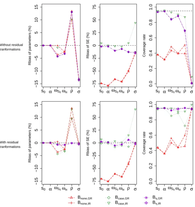
In this study, we also evaluated the influence of transformation of random effects and residuals using the ratio between the estimated and empirical variance-covariance matrices. Non-transformed and transformed resampling were compared for all non-parametric boot-strap methods except for the Bcase,none where no transformation was needed. The results of this transformation in the rich design are presented in Figure 3. We found that these cor-rections improved significantly the estimate of σ, its SE as well as the coverage rate for all applied methods. However, they only improved the estimates and the coverage rates of other

variance parameters for Bη,GRand Bη,IR.

The results for the bootstrap candidates in the different evaluated designs, providing a more contrasted evaluation of their performance were shown in Figure S1 in Appendix. All the bootstrap candidates provided good parameter estimates in all evaluated designs with the

relative bias within ± 5%, except for a higher bias on σ (-6.50%) observed for the Bη,IR in

the sparse design. The relative bias for the variance estimates were higher for the sparse and the large error designs compared to those of the rich design, while the relative bias of the

fixed effects remained very small (< 0.1%). All the bootstrap candidates estimated correctly

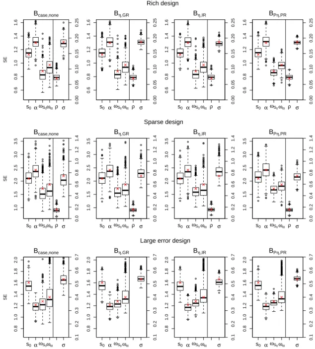
the SE of parameters, with relative biases ranging from -5% to 5%, observed in both rich and large error designs. They estimated less correctly the SE of variance parameters in the sparse design with relative biases ranging from -10% to 10%, especially for the case bootstrap. The boxplots of the SEs of all parameter estimates obtained by the bootstrap candidates in all evaluated designs are shown in Figure S2 in Appendix. The range of bootstrap standard er-rors across the K=1000 replications did not show any practically relevant differences across

the bootstrap methods, with the exception of SE of σ in the sparse design. A good coverage

rate was obtained for all parameters in the rich design setting, as well as the design with large error; the one exception is a low coverage rate for σ observed for Bη,IR in the design with large error. In the sparse design, the bootstrap candidates provided lower coverage rate for variance parameters. Across the different designs, the BPη,PRworked slightly better than the Bcase,noneand the Bη,GRperformed better than the Bη,IR.

In order to understand whether the estimation method influences the performance of the bootstrap methods, we compared the results of ML with those of REML. All the results of ML are given in Appendix with Table S1 and Table S2. The difference between ML and REML in relative bias of parameter estimates and their SEs and coverage rate for all boot-strap methods and the asymptotic method in three evaluated designs are shown in Figure S3 in Appendix. There was no difference in estimation of fixed effects and σ between two

methods. However, the variance parameters (ωS0 and ωα) given by ML were slightly less

well estimated compared to those of REML with increase of 0.5 to 2% in relative bias and had lower coverage rate in all evaluated designs. The difference between ML and REML in estimation of variance parameters was more apparent in the sparse design, resulting in bigger difference in their coverage rates (2 to 5%) observed for all bootstrap methods. In terms of SE estimation, ML and REML provided similar estimates, except for a small difference in relative bias (<2%) in the sparse design. Based on our criteria about relative bias, REML was better than ML by providing unbiased estimates for almost parameters obtained by four bootstrap candidates. REML also improved the coverage rate of variance parameters in the sparse design while it provided similar estimates of SEs compared to ML.

4.2

Application to real data

The asymptotic parameter estimates by ML and their SEs for the real dataset were given in the first row of Table 4;these were taken as the true parameter values used in the simulation

study reported above. The parameter estimatesby REMLand the SEs of all parameters

ob-tained by the asymptotic method and the 4 bootstrap candidates for the real dataset are also shown in Table 4. They provided similar values for both fixed-effect and variance parameters which were also close to the asymptotic estimates. However, there were some differences

for the estimation of SE of α, ωα and σ between the bootstrap methods. The Bcase,none yield

the highest SE for these parameters while the BPη,PRand the asymptotic estimates were very

similar, which were both different from the remaining bootstrap methods. This finding was not observed in the simulation study, where balanced designs with the same number of obser-vations per subject were used and the residuals were normally distributed. The distribution of the empirical residuals in the real dataset was investigated and a non normal distribution was confirmed by the Shapiro-Wilk normality test. The similar results of ML for the real data are also presented in Table S3 in Appendix.

In order to investigate the effect of the unbalance in the design, we stratified the case bootstrap based on the number of observations per subject (nobs). The real dataset was di-vided into 3 groups before bootstrapping: group 1 (N=40 subjects with nobs <= 5), group 2 (N=38 subjects with nobs > 5 and <=10) and group 3 (N=31 subjects with nobs > 10). The bootstrap samples were then built by sampling subjects within each group, keeping the same number of subjects from each group. The results obtained from this analysis are also given in Table 4. The case bootstrap with stratification Bstrat

case,none gave similar values for parameters as the case bootstrap and other bootstrap methods. In terms of SE of parameters, this method provided smaller values for SEs of α and ωαand reduced the difference on SE estimation of these parameters with other bootstrap methods, which may indicate that the case bootstrap is more sensitive to unbalanced designs; on the other hand, stratification hardly affected the SE of σ.

5

DISCUSSION

In this paper, we evaluated different bootstrap approaches for estimating standard errors and confidence intervals of parameters in linear mixed-effects models with homoscedastic error. The proposed bootstraps take into account two levels of variability in the longitudinal data: BSV and RUV. They were also compared to the residual bootstrap, which resamples only one level of variability, and to the case bootstrap where the whole vector of observations is resampled.

Our simulations showed that bootstrapping only residuals underestimated greatly the SEs of parameters, except for σ and provided poor coverage rates. This finding is to be expected because the large BSV for two parameters in the evaluated designs were not taken into

ac-count. On the contrary, the case bootstrap performed well as it provided non-biased parameter estimates and SEs as well as good coverage rates for all parameters. Moreover, according to Van der Leeden et al, it makes sense to resample only the individuals and collect the related observations from the original dataset when bootstrapping cases for the repeated measures data [14, 26]. Our results support the implication that the residual variability is somewhat taken into account in this method; resampling cases preserves both the BSV and the RUV. It is in agreement with the worse performance of combining residual bootstrap with case boot-strap, in which the RUV is considered already resampled.

Another important result of this study is the good performance of bootstrapping both ran-dom effects and residuals, either in a nonparametric or in a parametric way. They worked as well as the case bootstrap. The incorporation of random effects into the classical resid-ual bootstrap plays therefore a very important role for bootstrapping in mixed-effects models context, especially when the BSV is much higher than the RUV. This approach was proposed in various studies, such as for the resampling of multi-level data [14, 23], times series data [10] and more recently for longitudinal data [15]. It can be an alternative method to the case bootstrap when the model is correct (for nonparametric version) or both model and assump-tions on distribuassump-tions of parameters are correct (for parametric version). To our knowledge, there has not been any simulation study in the literature which compares this approach to the most commonly used method, the case bootstrap for mixed-effects models with longitudinal data.

Bootstrapping the raw random effects and residuals does not take into account variance underestimation, leading to shrinkage in the individual parameter estimates. To account for this issue, we employed the correction using the ratio between estimated and empirical variance-covariance matrix for the random effects and the residuals. It was shown to be an ap-propriate method for linear mixed-effects models because of the improvement of estimation for variance components. These ratios account for the degree of two shrinkages: η-shrinkage and ϵ-shrinkage, which quantify the amount of information in the individual data about the parameters [27, 28, 29]. When the data is not informative, the random effects and residuals are shrunk toward 0 and high degree of η-shrinkage and ϵ-shrinkage will be obtained. Sam-pling in the raw distribution will therefore underestimate the actual level of variability in the data, while correcting both empirical random effects and residuals for shrinkage restores this level. This idea of accounting for the difference between the estimated and empirical variance of residuals through an estimate of the shrinkage was proposed in bootstrapping ordinary lin-ear models [21], and was extended for the two levels of variability found in mixed models by Wang et al [23].

The performance of different bootstrap methods was evaluated under different conditions: the rich design in which all parameters can be well estimated, the sparse design in which the variance parameters are less well estimated and the large error design in which the RUV is as important as the BSV to see whether the residual bootstraps work better.The convergence was obtained for almost all bootstrap datasets (90% to 100%), which should not provide

substantial bias for estimating the uncertainty of parameters. The case bootstrap and three bootstrap methods where both random effects and residuals were resampled remained the best methods and selected as bootstrap candidates for linear mixed-effects models. The purpose of this work was not to determine which was the best method overall, but to eliminate boot-strap methods that do not perform well even with linear mixed-effects models. We did note that the global residual bootstrap was slightly better than individual residual bootstrap in the sparse and large error designs,especially in estimating σ; which is consistent with the non-correlated structure of residuals. In addition, the distribution of resampled residuals obtained by the global residual bootstrap was slightly closer to the original distribution of residuals. The parametric bootstrap performed best across three evaluated designs, but it requires the strongest assumptions (good prior knowledge about model structure and distributions of pa-rameters). If the model is misspecified and the assumptions of normality of random effects and residuals are not met, this method may not be robust. In practice, one of the main reasons for using bootstrap is the uncertainty of distribution assumption, the nonparametric bootstrap may therefore preferable to the parametric bootstrap in most applications [9].

We also investigated using ML instead of REML when performing the estimation step. The difference in performance was small with less than 5%, but there was slightly more bias with ML especially for the estimation of the variance parameters, which was most apparent in the sparse design where variances were less well estimated. This means that we may expect this to be true also for non-linear mixed effect models where ML is more often used than REML for parameter estimation, although this needs to be verified in the non-linear setting. This finding should be also explored further in other settings, since the superiority of REML over ML becomes more apparent as the number of fixed effect increases, especially when the number of subjects is limited [3].

The number of bootstrap replicates (B) depends on the estimation which we want to ob-tain. In simple regression models, B is recommended to be at least 100 for SE estimation and at least 1000 in the case of confidence interval estimation [30, 31]. In this simulation study, 1000 bootstrap replicates were thought to be large enough to obtain both bootstrap SE and bootstrap confidence interval for all bootstrap methods with linear mixed-effects

mod-els. Note that, in order to estimate directly the quantiles for 95% CI without interpolation,

B=999 should be used instead of 1000 in the future work [7]. In addition,further evaluation

on choosing the number of bootstrap will be studied, especially when bootstrapping on non-linear mixed-effects models is much time-consuming and less stable.

Although in the simulation studies, the performance of the case bootstrap was similar to that of the bootstrap methods resampling both random effects and residuals, when these methods were applied to the real dataset, the case bootstrap estimated a much larger SE for both α and its variability, and there was also smaller differences in the estimates of σ between the different bootstraps. We found a good agreement between the BPη,PRand the asymptotic method, which were both different from the remaining methods. The difference between

for-mer we sample in a normal distribution while the empirical residuals used for resampling in

Bη,GRwere in fact not normally distributed. The difference between Bcase,none and Bη,GRor

Bη,IRmight due to the unbalanced design of the real dataset in which patients have different

number of observations, a structure which is preserved by the residual-bootstraps but not by

the case bootstrap. Unbalanced designs, therefore, may be more challenging for the case

bootstrap than for other bootstrap methods [7, 32], and stratification has been proposed to handle such situations; for example when a study includes rich and sparse data it is recom-mended to resample from both groups to maintain a similar structure in the bootstrap samples [33]. In this study, we tried to apply the stratified case bootstrap to the real dataset. The strat-ification could explain a part of the difference between the case bootstrap and other bootstrap candidates by decreasing the SEs of α and ωαto the values closer to those obtained by other methods.

In conclusion, in this study, we found that the case bootstrap performs as well as the nonparametric/parametric bootstrap of random effects and residuals in linear mixed-effects models with balanced designs and homoscedastic error. However, the residual bootstraps always generate datasets with the same design as the original data and would be expected to perform better in situations where the design is not similar for every individual. This could be the explanation for the discrepancy between the bootstraps seen in the application to the real data from the Parkinson study. We now plan to compare these methods for nonlinear mixed-effects models, addressing the issues of heteroscedasticity, the nonlinearity of model, and exploring the influence of designs with stratified bootstrap.

Acknowledgements

The authors would like to thank the Parkinson Study Group for providing us the data from Parkinson’s study as well as IFR02 and Hervé Le Nagard for the use of the "centre de biomod-élisation". We also thank the reviewer for a careful review and insightful comments that helped us to improve this paper.

During this work, Hoai-Thu Thai was supported by a research grant from Drug Disposi-tion Department, Sanofi, Paris.

References

1. Fitzmaurice GM, Laird NM, Ware JH. Applied longitudinal analysis. John Wiley & Sons: New York, 2004.

2. Pinheiro JC, Bates DM. Mixed-effects models for S and S-plus. Springer: New York, 2000.

3. Verbeke G, Molenberghs G. Linear mixed models for longitudinal data. Springer: New York, 2000.

4. Efron B. Bootstrap methods: Another look at the jacknife. The Annals of Statistics 1979; 7(1):1–26.

5. Efron B, Tibshirani RJ. An introduction to the bootstrap. Chapman & Hall: New York, 1994.

6. Shao J, Tu D. The jacknife and bootstrap. Springer: New York, 1995.

7. Davison AC, Hinkley DV. Bootstrap methods and their application. Cambridge Univer-sity Press: Cambridge, 1997.

8. MacKinnon JB. Bootstrap methods in econometrics. The Economic Record 2006; 82(s1):S2–S18.

9. Wehrens R, Putter H, Buydens LMC. The bootstrap: a tutorial. Chemometrics and Intel-ligent Laboratory Systems2000; 54(1):35–52.

10. Ocana J, El Halimi R, Ruiz de Villa MC, Sanchez JA. Bootstrapping repeated measures data in a nonlinear mixed-models context. Mathematics Preprint Series 2005; 367:1–31. 11. Flachaire E. Bootstrapping heteroskedastic regression models: wild bootstrap vs. pairs

bootstrap. Computational Statistics and Data Analysis 2005; 49(2):361–376.

12. Halimi R. Nonlinear Mixed-effects Models and Bootstrap resampling: Analysis of Non-normal Repeated Measures in Biostatistical Practice. VDM Verlag Dr. MÃijller: Berlin, 2005.

13. Das S, Krishen A. Some bootstrap methods in nonlinear mixed-effect models. Journal of Statistical Planning and Inference1999; 75(2):237–245.

14. Van der Leeden R, Busing FMTA, Meijer E. Bootstrap methods for two-level models. Technical Report PRM 97-04, Leiden University, Department of Psychology, Leiden 1997.

15. Wu H, Zhang JT. The study of long-term hiv dynamics using semi-parametric non-linear mixed-effects models. Statistics in Medicine 2002; 21(23):3655–3675.

16. Laird NM, Ware JH. Random-effects models for longitudinal data. Biometrics 1982; 38(4):963–974.

17. Ette EI. Stability and performance of a population pharmacokinetic model. Journal of Clinical Pharmacology1997; 37(6):486–495.

18. Wu CFJ. Jacknife, bootstrap and other resampling methods in regression analysis. The Annals of Statistics1986; 14(4):1261–1295.

19. Carpenter J, Bithell J. Bootstrap confidence intervals: when, which, what? a practical guide for medical statisticians. Statistics in Medicine 2000; 19(9):1141–1164.

20. Carpenter JR, Goldstein H, Rasbash J. A novel bootstrap procedure for assessing the relationship between class size and achievement. Applied Statistics 2003; 52:431–443.

21. Moulton LH, Zeger SL. Bootstrapping generalized linear models. Computational Statis-tics and Data Analysis1991; 11(1):53–63.

22. Efron B. The jacknife, the bootstrap and other resampling plans. Society of Industrial and Applied Mathematics: Philadelphia, 1982.

23. Wang J, Carpenter JR, Kepler MA. Using SAS to conduct nonparametric residual boot-strap multilevel modeling with a small number of groups. Computer Methods and Pro-grams in Biomedicine2006; 82(2):130–143.

24. Holford NHG, Chan PLS, Nutt JG, Kieburtz K, Shoulson I, Parkinson Study Group. Dis-ease progression and pharmacodynamics in Parkinson disDis-ease–evidence for functional protection with levodopa and other treatments. Journal of Pharmacokinetics and Phar-macodynamics2006; 33(3):281–311.

25. Bates DM, Pinheiro JC. Computational methods for multilevel models. Technical mem-orandum bl0112140-980226-01tm, Bell Labs, Lucent Technologies, Murray Hill, NJ 1998.

26. De Leeuw J, Meijer E. Handbook of multilevel analysis, chap. Resamling multilevel models. Springer: New York, 2007.

27. Ette EI, Williams PJ. Pharmacometrics: the science of quantitative pharmacology. Wiley-Blackwell: New Jersey, 2007.

28. Karlsson MO, Savic RM. Diagnosing model diagnostics. Clinical Pharmacology and Therapeutics2007; 82(1):17–20.

29. Savic RM, Karlsson MO. Importance of shrinkage in empirical bayes estimates for diag-nostics: problems and solutions. The AAPS journal 2009; 11(3):558–569.

30. Chernick MR. Bootstrap methods: A guide for practitionners and researchers. Second edn., John Wiley & Sons: New Jersey, 2007.

31. Bonate PL. Pharmacokinetic-pharmacodynamic modeling and simulation. Second edn., Springer: New-York, 2011.

32. Davison AC, Kuonen D. An introduction to the bootstrap with applications in R. Statis-ticial Computing and Statistical Graphics Newsletter2002; 13(1):6–11.

33. Lindbom L, Pihlgren P, Jonsson EN. PsN-Toolkit–A collection of computer intensive statistical methods for non-linear mixed effect modeling using NONMEM. Computer Methods and Programs in Biomedicine2005; 79(3):241–257.

Table 1 – Bootstrap methods that can be applied in mixed-effects models Variability related to subject

None Resample individuals Resample ran-dom effects Variability related to observation

None Original data Bcase,none

Resample residuals

globally NP Bnone,GR Bcase,GR Bη,GR

P Bnone,PR Bcase,PR BPη,PR

individually NP Bnone,IR Bcase,IR Bη,IR NP: nonparametric

et

al

23

Design Method Relative bias of parameters (%) Relative bias of SE (%)

S0 α ωS0 ωα ρ σ S0 α ωS0 ωα ρ σ Rich Asymptotic 0.05 0.19 -0.13 -0.03 -0.27 0.03 2.79 1.62 -2.72 -1.02 4.99 -0.92 Bcase,none 0.00 0.01 -0.85 -0.81 0.15 -0.05 2.31 1.17 -5.47 -2.97 5.04 -1.99 Bnone,GR 0.00 0.00 -3.63 -2.53 13.48 -0.12 -70.16 -75.26 -60.48 -66.13 -41.84 0.14 Bnone,IR 0.00 0.00 0.51 -2.53 9.73 -0.61 -70.28 -75.37 -60.26 -65.89 -39.25 -2.66 Bnone,PR 0.04 0.19 -3.72 -2.53 12.97 -0.02 -70.15 -75.22 -60.45 -66.06 -41.80 -1.04 Bcase,GR 0.00 0.01 -4.34 -3.25 13.23 -0.13 -1.05 -1.07 -7.75 -4.89 -7.49 0.24 Bcase,IR 0.05 0.21 -0.46 -3.32 9.43 -0.67 6.97 1.87 3.30 0.92 14.82 65.57 Bcase,PR 0.04 0.18 -4.43 -3.26 12.70 -0.01 -1.19 -1.28 -7.54 -4.87 -7.34 -1.01 Bη,GR 0.00 -0.01 -0.80 -0.78 -0.03 -0.12 2.34 1.10 -4.88 -2.65 5.59 0.07 Bη,IR 0.00 0.00 -0.65 -0.77 -0.17 -0.62 2.26 1.00 -4.68 -2.68 6.28 -2.68 BPη,PR 0.04 0.19 -0.44 -0.32 -0.30 -0.02 2.75 1.57 -2.29 -0.64 5.94 -0.93 Sparse Asymptotic 0.08 0.48 -0.92 -0.79 0.60 -0.99 2.96 0.04 -1.30 -2.51 -3.86 0.74 Bcase,none -0.01 -0.02 -2.67 -2.63 1.24 -1.29 1.09 -1.85 -8.96 -9.77 -6.88 -8.12 Bnone,GR 0.00 0.00 -5.09 -3.10 19.24 -2.82 -62.90 -72.23 -50.93 -62.00 -40.45 4.04 Bnone,IR 0.00 0.00 6.83 -3.23 10.52 -6.46 -64.31 -73.39 -50.54 -63.16 -32.37 11.24 Bnone,PR 0.00 -0.01 -5.08 -3.11 19.25 -2.04 -62.72 -72.11 -50.49 -61.97 -40.03 -4.61 Bcase,GR 0.02 0.03 -7.33 -5.44 17.86 -2.98 -3.14 -4.43 -10.84 -10.95 -16.09 3.38 Bcase,IR 0.09 0.49 3.05 -6.19 5.37 -10.61 12.39 -1.15 6.84 -5.09 10.56 59.45 Bcase,PR 0.00 0.02 -7.27 -5.44 17.89 -2.24 -3.10 -4.32 -10.62 -10.83 -15.62 -5.00 Bη,GR 0.02 0.02 -2.41 -2.46 0.37 -2.16 1.21 -1.60 -6.94 -8.51 -4.38 6.33 Bη,IR -0.01 0.01 -0.94 -2.45 -1.26 -6.50 0.82 -1.95 -5.42 -8.94 0.29 10.81 BPη,PR 0.00 0.03 -0.84 -0.88 -0.10 -1.34 2.97 0.12 -1.86 -2.92 -4.03 -2.11 Asymptotic 0.02 -0.06 -0.93 -1.24 0.02 -2.85 -2.05 -2.21 -3.57 1.12 Bcase,none 0.00 -0.01 -1.20 -3.58 -0.08 -3.39 -2.55 -3.53 1.06 -0.42 Bnone,GR -0.01 0.01 -10.64 -24.75 -0.84 -37.47 -20.85 -29.94 5.66 -1.46 Bnone,IR -0.01 0.01 18.63 -24.96 -2.70 -38.53 -22.32 -34.90 15.70 -5.98 Bnone,PR 0.00 0.00 -10.64 -24.74 -0.77 -37.44 -20.88 -29.85 5.73 -1.09 Large Bcase,GR -0.01 -0.01 -11.37 -25.40 -0.83 -12.20 -12.45 -7.29 11.61 -1.29 error Bcase,IR 0.01 0.00 16.85 -30.12 -2.96 19.51 15.75 19.38 61.88 60.31 Bcase,PR 0.00 0.00 -11.35 -25.43 -0.75 -12.11 -12.30 -7.22 11.80 -1.13 Bη,GR 0.00 0.00 -1.07 -2.97 -0.12 -3.27 -2.13 -2.90 1.69 0.87 Bη,IR 0.01 0.00 3.20 -3.02 -1.97 -3.92 -3.51 -1.81 3.35 -4.05 BPη,PR 0.00 0.01 -0.59 -2.46 -0.05 -2.87 -2.05 -1.78 2.13 1.01 Relative bias within ± 5% is typeset in bold font

Table 3 – Coverage rate of the 95% CI of parameters by REML obtained by the asymptotic method and the bootstrap methods in the 3 studied designs

Design Method Coverage rate of the 95% CI of parameters

S0 α ωS0 ωα ρ σ Rich Asymptotic 0.95 0.96 0.94 0.96 0.96 0.94 Bcase,none 0.94 0.96 0.92 0.94 0.95 0.94 Bnone,GR 0.44 0.36 0.50 0.44 0.46 0.95 Bnone,IR 0.43 0.36 0.56 0.44 0.60 0.93 Bnone,PR 0.43 0.36 0.50 0.44 0.45 0.94 Bcase,GR 0.94 0.95 0.85 0.89 0.72 0.94 Bcase,IR 0.96 0.96 0.95 0.91 0.91 1.00 Bcase,PR 0.94 0.95 0.85 0.88 0.72 0.94 Bη,GR 0.94 0.95 0.92 0.95 0.95 0.95 Bη,IR 0.95 0.95 0.92 0.94 0.96 0.94 BPη,PR 0.95 0.96 0.93 0.96 0.96 0.94 Sparse Asymptotic 0.94 0.94 0.94 0.94 0.91 0.94 Bcase,none 0.94 0.93 0.89 0.89 0.92 0.90 Bnone,GR 0.53 0.39 0.60 0.51 0.66 0.95 Bnone,IR 0.51 0.38 0.65 0.48 0.84 0.92 Bnone,PR 0.53 0.40 0.61 0.50 0.66 0.93 Bcase,GR 0.93 0.93 0.83 0.86 0.84 0.95 Bcase,IR 0.96 0.94 0.98 0.88 0.99 0.99 Bcase,PR 0.93 0.93 0.83 0.86 0.85 0.93 Bη,GR 0.94 0.93 0.91 0.89 0.94 0.95 Bη,IR 0.94 0.94 0.93 0.89 0.96 0.92 BPη,PR 0.94 0.94 0.93 0.94 0.94 0.94 Large error Asymptotic 0.93 0.95 0.95 0.98 0.95 Bcase,none 0.93 0.94 0.92 0.93 0.95 Bnone,GR 0.78 0.88 0.58 0.74 0.93 Bnone,IR 0.78 0.87 0.38 0.79 0.82 Bnone,PR 0.78 0.88 0.58 0.74 0.93 Bcase,GR 0.90 0.91 0.71 0.75 0.93 Bcase,IR 0.98 0.98 0.84 0.94 0.99 Bcase,PR 0.90 0.92 0.71 0.75 0.94 Bη,GR 0.93 0.95 0.94 0.93 0.95 Bη,IR 0.94 0.95 0.97 0.94 0.88 BPη,PR 0.94 0.95 0.94 0.94 0.95

et

al

25

Method Parameter estimates SE

S0 α ωS0 ωα ρ σ S0 α ωS0 ωα ρ σ Asymptotic (ML) 23.99 13.97 11.08 12.80 0.63 5.86 1.12 1.40 0.84 1.44 0.08 0.17 Asymptotic (REML) 23.98 14.01 11.13 12.93 0.63 5.86 1.12 1.41 0.85 1.46 0.08 0.17 Bcase,none 24.02 14.10 11.10 12.99 0.63 5.81 1.11 1.82 0.78 2.04 0.10 0.54 Bstrat case,none 24.01 14.11 11.07 13.03 0.63 5.84 1.02 1.58 0.77 1.80 0.10 0.54 Bη,GR 23.97 14.02 10.64 11.68 0.78 5.84 1.08 1.27 0.74 0.94 0.08 0.37 Bη,IR 24.07 14.01 10.70 11.87 0.74 5.77 1.10 1.33 0.78 1.10 0.11 0.35 BPη,PR 23.97 14.01 11.07 12.83 0.63 5.86 1.13 1.42 0.82 1.10 0.09 0.16

7

FIGURES

Figure 1 – The evolution of UPDRS score over time in the real dataset used for the simulations, including 109 patients who remained in the placebo group over the first two years

0.0 0.5 1.0 1.5 2.0 −50 0 50 100 150 Time (Year) Y Rich design 0.0 0.5 1.0 1.5 2.0 −50 0 50 100 150 Time (Year) Y Sparse design 0.0 0.5 1.0 1.5 2.0 −50 0 50 100 150 Time (Year) Y

Large error design

Without residual tranformations −15 −10 −5 0 5 10 15 Rbias of par ameters (%) s0 α ωS0ωα ρ σ Rbias of SE (%) s0 α ωS0ωα ρ σ −75 −50 −25 0 25 50 75 0.0 0.2 0.4 0.6 0.8 1.0 Co v er age r ate s0 α ωS0ωα ρ σ With residual tranformations −15 −10 −5 0 5 10 15 Rbias of par ameters (%) s0 α ωS0ωα ρ σ Rbias of SE (%) s0 α ωS0ωα ρ σ −75 −50 −25 0 25 50 75 0.0 0.2 0.4 0.6 0.8 1.0 Co v er age r ate s0 α ωS0ωα ρ σ Bnone,GR Bnone,IR Bcase,GR Bcase,IR B_η,GR B_η,IR

Figure 3 – Relative bias of parameter estimates by REML (left), relative bias of standard errors (middle) and coverage rate of 95% CI (right), for the nonparametric bootstrap

methods without (top) and with (bottom) transformations of random effects and residuals in the rich design (N=100, n=7, σ=5.86)

APPENDIX

Bootstrap in linear mix ed-ef fects models

Design Method Relative bias of parameters (%) Relative bias of SE (%)

S0 α ωS0 ωα ρ σ S0 α ωS0 ωα ρ σ Rich Asymptotic 0.05 0.19 -0.68 -0.57 -0.09 0.03 2.28 1.11 -3.20 -1.51 4.46 -0.92 Bcase,none 0.00 0.01 -0.85 -0.81 0.15 -0.05 2.31 1.17 -5.89 -3.42 5.07 -1.99 Bnone,GR 0.00 0.00 -3.71 -2.58 13.77 -0.12 -70.16 -75.26 -60.65 -66.29 -41.76 0.13 Bnone,IR 0.00 0.00 0.47 -2.58 9.97 -0.62 -70.29 -75.37 -60.43 -66.05 -39.15 -2.68 Bnone,PR 0.00 0.00 -3.71 -2.57 13.76 -0.05 -70.15 -75.22 -60.63 -66.22 -41.73 -1.04 Bcase,GR 0.00 0.01 -4.42 -3.31 13.52 -0.13 -1.11 -1.12 -8.22 -5.37 -7.76 0.24 Bcase,IR 0.01 0.02 -0.36 -3.37 10.15 -0.71 6.94 1.82 2.80 0.41 14.70 65.51 Bcase,PR 0.00 -0.01 -4.43 -3.31 13.49 -0.05 -1.25 -1.32 -8.00 -5.36 -7.61 -1.01 Bη,GR 0.00 -0.01 -1.35 -1.31 0.16 -0.12 1.83 0.60 -5.73 -3.56 5.68 0.06 Bη,IR 0.00 0.00 -1.19 -1.30 0.01 -0.63 1.75 0.49 -5.53 -3.59 6.39 -2.70 BPη,PR 0.00 0.00 -0.86 -0.82 0.15 -0.05 2.24 1.06 -3.17 -1.57 6.02 -0.93 Sparse Asymptotic 0.08 0.48 -2.85 -2.61 1.48 -0.99 1.23 -1.64 -2.94 -4.14 -5.24 0.74 Bcase,none -0.01 -0.02 -2.63 -2.62 0.66 -1.36 1.05 -1.89 -9.08 -9.81 -7.34 -8.35 Bnone,GR 0.00 0.00 -5.36 -3.28 18.81 -3.08 -62.92 -72.24 -51.06 -62.03 -41.01 3.05 Bnone,IR 0.00 0.00 6.82 -3.41 9.87 -6.79 -64.35 -73.44 -50.72 -63.21 -32.67 10.07 Bnone,PR 0.00 -0.01 -5.36 -3.28 18.79 -2.29 -62.73 -72.11 -50.61 -62.01 -40.60 -5.42 Bcase,GR 0.02 0.03 -7.60 -5.61 17.35 -3.25 -3.45 -4.62 -11.28 -11.20 -17.67 2.42 Bcase,IR 0.01 0.02 4.46 -5.70 8.60 -9.88 12.26 -1.37 6.40 -5.37 9.28 57.55 Bcase,PR -0.01 0.02 -7.54 -5.61 17.33 -2.50 -3.41 -4.52 -11.06 -11.06 -17.21 -5.81 Bη,GR 0.02 0.02 -4.26 -4.23 0.79 -2.32 -0.50 -3.27 -8.29 -9.90 -4.57 5.53 Bη,IR -0.01 0.01 -2.65 -4.20 -0.94 -6.86 -0.90 -3.62 -6.78 -10.39 0.35 9.48 BPη,PR 0.00 0.03 -2.71 -2.67 0.59 -1.50 1.25 -1.57 -3.39 -4.43 -4.28 -2.70 Asymptotic 0.02 -0.08 -1.54 -2.31 -0.01 -3.26 -2.37 -2.69 -4.09 1.06 Bcase,none 0.00 -0.01 -1.20 -3.64 -0.08 -3.42 -2.49 -3.52 1.00 -0.50 Bnone,GR -0.01 0.01 -10.80 -25.67 -0.88 -37.52 -20.83 -29.91 6.12 -1.60 Bnone,IR -0.01 0.01 18.79 -25.98 -2.77 -38.60 -22.33 -35.03 16.20 -6.15 Bnone,PR 0.00 0.00 -10.81 -25.66 -0.81 -37.48 -20.86 -29.83 6.21 -1.21 Large Bcase,GR -0.01 -0.01 -11.53 -26.31 -0.87 -12.28 -12.58 -7.37 12.05 -1.43 error Bcase,IR 0.01 0.00 17.58 -29.31 -2.94 19.46 15.80 19.76 61.24 60.36 Bcase,PR 0.00 0.00 -11.52 -26.35 -0.80 -12.27 -12.43 -7.27 12.14 -1.26 Bη,GR 0.00 -0.01 -1.70 -4.22 -0.15 -3.67 -2.45 -3.20 1.97 0.73 Bη,IR 0.01 0.00 2.68 -4.28 -2.02 -4.34 -3.85 -2.14 3.63 -4.23 BPη,PR 0.00 0.01 -1.22 -3.72 -0.08 -3.28 -2.37 -2.08 2.41 0.90 Relative bias within ± 5% is typeset in bold font

Table S2: Coverage rate of the 95% CI of parameters estimates by ML obtained by the asymptotic method and the bootstrap methods in the 3 studied designs

Design Method Coverage rate of the 95% CI of parameters

S0 α ωS0 ωα ρ σ Rich Asymptotic 0.95 0.96 0.93 0.94 0.95 0.95 Bcase,none 0.94 0.96 0.91 0.93 0.95 0.94 Bnone,GR 0.44 0.36 0.50 0.44 0.44 0.95 Bnone,IR 0.43 0.36 0.56 0.44 0.58 0.93 Bnone,PR 0.43 0.36 0.49 0.44 0.44 0.94 Bcase,GR 0.94 0.95 0.84 0.88 0.71 0.94 Bcase,IR 0.96 0.96 0.95 0.90 0.90 1.00 Bcase,PR 0.94 0.95 0.84 0.88 0.70 0.94 Bη,GR 0.94 0.95 0.91 0.93 0.95 0.95 Bη,IR 0.94 0.95 0.92 0.93 0.96 0.94 BPη,PR 0.95 0.96 0.93 0.94 0.96 0.94 Sparse Asymptotic 0.94 0.94 0.92 0.91 0.90 0.94 Bcase,none 0.94 0.93 0.87 0.87 0.92 0.90 Bnone,GR 0.53 0.39 0.57 0.49 0.63 0.95 Bnone,IR 0.51 0.38 0.67 0.46 0.83 0.92 Bnone,PR 0.53 0.40 0.58 0.49 0.63 0.93 Bcase,GR 0.93 0.93 0.80 0.83 0.82 0.94 Bcase,IR 0.96 0.94 0.98 0.86 0.99 0.99 Bcase,PR 0.93 0.93 0.80 0.82 0.83 0.93 Bη,GR 0.94 0.93 0.87 0.86 0.94 0.95 Bη,IR 0.94 0.94 0.91 0.86 0.96 0.91 BPη,PR 0.94 0.94 0.90 0.89 0.94 0.94 Large error Asymptotic 0.93 0.95 0.94 0.98 0.95 Bcase,none 0.93 0.94 0.92 0.93 0.95 Bnone,GR 0.78 0.88 0.56 0.70 0.93 Bnone,IR 0.78 0.87 0.39 0.77 0.81 Bnone,PR 0.78 0.88 0.56 0.70 0.93 Bcase,GR 0.90 0.92 0.68 0.72 0.93 Bcase,IR 0.98 0.98 0.84 0.94 0.99 Bcase,PR 0.90 0.92 0.69 0.72 0.94 Bη,GR 0.93 0.95 0.92 0.93 0.95 Bη,IR 0.93 0.94 0.97 0.93 0.88 BPη,PR 0.94 0.94 0.93 0.93 0.95

Table S3: Parameter estimates by ML and their standard errors (SE) obtained by the asymptotic method, the bootstrap candidates and the stratified bootstrap in the real dataset

Method Parameter estimates SE

S0 α ωS0 ωα ρ σ S0 α ωS0 ωα ρ σ Asymptotic 23.99 13.97 11.08 12.80 0.63 5.86 1.12 1.40 0.84 1.44 0.08 0.17 Bcase,none 24.01 13.99 10.98 12.75 0.63 5.85 1.12 1.84 0.83 2.00 0.10 0.53 Bstrat case,none 23.94 13.96 10.97 12.83 0.63 5.83 1.02 1.56 0.78 1.79 0.10 0.52 Bη,GR 23.98 14.02 10.56 11.52 0.79 5.84 1.08 1.26 0.76 0.90 0.08 0.35 Bη,IR 23.98 13.97 10.61 11.74 0.75 5.78 1.11 1.31 0.75 1.06 0.11 0.36 BPη,PR 23.98 13.97 11.03 12.70 0.64 5.86 1.12 1.36 0.83 1.13 0.08 0.17

Rich design −8 −6 −4 −2 0 2 4 Rbias of par ameters (%) s0 α ωS0ωα ρ σ −10 −5 0 5 10 Rbias of SE (%) s0 α ωS0ωα ρ σ 0.85 0.90 0.95 1.00 Co v er age r ate s0 α ωS0ωα ρ σ Sparse design −8 −6 −4 −2 0 2 4 Rbias of par ameters (%) s0 α ωS0ωα ρ σ −10 −5 0 5 10 Rbias of SE (%) s0 α ωS0ωα ρ σ 0.85 0.90 0.95 1.00 Co v er age r ate s0 α ωS0ωα ρ σ Large error design −8 −6 −4 −2 0 2 4 Rbias of par ameters (%) s0 α ωS0ωα σ −10 −5 0 5 10 Rbias of SE (%) s0 α ωS0ωα σ 0.85 0.90 0.95 1.00 Co v er age r ate s0 α ωS0ωα σ Asymptotic Bcase,none Bη,GR Bη,IR BPη,PR

Figure S1:Relative bias of parameter estimates by REML (left), relative bias of standard errors (middle) and coverage rate of 95% CI (right), for the asymptotic method and the bootstrap candidates in the rich design (N=100, n=7, σ=5.86) (top), the sparse design (N=30, n=3, σ=5.86) (middle) and the large error design (N=100, n=7,σ=17.5, ρ=0)

(bottom). The same scales were plotted to compare bootstrap methods with each other in the 3 studied designs.

Rich design 0.6 0.8 1.0 1.2 1.4 1.6 s0 α ωS0ωαρ σ Bcase,none SE 0.00 0.05 0.10 0.15 0.20 0.25 0.6 0.8 1.0 1.2 1.4 1.6 s0 α ωS0ωα ρ σ B_η,GR 0.00 0.05 0.10 0.15 0.20 0.25 0.6 0.8 1.0 1.2 1.4 1.6 s0 α ωS0ωα ρ σ B_η,IR 0.00 0.05 0.10 0.15 0.20 0.25 0.6 0.8 1.0 1.2 1.4 1.6 s0 α ωS0ωα ρ σ BPη,PR 0.00 0.05 0.10 0.15 0.20 0.25 Sparse design 1.0 1.5 2.0 2.5 3.0 3.5 s0 α ωS0ωαρ σ Bcase,none SE 0.0 0.2 0.4 0.6 0.8 1.0 1.2 1.4 1.0 1.5 2.0 2.5 3.0 3.5 s0 α ωS0ωα ρ σ B_η,GR 0.0 0.2 0.4 0.6 0.8 1.0 1.2 1.4 1.0 1.5 2.0 2.5 3.0 3.5 s0 α ωS0ωα ρ σ B_η,IR 0.0 0.2 0.4 0.6 0.8 1.0 1.2 1.4 1.0 1.5 2.0 2.5 3.0 3.5 s0 α ωS0ωα ρ σ BPη,PR 0.0 0.2 0.4 0.6 0.8 1.0 1.2 1.4

Large error design

0.8 1.0 1.2 1.4 1.6 1.8 2.0 s0 α ωS0ωα σ Bcase,none SE 0.1 0.2 0.3 0.4 0.5 0.6 0.7 0.8 1.0 1.2 1.4 1.6 1.8 2.0 s0 α ωS0ωα σ B_η,GR 0.1 0.2 0.3 0.4 0.5 0.6 0.7 0.8 1.0 1.2 1.4 1.6 1.8 2.0 s0 α ωS0ωα σ B_η,IR 0.1 0.2 0.3 0.4 0.5 0.6 0.7 0.8 1.0 1.2 1.4 1.6 1.8 2.0 s0 α ωS0ωα σ BPη,PR 0.1 0.2 0.3 0.4 0.5 0.6 0.7

Figure S2: Boxplot of standard errors (SE) of parameters by REML obtained by the bootstrap candidates in the 3 studied designs: the rich design (N=100, n=7, σ=5.86) (top), the sparse design (N=30, n=3, σ=5.86) (midlle) and the large error design (N=100, n=7, σ=17.5, ρ=0) (bottom). A second y-axis with smaller scale was plotted for ρ and σ in the right side of each boxplot.The empirical values obtained by K=1000 simulations were presented as red crosses.

Rich design −5 −3 −1 1 2

Delta in Rbias of par

ameters (%) s0 α ωS0ωα ρ σ −5 −3 −1 1 2 Delta in Rbias of SE (%) s0 α ωS0ωα ρ σ −5 −3 −1 1 2 Delta in co v er age r ate (%) s0 α ωS0ωα ρ σ Sparse design −5 −3 −1 1 2

Delta in Rbias of par

ameters (%) s0 α ωS0ωα ρ σ −5 −3 −1 1 2 Delta in Rbias of SE (%) s0 α ωS0ωα ρ σ −5 −3 −1 1 2 Delta in Co v er age r ate (%) s0 α ωS0ωα ρ σ Large error design −5 −3 −1 1 2

Delta in Rbias of par

ameters (%) s0 α ωS0ωα σ −5 −3 −1 1 2 Delta in Rbias of SE (%) s0 α ωS0ωα σ −5 −3 −1 1 2 Delta in Co v er age r ate (%) s0 α ωS0ωα σ Asymptotic Bcase,none Bη,GR Bη,IR BPη,PR

Figure S3: Difference (delta) between ML and REML (ML-REML) in relative bias of parameter estimates (left), relative bias of standard errors (middle) and coverage rate of 95% CI (right), for the asymptotic method and the bootstrap methods in the rich design (N=100, n=7, σ=5.86) (top), the sparse design (N=30, n=3, σ=5.86) (middle) and the large error design (N=100, n=7, σ=17.5, ρ=0) (bottom).