HAL Id: hal-03177271
https://hal.archives-ouvertes.fr/hal-03177271
Submitted on 23 Mar 2021
HAL is a multi-disciplinary open access
archive for the deposit and dissemination of
sci-entific research documents, whether they are
pub-lished or not. The documents may come from
teaching and research institutions in France or
abroad, or from public or private research centers.
L’archive ouverte pluridisciplinaire HAL, est
destinée au dépôt et à la diffusion de documents
scientifiques de niveau recherche, publiés ou non,
émanant des établissements d’enseignement et de
recherche français ou étrangers, des laboratoires
publics ou privés.
Neural Architecture Search for Extreme Multi-label
Text Classification
Loc Pauletto, Massih-Reza Amini, Rohit Babbar, Nicolas Winckler
To cite this version:
Loc Pauletto, Massih-Reza Amini, Rohit Babbar, Nicolas Winckler. Neural Architecture Search
for Extreme Multi-label Text Classification. Neural Information Processing 27th International
Con-ference, ICONIP 2020, Bangkok, Thailand, November 23–27, 2020, Proceedings„ pp.282-293, 2020,
�10.1007/978-3-030-63836-8_24�. �hal-03177271�
Multi-Label Text Classification
Loc Pauletto1,2, Massih-Reza Amini2, Rohit Babbar3, and Nicolas Winckler1
1
ATOS, Grenoble, France
2
Universit´e Grenoble Alpes, France
3 Aalto University, Helsinki, Finland
Abstract. Extreme classification and Neural Architecture Search (NAS)
are research topics, which have gain a lot of interest recently. While the former has mainly been motivated and applied in e-commerce and Nat-ural Language Processing (NLP) applications, the NAS approach has been applied to a small variety of tasks, mainly in image processing. In this study, we extend the scope of NAS to the extreme multi-label classi-fication (XMC) tasks. We propose a neuro-evolution approach, that has been found most suitable for a variety of tasks. Our NAS method au-tomatically finds architectures that give competitive results to the state of the art (and superior to other methods) with faster convergence. Fur-thermore, the weights of the architecture blocks have been analyzed to give insight on the importance of the various operations that have been selected by the method.
Keywords: Neural architecture search· Machine Learning · Extreme
classification· Evolution algorithms.
1
Introduction
Neural networks (NNs) have shown impressive performance in many natural lan-guage tasks, such as classification, generation, translation and many more. One of the applications that has attracted a growing interest over the last few years with the availability of large-scale textual data, is extreme multi-label text classi-fication (XMC). The goal in XMC is to classify data to a small subset of relevant labels from a large set of all possible labels [10,14]. A major problem in apply-ing NNs to this task is to design an architecture which can capture effectively the text semantic. Diverse methods have been employed such as convolutional neural networks [23], recurrent neural networks [11] as well as a combination of both [24]. However, this design phase is complex and often requires human prior, with a good knowledge of the field and the data. Over the last few years, NAS research has paved the way for the creation of dedicated neural architectures for a given task or even dataset. Most of the studies, on NAS has focused on search algorithms for a small number of applications. In this paper we propose XMC-NAS, a method based on NAS to automatically design architecture for the task of extreme multi-label text classification, using a minimal prior knowledge.
Moreover, we define a search space with operations (e.g. RNN, Convolution,..) specific to the NLP field. During our study XMC-NAS, automatically discover ar-chitecture, based on macro (global) research architecture [26]. To evaluate our solution we use 3 large scale XMC datasets with a increasing numbers of la-bels. Like popular NAS methods we use a proxy dataset to train and evaluate architectures during the search phase. The discovered architecture gives com-petitive results with respect to the state of the art on the proxy dataset with a faster convergence. We then transfer the most performing architecture to other datasets and evaluate it. In these circumstances the discovered architecture get close results to the state of the art. Furthermore, this paper presents a study on the impact that each type of operation and the size of the network have on the final results.
In the next section, we briefly review some related state-of-the-art. In Sec-tion 3, we present our soluSec-tion to extreme multi-label classificaSec-tion with neural architecture search. The experimental results are shown in Section 4 and the conclusion and an outcome of this work are presented in Section 5.
2
Related works
In this section we will present related works on neural architecture search and extreme text classification.
Neural architecture search. Studies on the subject of NAS date back to the 1990s [6] and they have gained significant interest in the last few years. Various NAS approaches have been investigated so far. One example is the use of Reinforcement Learning (RL) [26,25]. In these approaches architectures are first sampled from a controller, typically a RNN, and are further trained and evaluated. The controller is updated from the evaluation results in a feedback loop, improving the sampled architectures over time. Some other approaches use Bayesian Optimization (BO) like [5] in order to predict the accuracy of a new and unseen network and so select only the best operation or as in [8] which is used Sequential model-based optimization (SMBO) to predict accuracy of network based on network with less operations. Transfer Learning [20] has also been used in NAS methods [16] allowing more efficient search by weight sharing of overlapping operation, instead of training each new network from scratch. Other NAS methods have used gradient descent based approaches like in [9] where they use a relaxation, which allows to learn the architecture and the weight of operation simultaneously, using the gradient descent. More recent studies have shown great performances using the well known evolution algorithms like in [13,18], which consists in starting with a base population and successively apply mutation to the best performing architecture.
Extreme text classification. Different methods have been proposed to ad-dress the stakes posed by the extreme multi-label text classification, the most
recent of those methods are Deep Learning based. One of the first methods, XML-CNN[10], have applied what was widely used in the image domain, a struc-ture of convolutional neural network (CNN) and pooling in order to get a precise text representation. However it is hard for CNN to capture the most relevant part of a text and the long term dependency. A second type more similar to Seq2seq methods have been applied as discussed in MLC2Seq[14], SGM[21] and AttentionXML [22]. Those methods used recurrent neural network (RNN) to classify the text. Moreover, a significant interest has been given on attention mechanism like in [7] the last few years. Attention mechanism has demonstrated great performance in sequence modeling, in particular in NLP domain, and has therefore been also applied in the context of XMC [21,22].
3
Framework and Model
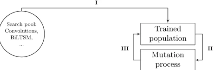
We propose XMC-NAS, a tool to automatically design architecture for the extreme multi-label classification task. Our approach relies on 3 main components: i) the embedding of the text, ii) the search of the architecture, and iii) the classifica-tion of the output. These three components form a pipeline in which components i) and iii) are fixed and are excluded from the search task. Thus, the architec-ture search task is done only on the component ii). The first component of our methods transforms the text into word-embeddings, i.e. numerical vectors, which reflect word embeddings. This step of embedding should allow the model to use these representations in order to produce more accurate prediction. The second step is the search phase for the most performing architecture, using an evolutive algorithm (c.f. Fig. 1). Finally, the last component classifies the output, into several categories. This step of classification relies on attention mechanism and fully connected layers. An overview of XMS-NAS is given in Figure 1.
Search pool: Convolutions, BiLTSM, ... Trained population Mutation process I II III
Fig. 1: I. Architectures are constructed with randomly sampled operations and then trained and evaluated, II. Sample randomly 10 architectures, and rank them by Precision@5. The most performing one is selected for mutation, III. The newly mutated architecture, is trained and evaluated. Then placed in the trained population. The oldest architecture is removed from the population.
In the following we describe in details our approach. First, we present the search space, the architecture search algorithm used and their specificities; and finally, we describe the different parts of the discovered network.
3.1 Architecture search phase
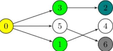
Search space. A neural network architecture, is represented in the form of a Direct Acyclic Graph (DAG). Each node of this graph represents a layer. A layer, is a single operation, which is chosen from the candidate operations set. The edges of the graph represent the data flow, each node can have only one input. The graph is constructed as follows: first the nodes are sequentially sampled (i.e. an operation is selected) to create a graph of N nodes. Then the input of a node j is selected in the set of previous nodes (i.e. nodes from 1 to j). These set is initialized with a node which represents the embedding layer. Finally, when the node j has an operation and an input, it is added to the set of the previous nodes. To have a trade-off for performance and search efficiency, we set a limit to the maximum number of previous nodes that a layer can take as input. We fix this limit at 5. Figure 2 illustrates a simple architecture, with N = 6 nodes where each node represents a layer.
Candidate operations. To build our candidate operation set we chose the most common operations in the NLP domain, which consist in a mix of Convolutional, Pooling and Recurrent Layers. We define four variants of 1D-Convolutional layer, each with different kernel size 1, 3, 5 and 7 respectively. All the convolutional layers use a stride of 1 and use padding if necessary to keep a consistent shape. The two kind of pooling layers compute the average or the maximum over the filter size, this size is set to 3 for both. Similar to the convolutional layer, the pooling layer uses a stride of 1 and uses padding if necessary. Finally, there are two popular of recurrent layers, namely the gated recurrent unit (GRU)[2] and the Long-Short Term Memory (LSTM)[3], which are able to capture long term dependencies. Specifically, we use bidirectional LSTM and GRU, so the results at time t contains information from past (backwards) and future (forward). Figure 2 illustrate how operations can be placed in the network, each color here illustrates an operation. 0 1 2 3 4 5 6
Fig. 2: Illustration of a simple architecture, with 6 layers. The node 0 represents the embedding layer. The numbers represent the sampling order of the layers. The limit of maximum number of previous layers that could be used as input is set to 5. In this example, the layer 6 could hence take as input only nodes from 1 to 5. In this scheme, different colors represent different operations.
Search Algorithm. As NAS algorithm we use the regularized evolution as described in [18]. We chose this approach because it allows us to have a fine-grained vision of the impact of each operation on the final result, this method has also demonstrated these capabilities in other areas as well. Regarding the mutation aspect, we use the same setup as described in [18], which consist mainly in two kind:
– Randomly choose an input link of an node in the network and change it by a new input.
– Randomly choose an operation in the networks and change it by a newly sampled.
Figure 2 illustrates the search algorithm, of the regularized evolution. In order to see the impact of the number of layers on the final results, a third mutation, corresponding to the addition of a new layer, has been introduced. We also aim to have a better understanding on how blocks perform together, i.e. evaluating the importance of the various operations with respect to the final results. For this purpose we have used a linear combination of weights on the output of each layer. The weights of those combination are learned during the training process. 3.2 Text embedding, Attention and classification modules
Text embedding. The embedding layer produces a fixed length representation. This layer is a word level embedding which means each words is transformed to a vector. We use the pre-trained embedding GloVe [15], which allows us to save the step of learning a new embedding from scratch. We use the 840B tokens, with a dimension 3004.
Attention module. We use a self-attention mechanism based on the one demon-strated in [7], similarly as done in [22]. The attention process helps to catch the important part of the text. This mechanism uses a vector ct which represents the relevant context for the label t, where t is in 1, . . . , T . For an input sequence of size N , the context vector is given in equation 1.
ct = N ∑ i=1 αt,ihi, (1) αt,i= eWtT·hi ∑N k=1eWt T·h k (2)
where, hi denotes the hidden representation, that is, the output of RNN encoder states or of the convolution. In the case of BiLSTM, layer hi is the concatenation of vectors from the forward−→hi and backward
←−
hi passes. The term
αt,i is called attention factor (equation (2)). The set of attention factors{αt,i} represents how much of each inputs should be considered for each output. In equation 2, Wt is the attention weight (i.e a learnable weight matrix) for the t-th label. As proposed in [12], we use here a dot product.
4
Classification module. The final part of the network is composed of 1 or 2 fully connected layers, which are used to reduce the output of the attention module. The reduced result is then fed into an output layer which classify it into different labels.
3.3 Analysis of operation importance
This section presents the linear combination weight analysis, specifically the impact of each operation on the final results, and how the operations perform together. We tackle this analysis in two steps. In the first step, we focus on the combination of operations. In the second step, we analyze the results and the impact of operations when networks become deeper.
First step: In this step, the base population is randomly initialized, i.e. the input, the operation and the skip connections, are randomly chosen. Here, we are looking which operation is the most important in the first layers by scal-ing their outputs by trainable weights. Figure 3 shows three examples of the first layers for different combinations of operations as well as the corresponding learned weights assigned to each operations. The block ”Rest of the network” represents the attention module and the chain of fully-connected. The blocks in the hatched areas of the figure 3 were not part of the mutation process and were ”constrained”. For each architecture examples, the displayed weights are the obtained means over several NAS runs. The different grey scales denote dif-ferent experiments. We observe in figure 3 that operation pairs of same kind, i.e. BiLSTM, tend to have nearly equal weights. However some trends could be noticed in the case of the two convolution combination, the convolutions with larger kernel sizes have larger weights. This effect is particularly pronounced in the case of the kernel size of 1, which reflects the necessity of sequence modeling blocks at that level. In the case of mixed operations, it turned out that BiLSTM operations systematically have larger weights. An example of a run with mixed operation is shown in the right-hand side of figure 3. More generally, we observe that architectures which contain BiLSTM at the first layer, perform better. In addition, we also found that networks with BiGRU tended to be less successful. While GRU cells are known to converge faster, LSTM cells have generally better performance.
Second step: This second stage of analysis aims to quantify the impact of the number of layers on the final results as well as the weights attributed to each operation. According to the results obtained in the first one, which show that the network with BiLSTM layers works better, in this second series, part of the population has the constraint to start with at least one BiLSTM block, which takes as input the embedding. For the impact analysis of the number of layers, we calculated the average P @5 based on the number of layers. We vary the number of layers from 2 to 6. We observe that the averaged precision is nearly constant, regardless of the number of layers in the network, with a range of results close to what we get previously. This result is corroborated by the operations weights analysis. Figure 4 shows architecture examples for different
Embedding Embedding Embedding BiLSTM Rest of the network P @5 = [0.618; 0.622] BiLSTM Conv Rest of the network P @5 = [0.56; 0.58] Conv Conv Rest of the network BiLSTM P @5 = [0.59; 0.61] 0.49 0.51 0.4 0.6 0.67 0.33
Fig. 3: Network architecture visualization with the weight applied on each oper-ation by the linear combinoper-ation during step one of search step. The weights have been averaged over multiple runs, the range of P @5 show the variation. For the middle case we also averaged over the kernel size.
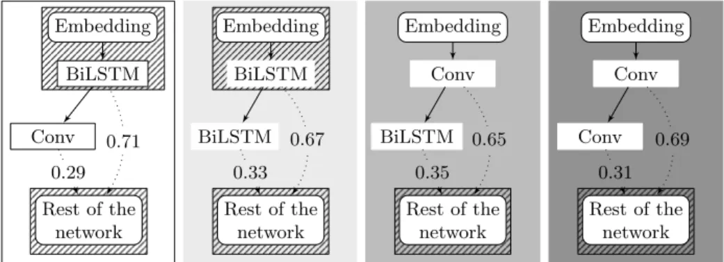
combinations of operations together with their associated weights, which are this time assigned in a sequential way. The blocks in hatched areas in figure 4 are partially or totally part of a constraint like in the previous subsection. Here, the blocks ”Rest of the network” represent the following layers in the network, not shown for the sake of clarity, and still followed by the attention module and the chain of fully connected. As previously, the displayed weights for each architecture type are the averages obtained from several NAS runs. We note in figure 4 that the weights on additional layers are small compared to those that bypass it. This trend has been observed in all experiments and suggests that, given our operations pool, additional layers does not bring much more information. BiLSTM Conv Rest of the network BiLSTM BiLSTM Rest of the network Conv BiLSTM Rest of the network Conv Conv Rest of the network Embedding Embedding Embedding Embedding
0.71 0.29 0.67 0.33 0.65 0.35 0.69 0.31
Fig. 4: Visualization of the network architecture, when the network is deeper. The dotted line represent the linear combination of all the layers outputs, with the weight applied on each outputs. The weight indicates that layers which take the embedding layer as input, have a predominant importance on the final result.
4
Experimental results
We conducted a number of experiments aimed at evaluating how the proposed XMC-NAS method can help to design an efficient neural network model for multi-label text classification.
4.1 Datasets and evaluation metrics
We conducted our study on three of the most popular XMC benchmark datasets downloaded from the XMC repository5. These datasets are considered large
scale, with the number of class labels varying from 4,000 to 30,000, which are listed from smallest to largest (in term of number of labels) by EURLex-4K, AmazonCat-13K, and Wiki10-31K summarized in Table 1. We followed the same pre=processing pipeline as used in [22]. To create the validation set we perform a split with the same random seed initialization for all experiments.
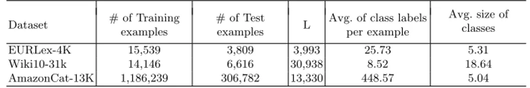
Table 1: Statistics of XMC datasets considered in our experiments. L: # of classes.
Dataset # of Training
examples
# of Test
examples L
Avg. of class labels per example Avg. size of classes EURLex-4K 15,539 3,809 3,993 25.73 5.31 Wiki10-31k 14,146 6,616 30,938 8.52 18.64 AmazonCat-13K 1,186,239 306,782 13,330 448.57 5.04
As evaluation metrics we used the Precision at k denoted by P @k, and the normalized discounted cumulative gain at k denoted by nDCG@k [4]. Both metrics are standard and widely used in the state of the art references.
4.2 Architecture search evaluation
This section presents the data and the hyper-parameters that we use the the search phase of our method. Finally, we present the most performing architecture discovered on the proxy dataset.
Parameters and data We conducted the search phase on the relatively small EURLex-4K dataset for scalability consideration, we call that a proxy dataset. In each experiment we create a base population of 20 networks. We then apply 50 rounds of mutations. Some hyper-parameters have been fixed during the training of each network, namely the learning rates were set to 0.001, and the maximum number of epochs were set to 30 epochs with early stopping. The training stops if the performance of the network does not increase during 50 consecutive steps. We use the cross-entropy loss function proposed in [22] and [10] for training the models.
5
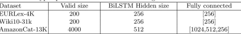
The discovered architecture The architecture found by XMC-NAS, is made of two BiLSTM which take the same inputs and holds their own weights and features. The output of the two BiLSTM is then concatenated along the hidden dimension, and given as input of the self-attention block. Finally we use a chain of fully connected network to classify the sequence. For the training detail we use the same as presented in the previous paragraph and more dataset related training details are presented in table 2.
Table 2: Hyper-parameters used for the training of the discovered model.
Dataset Valid size BiLSTM Hidden size Fully connected
EURLex-4K 200 256 [256]
Wiki10-31k 200 256 [256]
AmazonCat-13K 4000 512 [1024,512,256]
The architecture of the network found by XMC-NAS is presented in Figure 5.
Embedding
BiLSTM
BiLSTM
Concat Attention module Classification module
Fig. 5: The discovered network by XMC-NAS, is composed of two BiLSTM which results are concatenated, then passed in an attention module and finally in a part of fully connected layers.
4.3 Performance evaluation
In this section we will present the results obtained by the XMC-NAS discovered architecture (Figure 5) on various XMC datasets (Table 1). First we present the results obtained on the EURLex-4K dataset used for the search phase, also named proxy dataset. Finally we evaluate the performance of this discovered architecture, transferred on the other datasets. To train our network we use 2 Nvidia GV100, with data parallelism training. We compare the results of our method to the most representative methods on XMC (with the implementation and the results provided by the authors). Some of theses techniques are deep learning base like MLC2Seq[14], XML-CNN[10], Attention-XML[22]. The oth-ers are more specific techniques, AnnexML[19], DiSMEC[1], PfastreXML[4],and Parabel[17].
EURLex-4K results On this dataset, the network got an improvement re-garding the precision at k to the state of the art. As presented in the left side
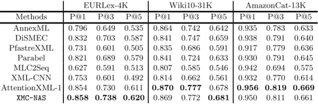
Table 3: Comparison performance table on three datasets. Our methods surpass the state of the art in 4 cases, and get competitive results that really close to the state of the art otherwise.
EURLex-4K Wiki10-31K AmazonCat-13K Methods P@1 P@3 P@5 P@1 P@3 P@5 P@1 P@3 P@5 AnnexML 0.796 0.649 0.535 0.864 0.742 0.642 0.935 0.783 0.633 DiSMEC 0.832 0.703 0.587 0.841 0.747 0.659 0.938 0.791 0.640 PfastreXML 0.731 0.601 0.505 0.835 0.686 0.591 0.917 0.779 0.636 Parabel 0.821 0.689 0.579 0.841 0.724 0.633 0.930 0.791 0.645 MLC2Seq 0.627 0.591 0.513 0.807 0.585 0.546 0.942 0.694 0.575 XML-CNN 0.753 0.601 0.492 0.814 0.662 0.561 0.932 0.770 0.614 AttentionXML-1 0.854 0.730 0.611 0.870 0.777 0.678 0.956 0.819 0.669 XMC-NAS 0.858 0.738 0.620 0.869 0.772 0.681 0.950 0.811 0.661
of the Table 3 we got an improvement on P@1, P@3 and P@5. A significant improvement is obtained on precision at 3 and 5, where we get 0.738 and 0.620 respectively compared to 0.730 and 0.611 before. The figure 6a presents the evo-lution of P@5 and the nDCG@5 on the validation set with respect to the number of epochs. We observe on figure 6a that our network have a faster convergence. The results is obtained around 15 epochs and after this point, we only get small improvement which indicates that the network might overfit.
Architecture transfer results We train and evaluate the discovered architec-ture following the same training procedure as defined in Section 4.2 and using the hyper-parameters presented in Table 2 on the two other datasets. The mid-dle and right side of table 3 show the comparison of the architecture found by
0 5 10 15 20 25 30 Epochs 0.0 0.1 0.2 0.3 0.4 0.5 0.6 0.7 Metrics XMC-NAS nDCG@5 XMC-NAS P@5 AttentionXML-1 nDCG@5 AttentionXML-1 P@5 (a) EURLex-4K 0 5 10 15 20 25 30 Epochs 0.0 0.1 0.2 0.3 0.4 0.5 0.6 0.7 Metrics XMC-NAS nDCG@5 XMC-NAS P@5 AttentionXML-1 nDCG@5 AttentionXML-1 P@5 (b) Wiki10-31K
Fig. 6: Plot of the nDCG@5 and P@5 on the validation set, on two different datasets. We notice, the discovered architecture have a faster convergence com-pared to the current state of the art. In the 6a our methods get better final results, in 6b the final results are close, the final results are obtained around 15 epochs.
XMC-NAS on EURLex-4K with others methods. We notice that the discovered architecture transferred to larger datasets get close results to the current state of the art, even slightly surpassing them like on Wiki10-31K for P @5. Moreover we notice in Fig. 6b that our methods still have a faster convergence, the same trend as on the proxy dataset on which we searched the architecture.
5
Summary & Outlook
We have presented in this work an automated method to discover architecture for the specific task of extreme multi-label classification, based on the regularized evolution [18] and with a domain-oriented pool of operations. This method has found architectures that provided competitive results with the existing state of the art methods [22], and in some cases overpassed them. Moreover, our method showed faster convergence rates on all datasets. Moreover, trainable weights have been introduced on each operations of the pool in order to provide more understanding on the impact of each architecture blocks. Many directions are possible as future steps. This involves creating a method that can manage large datasets while still speeding up the search process. The use of transfer learning to speed up the training portion may be a partial solution to the latter point.
Acknowledgment
This work has been partially supported by MIAI@Grenoble Alpes (ANR-19-P3IA-0003).
References
1. Babbar, R., Sch¨olkopf, B.: Dismec: Distributed sparse machines for extreme multi-label classification. In: Proceedings of the Tenth ACM International Conference on Web Search and Data Mining. pp. 721–729 (2017)
2. Cho, K., Van Merri¨enboer, B., Gulcehre, C., Bahdanau, D., Bougares, F., Schwenk, H., Bengio, Y.: Learning phrase representations using rnn encoder-decoder for statistical machine translation. arXiv preprint arXiv:1406.1078 (2014)
3. Hochreiter, S., Schmidhuber, J.: Long short-term memory. Neural computation
9(8), 1735–1780 (1997)
4. Jain, H., Prabhu, Y., Varma, M.: Extreme multi-label loss functions for recom-mendation, tagging, ranking & other missing label applications. In: Proceedings of the 22nd ACM SIGKDD International Conference on Knowledge Discovery and Data Mining. pp. 935–944 (2016)
5. Jin, H., Song, Q., Hu, X.: Auto-keras: An efficient neural architecture search system. In: Proceedings of the 25th ACM SIGKDD International Conference on Knowledge Discovery & Data Mining. pp. 1946–1956 (2019)
6. Kitano, H.: Designing neural networks using genetic algorithms with graph gener-ation system. Complex Systems 4 (1990)
7. Lin, Z., Feng, M., Santos, C.N.d., Yu, M., Xiang, B., Zhou, B., Bengio, Y.: A struc-tured self-attentive sentence embedding. arXiv preprint arXiv:1703.03130 (2017)
8. Liu, C., Zoph, B., Neumann, M., Shlens, J., Hua, W., Li, L.J., Fei-Fei, L., Yuille, A., Huang, J., Murphy, K.: Progressive neural architecture search. In: Proceedings of the European Conference on Computer Vision (ECCV). pp. 19–34 (2018) 9. Liu, H., Simonyan, K., Yang, Y.: Darts: Differentiable architecture search. arXiv
preprint arXiv:1806.09055 (2018)
10. Liu, J., Chang, W.C., Wu, Y., Yang, Y.: Deep learning for extreme multi-label text classification. In: Proceedings of the 40th International ACM SIGIR Conference on Research and Development in Information Retrieval. pp. 115–124 (2017) 11. Liu, X., Gao, J., He, X., Deng, L., Duh, K., Wang, Y.Y.: Representation learning
using multi-task deep neural networks for semantic classification and information retrieval (2015)
12. Luong, M.T., Pham, H., Manning, C.D.: Effective approaches to attention-based neural machine translation. arXiv preprint arXiv:1508.04025 (2015)
13. Maziarz, K., Tan, M., Khorlin, A., Chang, K.Y.S., Jastrzebski, S., de Laroussilhe, Q., Gesmundo, A.: Evolutionary-neural hybrid agents for architecture search. arXiv preprint arXiv:1811.09828 (2018)
14. Nam, J., Menc´ıa, E.L., Kim, H.J., F¨urnkranz, J.: Maximizing subset accuracy with recurrent neural networks in multi-label classification. In: Advances in neural information processing systems. pp. 5413–5423 (2017)
15. Pennington, J., Socher, R., Manning, C.D.: Glove: Global vectors for word repre-sentation. In: Proceedings of the 2014 conference on empirical methods in natural language processing (EMNLP). pp. 1532–1543 (2014)
16. Pham, H., Guan, M.Y., Zoph, B., Le, Q.V., Dean, J.: Efficient neural architecture search via parameter sharing. arXiv preprint arXiv:1802.03268 (2018)
17. Prabhu, Y., Kag, A., Harsola, S., Agrawal, R., Varma, M.: Parabel: Partitioned label trees for extreme classification with application to dynamic search advertising. In: Proceedings of the 2018 World Wide Web Conference. pp. 993–1002 (2018) 18. Real, E., Aggarwal, A., Huang, Y., Le, Q.V.: Regularized evolution for image
clas-sifier architecture search. In: Proceedings of the aaai conference on artificial intel-ligence. vol. 33, pp. 4780–4789 (2019)
19. Tagami, Y.: Annexml: Approximate nearest neighbor search for extreme multi-label classification. In: Proceedings of the 23rd ACM SIGKDD international con-ference on knowledge discovery and data mining. pp. 455–464 (2017)
20. Tan, C., Sun, F., Kong, T., Zhang, W., Yang, C., Liu, C.: A survey on deep transfer learning. In: International conference on artificial neural networks. pp. 270–279. Springer (2018)
21. Yang, P., Sun, X., Li, W., Ma, S., Wu, W., Wang, H.: Sgm: sequence generation model for multi-label classification. arXiv preprint arXiv:1806.04822 (2018) 22. You, R., Dai, S., Zhang, Z., Mamitsuka, H., Zhu, S.: Attentionxml: Extreme
multi-label text classification with multi-multi-label attention based recurrent neural networks. arXiv preprint arXiv:1811.01727 (2018)
23. Zhang, X., Zhao, J., LeCun, Y.: Character-level convolutional networks for text classification. In: Advances in neural information processing systems. pp. 649–657 (2015)
24. Zhou, C., Sun, C., Liu, Z., Lau, F.: A c-lstm neural network for text classification. arXiv preprint arXiv:1511.08630 (2015)
25. Zoph, B., Le, Q.V.: Neural architecture search with reinforcement learning. arXiv preprint arXiv:1611.01578 (2016)
26. Zoph, B., Vasudevan, V., Shlens, J., Le, Q.V.: Learning transferable architectures for scalable image recognition. In: Proceedings of the IEEE conference on computer vision and pattern recognition. pp. 8697–8710 (2018)