Design and tracking of desirable trajectories in the image space by integrating mechanical and visibility constraints

HAL Id: inria-00352136

https://hal.inria.fr/inria-00352136

Submitted on 12 Jan 2009

HAL is a multi-disciplinary open access

archive for the deposit and dissemination of

sci-entific research documents, whether they are

pub-lished or not. The documents may come from

teaching and research institutions in France or

abroad, or from public or private research centers.

L’archive ouverte pluridisciplinaire HAL, est

destinée au dépôt et à la diffusion de documents

scientifiques de niveau recherche, publiés ou non,

émanant des établissements d’enseignement et de

recherche français ou étrangers, des laboratoires

publics ou privés.

Design and tracking of desirable trajectories in the

image space by integrating mechanical and visibility

constraints

Youcef Mezouar, François Chaumette

To cite this version:

Youcef Mezouar, François Chaumette. Design and tracking of desirable trajectories in the image space

by integrating mechanical and visibility constraints. IEEE Int. Conf. on Robotics and Automation,

ICRA’01, 2001, Seoul, South Korea. pp.731-736. �inria-00352136�

Proceedings of the 2001 IEEE

International Conference on Robotics 8 Automation Seoul, Korea. May 21-26, 2001

Design and Tracking of Desirable Trajectories in the Image Space

by Integrating Mechanical and Visibility Constraints

Youcef Mezouar

Franqois Chaumette

Youcef.Mezouar@irisa.fr

Francois.Chaumette@irisa.fr

IRISA - INRIA Rennes

Campus de Beaulieu,

35042

Rennes Cedex, France

Abstract

Since image-based visual servoing is a local feedback control solution, it requires the definition of intermediate subgoals in the sensor space at the task planning level. In this paper, we describe a general technique f o r specifying and tracking trajectories of an unknown object in the cam- era image space. First, physically valid C2 image trajec- tories which correspond to quasi-optimal 3 0 camera tra- jectory (approaching as much as possible a straight line) are peqormed. Both mechanical ('joint limits) and visibil- ity constraints are taken into account at the task planning

level. The good behavior of Image-based control when de- sired and current camera positions are closed is then ex- ploited to design an efJicient control scheme. Real time experimental results using a camera mounted on the end effector of a six d - o f robot confirm the validity of our ap- proach.

1 Introduction

Classical approaches, using visual information in feed- back control loops [6, 81, are point to point-based, i.e the robot must reach a desired goal configuration starting from a given initial configuration. In such approaches, a globally stabilizing feedback control solution is required. However if the initial error is large, such a control may product er- ratic behavior especially in presence of modeling errors. For a very simple case, Cowan and Koditschek describe in [3] a globally stabilizing method using navigation function. By composing the error function of 3D Cartesian features and image features, Malis et a1 propose a globally stabi- lizing solution called 2 1/2 D visual servoing for general

setup [l 11. Classical image-based visual servoing is a lo- cal control solution. It thus requires the definition of inter- mediate subgoals in the sensor space at the task planning level if the initial error is large. In this approach the robot effector is controlled so that the image features converge

tory in the 3D Cartesian space is not controlled. Such a control can thus provide inadequate robot motion leading to no optimal or no physically valid robot trajectory [l]. However, it is well known that image-based control is lo- cally stable and robust with respect to modeling errors and noise perturbations. The key idea of our work is to use the local stability and robustness of image-based servoing by specifying trajectories to follow in the image. Indeed, for a trajectory following a local control solution works prop- erly since current and desired configurations remain close. Only few papers deal with path planning in image space. In [7] a trajectory generator using a stereo system is pro- posed and applied to obstacle avoidance. An alignment task using intermediate views of the object synthesized by image morphing is presented in [16]. A path planning for a straight-line robot translation observed by a weakly cali- brated stereo system is performed in [ 141. In previous work

[ 121, we have proposed a potential field-based path plan- ning generator that determines the trajectories in the image of a set of points lying on a planar target. In this paper,

we propose to plan the trajectory of an unknown and not

necessarily planar object. Both mechanical (joint lim- its) and visibility constraints are taken into account. Con-

trarily to others approaches [2, 131 exploiting the robot re- dundancy, the mechanical and visibility constraints can be ensured even if all the robot degrees of freedom are used to realize the task.

More precisely, we plan the trajectory of s = [pT

. . .

p;lT,

composed of the 2 x n image coordinates of n points

M j lying on an unknown target, between the initial con-

figuration si = [pz

. .

.

p;JT and the desired one s* = [pTT

. . .

pLT]'. Our approach consists of three phases. In the first one, the discrete geometric camera path (that ensures the physical validity of the image trajectories) is

performed as a sequence of N intermediate camera poses

which approaches as much as possible a straight line in the Cartesian space. In this phase, the mechanical and visi-

bility constraints are introduced. In the second one, the discrete geometric trajectory of the target in the image and the discrete geometric trajectory of the robot in the joint space are obtained from the camera path. Finally, contin- uous and derivable geometric paths in the image with an associated timing law s*

( t )

is generated and tracked using an image-based control scheme.

The paper is organized as follows. In Section 2, we re- call some fundamentals. The mcthod of path planning is presented in Section 3. In Section 4, we show how to use an image-based control approach to track the trajectories. In section 5, a timing law is associated with the geometric path. The experimental results are given in Section 6.

2 Potential field method

Our path planning strategy is based on the potential field method [9, lo]. In this approach the robot motions are un- der the influence of an artificial potential field ( V ) defined as the sum of an attractive potenlial (V,) pulling the robot toward the goal configuration (Y,) and a repulsive poten- tial

(V,)

pushing the robot away from the obstacles. Mo- tion planning is performed in an iterative fashion. At each iteration an artificial force F ( Y ) , where the 6 x 1 vector Y represents a parameterization of robot workspace, is in- duced by the+potential fyction. This force is defined as F ( Y ) = -VV where

VV

denotes the gradient vector of V at Y. Each segment of the path is oriented along the negated gradient of the potential Function:

I

where

k

is the increment index and E k a positive scaling factor denoting the length of the k t h increment. In our case, the control objective is formulated to transfer the system to a desired point in the sensor space and to provide robot motion satisfying the following c'mstraints:

1. all the considered image features remain in the camera field of view

2. the robot joint positions remain between their limits To deal with the first constraint, a repulsive potential V r s ( s ) is defined in the image. The second constraint is introduced through a repulsive potential V,, (9) defined in the joint space. The total force is given by:

F =

- 9 v a k

- y k f K s k - XkeVrqk

The scaling factors 'yk and X k allow us to adjust the relative influence of the different forces.

3

Trajectories planning

We consider that the target model is not available. In this case the camera pose can not be estimated. Only a

scaled Euclidean reconstruction can be obtained by per- forming a partial pose estimation as described in the next subsection. This partial pose estimation and the relations linking two views of a static object are then exploited to design a path of the projection of the unknown object in the image.

3.1

Scaled Euclidean reconstruction

Let

3*

and

F

be the frames attached to the camera in its desired and current positions. The rotation matrix and the translation vector between

3

and

F*

are denoted

*R,

and *t,, respectively. A target point

M j with ho-

mogeneous coordinates Mj = [ X j Yj Zj 11 (resp. M;) in

F

(resp. 3*) is projected in the camera image onto a point with homogeneous normalized and pixel coordinates

mj = [ z j y j l I T (resp. m;) and pj =

[q

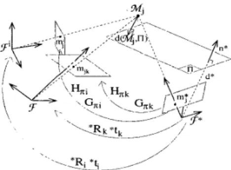
w j 1IT = Amj (resp. p;), where A denotes the intrinsic parameters ma- trix of the camera.

Consider a 3D reference plane

II

given in

F*

by

6

= [n* -

@I,

where n* is its unitary normal in

F*

and d* is the distance from

II

to the origin of

3*

(see Fig. 1). It is well known that there is a projective homography matrix G, such that:

a j p j = G,p5

+

pje with e = -A

*RT

*t, (2) where aj is a positive scaling factor and pj is a scaling fac- tor null if the target point is linked with

II.

More precisely, if we define the signed distance d ( M j ,

II)

= 7r M;, we

have:

If at least four matched points belonging to

II

are known, G , can be estimated by solving a linear system. Else, at least height points

(3

points to define

II

and

5

outside of

II)

are necessary to estimate the homography matrix by using for example the linearized algorithm proposed in [ 1 11. As- suming that the camera calibration is known, the Euclidean homography H, of plane

II

is estimated as follow:

H, = A-lG,A (4)

and it can be decomposed into a rotation matrix and a rank 1 matrix [5]:

( 5 )

* t c

H,

=

*RF

-

*RTtd*n*T

where

td+

= - d*

From H, and the image features, it is thus possible to de- termine the camera motion parameters (that is the rotation

*R,

and the scaled translation t p ) and the vector n* [5]. The structure of the observed scene can also be determined. For example, the ratio between the Z-coordinates of a 3D point M j expressed in 3 and the distance d * , pj = Zj/d*

can be obtained from

*R,,

tp and the image features [ 1 l].These parameters are important since they are used in the path planning generator and in the control scheme.

Mi

Figure 1: Scaled camera trajectory

3.2

Scaled

3-D

Cartesian trajectory

The homography G,i is computed from si and s * . Ac- cording to (4), we obtain H,i. Then n* is estimated, as well as the rotation *Ri and the scaled translation td’i = *ti/d* between

F i

(frame linked to the camera in its ini- tial position) and

F*.

If we choose as partial parameteri-

zation of the workspace Y = [tz* where U and B

are the normalized rotation axis and the rotation angle ex- tracted from *R,, we obtain at the initial and desired robot configurations Yi = [tz*i (u6)TIT and Y, = O c X 1 .

We thus have to determine a path starting at the initial con- figuration Y k = ~ = Y i and ending at Y * = OS 1 .

3.3

Trajectories in the joint space

To anticipate the possible encounter of a joint limit and to avoid it, we have to estimate the trajectory of the robot in the joint space. Indeed, the value of the joint coordinates at each iteration is used in the computation of the repul- sive potential related to the joint limits avoidance. If the manipulator position in the joint space is represented by

q = [ql

. . .

q,]*, we have:

where J(q) and M y ( @ ) denote the robot Jacobian and the parameterization Jacobian respectively. The parame- terization Jacobian can be computed directly from Y and d* [12]:

1

d**RT

03x3 My(d*) =

[

03x3

The computation of L i l can be found in [ 111’:

The trajectory of the robot coordinates in the joint space are then obtained from the trajectory of Y by a linearization of

‘ l u ] ~ denotes the antisymmetric matrix associated to the vector U

(6) around q k

qk+l = q k

+

J+(qk)MY,(d*)(Tk+l -

yk)

3.4

Image trajectories

The homography matrix G T k of plane

Il

relating the

current and desired images can be computed from Y k us- ing (4) and (5):

G , k = A( *RT - *Rztd*kn*T)A-l (7) According to (2) the image coordinates of the points M j at time IC are given by:

where (refer to (2) and ( 3 ) ) :

using the previous relation, (8) can be rewritten:

Furthermore, if the relation (9) is applied between the de- sired and initial camera positions, we obtain *:

h P 3 ~ IIGripj” A pjill (A *RTt,j*i), JIA*RTt,j*i A pjiJI

(10) The equations (7), (9) and (10) allow to compute p j k p j k

from Y k and the initial and desired visual features. The image coordinates pjk are then computed by dividing

p j p j k by its last component. Furthermore, the ratio pjk, which will be used in the repulsive force and in the control law, can easily be obtained from Y k and m j k = A-lpjk.

3.5

Reaching the goal

1

M y s i g n ( ‘

z;

”

-The potential field V, is defined as a parabolic function in order to minimize the distance between the current po- sition and the desired one:

V,(Y)

=

fllY

- Y,1I2 =

IlY

112.

The function V, is positive or null and attains its minimum at Y * where V, (Y

*)

=

0.

It generates a force Fa that converges linearly toward the goal configuration:

F,(Y) = -vV, = - Y (11) When the repulsive potentials are not needed, the transition equation can be written (refer to (1) and (1 1)):

Yk+l = (1 -

&)

Tk

Thus, y k is lying on the straight line passing by and

Y*. As a consequence, the translation performed by the camera is a real straight line sincl: Yk is defined with re- spect to a motionless frame (that is

F*).

However, the ob- ject can get out of the camera field of view and the robot can attain its joint limits along thilj trajectory. In order that the object remains in the camera field of view and that the robot remains in its mechanical limits, two repulsive forces are introduced by deviating the camera trajectory when needed.

3.6

Mechanic and visibility constraints

A. Joint limits avoidance. The robot configuration q is

called acceptable if each of its components is sufficiently far away from its corresponding joints limits. We note

C

the subset of the joint space of acceptable configurations. The repulsive potential

V,,

(9) is defined as:

m

qjmin and qj,,, being the minimum and the maximum allowable joint values for the j t h joint. The artificial repul- sive force deriving from V,, is :

The previous equation can be rewritten:

B. Visibility constraint. One way to create a potential

barrier around the camera field of view is to define VrS as an increasing function of the distance between the object projection and the image limits. A general description of such a function is given in [ 121.

4

Performing

C2 timing 1:aw

In the previous subsection we have obtained discrete trajectories. In order to design continuous and derivable curves and thus to improve the dynamic behavior of the system, we use cubic B-spline interpolation. The spline in- terpolation problem is usually stated as: given data points

S

= { s k / k E 1 . . . N } and a set of parameter values

7

= { t k / k E 1

.-.N},

we have to determine a cubic B- spline curve

s ( t )

such that

S ( t k )

=

S k , v t k .

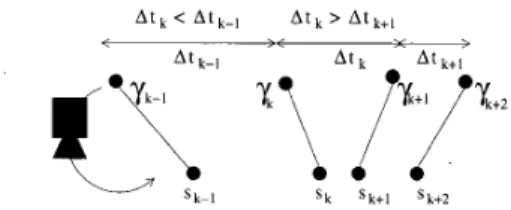
In practice, parameter values are rarely given. In our case, we can ad- just them to the distribution of the vector of image features

S k or using the distribution of the Icamera positions Y k . In order to control efficiently the camera velocity, it is more

reasonable to use the distribution of the camera positions. The time values are thus chosen spacing proportionally to the distances between camera positions (see Fig. 2):

Atk - t k + l - t k - I l y k + l - Y k l l Atk+l t k + 2 - t k + l I I y k + 2 - y k + l I )

- -

Considering the transition equation (l), we obtain:

T being the time between two consecutive frames (cho- sen for example as the video rate). In practice, &k is cho-

sen constant, we thus have t k = kT. Given the data vectors s k and the parameters values t k , the image data can be interpolated by using a natural cubic B-spline in- terpolation and we obtain a C2 function

s ( t )

defined for

(IC

-

1 ) A T 5 t 5 kAT

by:

S ( t )

= A k t 3

+

Bkt2 f Ckt f Dk (12) where the n x n diagonal matrices As, Bk, c k , Dk are obtained from S and

7 .

Finally, the ratio p appears in the control law. By using the same process,

r ( t )

=

[ p 1 ( t )

.

+

p n ( t ) ]

is computed from

R = { r k / k E

l . . . N } a n d

7 .

A t k < A t k - , A t k > A t k + ,

< v _>

A t k A t k t l

sk sk+l sk+Z

Figure 2: Controlling the time along the camera trajectory

5 Tracking the trajectories

To track the trajectories using an image-based control scheme, we use the task function approach introduced by Samson et a1 in [15]. A vision-based task function e to be regulated to 0 is defined by [4]:

e =

Z + ( s ( r ( t ) )

-

s * ( t ) )

The time varying vector

s * ( t )

is the desired trajectory of s computed in the previous sections. L denotes the well known interaction matrix (also called image Jacobian) and the matrix

E+

represents the pseudo-inverse of a chosen model of L. More precisely, when s is composed of the image coordinates of n points, two successive rows of the image Jacobian are given by:

The value of L at the current desired position is used for

2,

that is

5

= L(s*(t),I'*(t),d^*),

d^*

being an estimated value of d* and I?* ( t ) = [&)

. . .

p k ( t ) ] is the obtained trajectory for I?. An exponential decay of e toward 0 can be obtained by imposing e = -Xe (X being a proportional gain), the corresponding control law is:

de

T, = -Xe - -

dt

where T, is the camera velocity sent to the robot controller. If the target is known to be motionless, we have =

-"%

and the camera velocity can be rewritten:

..

as*

T, = -Xe

+

Lf-

d t

where thc term

c+g

allows to compensate the tracking

error. More precisely, we have from (1 2):

= 3Akt2

+

2Bkt

+

Ck for ( k - 1 ) A T

5

t

5

k A T

This control law posses nice degrees of robustness with respect to modeling errors and noise perturbations since the error function used as input remains small and is directly computed from visual features.

6

Experimental Results

The proposed method has been tested on a six d-o-f eye-in-hand system. The specified visual task consists in

a positioning task with respect to an unknown object. The target is a marked object with nine white marks lying on

three differerent planes (see Fig. 3). The extracted visual features are the image coordinates of the center of gravity of each mark. The images corresponding to the desired and initial camera positions are given in Figs. 3(a) and 3(b) re- spectively. The corresponding camera displacement is very important

( t , =

820mm,

t ,

= 800mm,

t ,

= 450mm,

(uB), = 37dg,

(ue),

= 45dg, (U@), = 125dg). In this

case classical image-based and position-based visual ser- voing fail.

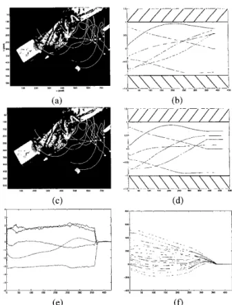
On all the following plots, joint positions are normalized between [-1;1], where -1 and 1 represents the joint limits. In order to emphasize the importance of the introduced constraints in the trajectories, we first perform the path planning without repulsive potential. The results are given in Fig. 3. We can see that the visual features get out largely of the camera field of view (Fig.3(c)) and the axis 45 attains its joint limit (Fig.3(d))

.

Then, only the repulsive poten- tial associated to the visibility constraint has been activated (see Fig. 4). In that case, even if the visibility constraint is ensured (Fig 4(a)) the servoing can not be realized be- cause the axis 45 reaches its joint limit (Fig 4(b)). In Fig. 5, the two repulsive potentials are activated. The target re- mains in the camera field of view (see Fig. 5(a) and 5(c))

and all axes avoid their joint limit (see Fig. 5(b) and 5(d)). We can notice that the planned trajectories and the realized trajectories in the image are almost similar, that shows the efficiency of our control scheme. The error on the image coordinates of each target point between its current and de- sired location is given in Fig. 5(f). We can note the con- vergence of the coordinates to their desired value, which demonstrates the correct realization of the positioning task.

Figure 3: (a) Initial and (b) Desired images; Planned tra- jectories without any repulsive potential (c) in the image,

(d) in the joint space

Figure 4: Planned trajectories without repulsive potential associated to the joint limits avoidance (a) in the image,

(b) in the joint space

7

Conclusion

In this paper, we have presented a method ensuring the convergence for all initial camera position. By coupling an image-based trajectory generator and an image-based servoing, the proposed method extends the well known stability of image-based servoing when initial and desired camera location are close to the case where they are dis- tant. The obtained trajectories provide some good expected

properties. First, along these trajectories the target remains in the camera field of view and the robot remains in its mechanical limits. Second the corresponding robot mo- tion is physically realizable and the camera trajectory is a

straight line outside the area where the repulsive forces are needed. Experimental results show the validity of our ap- proach. Future work will be devoted to generate the trajec- tories in image space of complex features in order to apply our method to complex objects.

References

[l] E Chaumette. Potential problems of stability and con- vergence in image-based and pclsition-based visual servo- ing. The ConJluence of Vision cmd Control D. Kriegman,

G. Hager; A. Morse (eds), LNClS Series, Springer Verlag,

237:66-78, 1998.

[2] E Chaumette and E. Marchand. A new redundancy-based iterative scheme for avoiding joint limits: Application to visual sevoing. In Proc. IEEE lnt. Con$ on Robotics and

Automation, volume 2, pages 1’720-1725, San Francisco, California, April 2000.

[3] N.J. Cowan and D.E. Koditschelc. Planar image based vi-

sual servoing as a navigation prc’blem. IEEE International

Conference on Robotics and Automation, pages 61 1-617, May 1999.

[4] B. Espiau, E Chaumette, and P. Rives. A new approach to visual servoing in robotics. IEEE Trans. on Robotics and

Automation, 8(3) : 313-326, 1992.

[5] 0. Faugeras and E Lustman. Motion and structure from mo- tion in a piecewise planar environment. Int. Journal of Pat-

tern Recognition and Artificial htelligence, 2(3):485-508, 1988.

[6] K. Hashimoto. Visual Sewoing: Real Time Control of Robot

Manipulators Based on Visual Sensory Feedback. World Scientific Series in Robotics ancl Automated Systems, Vol 7,World Scientific Press, Singapor, 1993.

[7] K. Hosoda, K. Sakamoto, and hl. Asada. Trajectory gen- eration for obstacle avoidance of uncalibrated stereo visual servoing without 3d reconstruction. Proc. IEEE/RSJ Int.

Conference on Intelligent Robots and Systems, 1 (3):29-34, August 1995.

[SI S . Hutchinson, G.D. Hager, and P.I. Corke. A tutorial on visual servo control. IEEE Trans. on Robotics and Automa-

tion, 12(5):651-670, octobre 19SI6.

[9] 0. Khatib. Real time obstacle avoidance for manipula- tors and mobile robots. Int. Journal of Robotics Research,

5(1):90-98, 1986.

[lo] J. C. Latombe. Robot Motion Planning. Kluwer Academic Publishers, 1991.

[ 111 E. Malis and E Chaumette. 2 lL! d visual servoing with re- spect to unknown objects through a new estimation scheme of camera displacement. Internaiional Journal of Computer Vision, June 2000.

Figure 5: Planned trajectories with both repulsive potential (a) in the image, (b) in the joint space; realized trajectories (c) in the image, (d) in the joint space, (e) camera trans- lational ( c d s ) and rotational (dg/s) velocities versus itera- tion number,

(0

errors in

the image

versus

iteration number

[12] Y. Mezouar and E Chaumette. Path planning in image space for robust visual servoing. IEEE Int. Conference on

Robotics and Automation, 3:2759-2764, April 2000.

[13] B.J. Nelson and P.K. Khosla. Strategies for increasing the tracking region of an eye-in-hand system by singularity and joint limits avoidance. Int. Journal of Robotics Research,

14(3):255-269, June 1995.

[14] A. Ruf and R. Horaud. Visual trajectories from uncalibrated stereo. IEEE International Conference on Intelligent Robots

and Systems, pages 83-91, 1997.

[15] C. Samson, B. Espiau, and M. Le Borgne: Robot Control

: The Task Function Approach. Oxford University Press, 1991.

[ 161 R. Singh, R. M. Voyle, D. Littau, and N. P. Papanikolopou- 10s. Alignement of an eye-in-hand system to real objects using virtual images. Workshop on Robust Vision for Vision- Based Control of Motion, IEEE Int. Conj on Robotics and Automation, May 1998.