THE SEASONAL EFFECT ON THE CHINESE GOLD MARKET USING AN EMPIRICAL ANALYSIS OF THE SHANGHAI GOLD EXCHANGE

(1)

HAL Id: hal-02905216

https://hal.archives-ouvertes.fr/hal-02905216

Submitted on 5 Feb 2021

HAL is a multi-disciplinary open access

archive for the deposit and dissemination of

sci-entific research documents, whether they are

pub-lished or not. The documents may come from

teaching and research institutions in France or

abroad, or from public or private research centers.

L’archive ouverte pluridisciplinaire HAL, est

destinée au dépôt et à la diffusion de documents

scientifiques de niveau recherche, publiés ou non,

émanant des établissements d’enseignement et de

recherche français ou étrangers, des laboratoires

publics ou privés.

THE SEASONAL EFFECT ON THE CHINESE GOLD

MARKET USING AN EMPIRICAL ANALYSIS OF

THE SHANGHAI GOLD EXCHANGE

Bing Xiao, Philippe Maillebuau

To cite this version:

Bing Xiao, Philippe Maillebuau. THE SEASONAL EFFECT ON THE CHINESE GOLD

MAR-KET USING AN EMPIRICAL ANALYSIS OF THE SHANGHAI GOLD EXCHANGE. EURASIAN

JOURNAL OF ECONOMICS AND FINANCE, 2020, 8 (2), pp.104-114. �hal-02905216�

(2)

See discussions, stats, and author profiles for this publication at: https://www.researchgate.net/publication/343117473

THE SEASONAL EFFECT ON THE CHINESE GOLD MARKET USING AN

EMPIRICAL ANALYSIS OF THE SHANGHAI GOLD EXCHANGE

Article in Eurasian Journal of Economics and Finance · July 2020

DOI: 10.15604/ejef.2020.08.02.005 CITATIONS 0 READS 49 2 authors, including: Bing Xiao

Université Clermont Auvergne

15PUBLICATIONS 21CITATIONS

SEE PROFILE

All content following this page was uploaded by Bing Xiao on 23 July 2020.

(3)

Eurasian Journal of Economics and Finance, 8(2), 2020, 104-114

DOI: 10.15604/ejef.2020.08.02.005

EURASIAN JOURNAL OF ECONOMICS AND FINANCE

www.eurasianpublications.com

THE SEASONAL EFFECT ON THE CHINESE GOLD MARKET USING AN

EMPIRICAL ANALYSIS OF THE SHANGHAI GOLD EXCHANGE

Bing Xiao

Corresponding Author: University of Clermont Auvergne, France Email: bing.xiao@uca.fr

Philippe Maillebuau

University of Clermont Auvergne, France Email: philippe.maillebuau@uca.fr

Received: May 19, 2020 Accepted: June 26, 2020

Abstract

Gold is considered as a hedge against inflation, it offers an opportunity for portfolio diversification. This paper examines the recent evolution of seasonal anomalies in the Chinese Gold market. It studies the day of the week effect and the monthly effect through gold prices at the Shanghai Gold Exchange (SGE) over the 2002 to 2016 period. We investigate seasonal patterns in economically favorable times and unfavorable times by using a UCM model and an ARCH model. The reforms in regulations have rendered the Chinese financial market more efficient, in such cases; we expect an alteration in seasonal anomalies in the Chinese Gold market. However, it would seem that seasonality does exist in the Chinese Gold Market. The Monday returns have been positive and the Tuesday returns have been negative for the whole period. We also highlight that January and February generate the best returns. The return in the middle of the year is negative. This paper contributes to the existing finance literature by investigating the anomalies during the recent period. Although in the Chinese stock market, the seasonal anomalies persist, the index may be efficient despite the regularity in price formation, in this case, a study over a more recent period is necessary.

Keywords: Gold, ARCH, GARCH, Shanghai Gold Exchange, Seasonality, Chinese Calendar,

Return, Volatility

JEL Classification: C53, C58, G17, G12, G14

1. Introduction

In developed stock markets, anomalies are a well-documented stylized fact. The cross-sectional stock returns are among the most robust findings. There are two sorts of anomalies: the cross-sectional stock anomalies, for example the size effect, Book to Market anomaly, etc. and the seasonal effect, for example the January effect, the week effect, etc. The issue of anomalies generates a large amount of interest in academic circles. The major reason is theoretical: if it were possible to show that investment strategy based on anomalies is capable of systematically

(4)

Xiao & Maillebuau / Eurasian Journal of Economics and Finance, 8(2), 2020, 104-114

105

beating the market, the efficient market theory would be faulty. The regulations and the attitudes of regulators have rendered the stock market more efficient. Gold is considered as a safe haven and an inflation hedge. In this paper, we focus on the seasonality of gold prices in China. More particularly, we study the day of the week effect and the monthly effect through gold prices at the Shanghai Gold Exchange (SGE).

Gold prices strongly depend on custom, economic conditions, and economic policy. Bilgin

et al. (2018) show that rising economic and political uncertainty contributes to increases in the

price of gold. Qi and Wang (2013) find that gold returns are higher in February, September and November than in other months by using the gold prices at the Shanghai Gold Exchange. However, the day of the week effect was not studied in their article. Hoang et al. (2018) claim that it is important to use local gold prices when studying the Chinese gold market since it is still forbidden for Chinese investors to trade gold abroad without authorization. In this context, the contributions of our study are the following. First, we study the day of the week and monthly effects of gold prices in China and we will also investigate the effect of the economic cycles in analyzing two sub-samples: 2002-2007 and 2008-2016. Thus, our paper contributes to the existing finance literature by investigating the anomalies during the recent period.

We organize the article as follows. Section 2 presents the literature review on the seasonality of capital markets. Section 3 presents the data and methodology. Section 4 and 5 discuss the results while Section 6 concludes.

2. Literature review: Seasonal effects on financial markets

In finance, seasonality refers to the differences that exist in the mean returns of an asset (e.g. Gultekin and Gultekin 1983), which can be related to anomalies. Schwert (2003) defines an anomaly as an inconsistency. There exist different types of anomalies that had been studied through the years, such as the day-of-the-week effect, the week-of-the-month effect, the holiday effect, the month-of-the-year effect, the turn-of-the-month effect.

A day of the week effect was characterized by a negative mean return for Mondays and a positive mean return for Fridays (Cross, 1973; French, 1980; Gibbons and Hess, 1981; Rogalski, 1984). The possible cause advanced by French (1980) was that the volatility for Monday returns should be the highest due to the numerous shocks over the weekend. Concerning the month-of-the-year effect, Roll (1977) and Ritter (1978) found a positive January effect and a negative December effect. For Keim (1983) and Reinganum (1999), the monthly effect is caused by the size effect (Abnormal returns of small firms observed during the first two weeks in January). Chan and Chen (1988,1991) confirm the persistence of the January effect in the US stock market. The seasonal effects are reported in other asset markets, using sorts and cross-sectional regressions, Long et al. (2020) find a significant day-of-the-week effect on 151 cryptocurrencies for the years 2016 to 2019. On the stock market performances of soccer clubs, Ersan and Demir (2017) show that there is a strong off-season effect, in fact, during these periods, stocks of soccer clubs generate substantially higher returns.

If the investment strategy based on seasonality performs better than the market, the efficient market theory and the validity of the Capital Asset Pricing Model (CAPM) would be faulty. Traditionally, we consider that the seasonal anomaly is due to the irrationality of investors. If a seasonal anomaly exists, the trading activity would eventually result in the disappearance of the effect. According to the asset pricing theory, the seasonality can be attributed to risk factors other than the market (Fama and French, 1992, 1993; Kim and Burnie, 2002).

According to Schwert (2003), some seasonalities have disappeared due to arbitration activities. Kaiser (2019) does not observe robust calendar effects in cryptocurrency returns except for a reverse January effect. Consequently, Kaiser (2019) concludes that there is a weak-form market efficiency in the cryptocurrency market. Xiao (2016) finds evidence for fixed seasonality with a positive and significant monthly effect by using values of the Russell 3000 index, he does not find evidence of the day of the week effect. It would seem that in the Chinese stock market, the seasonal anomalies persist. In this paper, we investigate the recent evolution of the Chinese Gold markets. The Chinese equity market is one of the emerging equity markets

(5)

106

which offers an opportunity for international diversification. Since the 1990s, the reforms in regulations as well as in the attitudes of regulators have rendered the stock market more efficient. However, the results on seasonality are conflicting according to the studies. For example, Mookerjee and Yu (1999) found positive Thursday returns. In contrast with this study, Mitchell and Ong (2006) found the evidence of negative Tuesday returns in the Chinese stock market. Jacobsen and Bouman (2002) document the ‘‘Sell in May and go away’’ puzzle, which means that stocks have higher returns in the November–April period than the May–October period. Bouman and Jacobsen (2002), Girardin and Liu (2005), and Jacobsen and Zhang (2012) found a Red-May effect in which returns would be higher after the Labor Day holidays than at any other time of the year. Girardin and Liu (2005) found a positive June effect and a negative December effect in China’s stock market. Guo et al. (2014) confirm that the “Sell in May” effect exists in the Chinese stock market.

3. Data and methodology

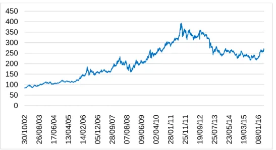
Our study covers the period from 2002 to 2016 from the Shanghai Gold Exchange. It seems that return on assets performs better in economically favorable times and gives more mediocre performances in economically unfavorable times. We plot in Figure 1 the evolution of gold prices from 2002 to 2016. From the plot, we have identified the "up-market" during the period from February 2002 to September 2011, and the “down-market” from September 2011 to May 2016. Thus, we choose to break down the whole period into two distinct phases: one phase that is favorable (up-market) and one that is unfavorable (down-market) in our study.

Figure 1. The time trend of gold prices in China 2002 to 2016 (Shanghai Gold Exchange Close Prices)

Our study covers the period from 2002 to 2016. To be able to highlight the relationship between the seasonal effects and the gold prices, we have to give an objective description of the economic trend. We chose to break down the gold prices into two distinct phases: one phase that is favorable (up-market) and one that is unfavorable (down-market). Figure 1 plots the evolution of the gold prices from 2002 to 2016. We have identified the "up-market" during the period from February 2002 to September 2011, and the “down-market” from September 2011 to May 2016.

In this article, we use the regression approach for the day of the week effect and the monthly effect by using the unobserved components model. The model to estimate the day of the week effect given by Mookerjee and Yu (1999) is as follows:

𝑅𝑡= 𝑎0+ 𝑎1𝑑1,𝑡+ 𝑎2𝑑2,𝑡+ 𝑎3𝑑3,𝑡+ 𝑎4𝑑4,𝑡+ 𝑒𝑡 , (1) 0 50 100 150 200 250 300 350 400 450 30 /10 /02 26 /08 /03 17 /06 /04 13 /04 /05 14 /02 /06 05 /12 /06 28 /09 /07 07 /08 /08 09 /06 /09 02 /04 /10 28 /01 /11 25 /11 /11 19 /09 /12 25 /07 /13 23 /05 /14 19 /03 /15 08 /01 /16

(6)

107

where 𝑅𝑡 is the return on day t and 𝑑𝑖,𝑡 is a dummy variable that takes the value of one for a

given day of the week and zero otherwise. Models 1 and 2 are basic linear models, to avoid the problem of collinearity, when the constant is included, the program (Stata Software) deletes a dummy variable. When we introduce a stochastic component in the model, these models become non-linear, we can then obtain all the variables (cf. Tables 1, 5, 6 and 7).

To test the difference between the monthly effect, Mookerjee and Yu (1999) give the following regression:

𝑅𝑡= 𝑎0+ 𝑎1𝐷𝑚𝑒+ 𝑒𝑡 , (2)

where 𝑅𝑡 is the holding period return for day t and 𝐷𝑚𝑒 is a dummy variable that takes the value

one for the first and last days of the month and takes the value of zero otherwise.

Unobserved components time series model (UCM) allows us to divide the index series into three components: an autoregressive component, a trend and a seasonal component (Harvey, 1989; Girardin and Liu, 2005).

𝐼𝑡= 𝜇𝑡+ 𝛾𝑡+ 𝜑𝑡+ 𝜀𝑡 , 𝜀𝑡 ~ 𝑁𝐼𝐷( 0, 𝜎2ε) (3)

where 𝜇𝑡, 𝛾𝑡 and φ represent autoregressive, trend and seasonal components respectively. The

trend component is simply modeled as a random walk process according to the structure of our data:

𝜇𝑡+1= 𝜇𝑡+ 𝜂𝑡, 𝜂𝑡 ~ 𝑁𝐼𝐷( 0, σ2η) , (4)

where NID (0,𝜎2) refers to a normally and independently distributed series with mean zero and

variance 𝜎2_{. For the seasonal component, we use a stochastic dummy variable seasonal model}

for the effect. All models are estimated by using the maximum likelihood approach.

4. The day of the week effect

In addition, we have analyzed the day of the week effect by using an unobserved-components time series model (UCM). We have adopted the approach of Harvey (1989) and Girardin and Liu (2005).

4.1. Whole period

The equation (1) is a general relation, but the coefficients are not significant. This finding confirms our descriptive statistics analysis in the previous section, in which we have noticed that the estimates are all significantly negative except Thursday, despite the strongly significant highest Monday return and the negative Tuesday return, the difference of level between the variables is not enough to allow us to obtain the significant day of week effect. For this reason, we have tested the variables two by two in this section.

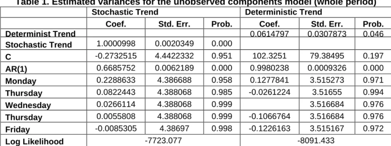
We do not find a significant day of the week effect from the series of gold prices, but it seems that the Monday return is higher than that of the other days of the week. We report results of the estimated variances of the different components of our unobserved components model in Table 1. In spite of significant coefficients, the results of regression allow us nevertheless to note the difference of level of the gold prices. The prices on Monday are higher than all other days, and we obtain the same conclusion by using the stochastic trend and the deterministic trend. However, the UCM method does not indicate a Tuesday effect. For us, it is necessary to analyze the day of the week effect by coupling the different days.

According to Table 1, results from the unobserved components model are not significant, regardless using the stochastic trend or the deterministic trend. However, we find that Monday's return is positive and Friday's return is negative.

(7)

108

Table 1. Estimated variances for the unobserved components model (whole period)

Stochastic Trend Deterministic Trend

Coef. Std. Err. Prob. Coef. Std. Err. Prob.

Determinist Trend 0.0614797 0.0307873 0.046 Stochastic Trend 1.0000998 0.0020349 0.000 C -0.2732515 4.4422332 0.951 102.3251 79.38495 0.197 AR(1) 0.6685752 0.0062189 0.000 0.9980238 0.0009326 0.000 Monday 0.2288633 4.386688 0.958 0.1277841 3.515273 0.971 Thursday 0.0822443 4.388068 0.985 -0.0261224 3.51655 0.994 Wednesday 0.0266114 4.388068 0.999 3.516684 0.976 Thursday 0.0055808 4.388068 0.999 -0.1066764 3.516684 0.976 Friday -0.0085305 4.38697 0.998 -0.1226163 3.515167 0.972 Log Likelihood -7723.077 -8091.433

Notes: Column “Stochastic Trend” presents estimations for the basic stochastic component model. In

column “Deterministic”, we introduce the deterministic component. Model 1 is a basic linear model, to avoid the problem of collinearity, when we include the constant, the program deletes a binary variable. In the right part of Table 1 (Deterministic Trend), it is a linear model, the Stata software has deleted the binary variable “Wednesday”. When we add a stochastic component in model 1, the left part of Table 1 (Stochastic Trend), it is no longer a linear model, the Stata software was able to determine the coefficients for the 5 binary variables.

Table 2 reports the day effect by coupling the days of the week. The Monday effect is significant for the whole period; returns on Mondays are always higher than that of the other days in the week in this case. Returns of Tuesdays are negative and significant. This finding confirms the result of Table 1. In fact, when we couple Monday and Tuesday together, we have a strong Monday effect. We repeat the same process, we obtain a significant Monday effect in each couple. The Monday effect is shown in the first column of the Table 2. Concerning other boxes of Table 2, we cannot distinguish any other day effect, indeed, the coefficients are not significant except Monday. This result is partly similar to what we had found for risk seekers in the previous section. By applying the mean-variance criterion, we concluded that risk seekers prefer Monday to Tuesday, Wednesday and Friday returns.

Table 2. Idiosyncratic results - Matrix of couples of the day-of-the-week effect (Whole period: 2002 – 2016)

Monday Tuesday Wednesday Thursday

Tuesday 0.0008177 (0.007)*** -0.0004198 (0.367) Wednesday 0.000116 (0.011)*** -0.0003584 (0.401) -0.0000445 (0.907) -0.0005919 (0.127) Thursday 0.0010132 (0.002)*** 0.0003844 (0.361) -0.0006359 (0.166) -0.000079 (0.838) -0.0005919 (0.127) -0.0000445 (0.907) Friday 0.0010012 (0.001)*** 0.0004106 (0.314) 0.0001253 (0.747) 0.0001854 (0.142) -0.000582 (0.145) 1.06e_-06 (0.998) 0.001253 (0.747) 0.0001854 (0.645)

Notes: In each case, the first row is the coefficient of the column of the table, and the third figure in each box is the coefficient of the row of the table. The p-value is in parentheses. For example, for the first couple Monday-Tuesday: 0.0008117 is the coefficient of Monday and the -0.0004198 is the coefficient of Tuesday; 0.007 is the p-value associated with Monday. The model of the regression is as follows:

(8)

109

Return(t) = C + αMonday + βTuesday + Return(t-1) + ɛ(t), and ɛ(t) is modeled by GARCH(1,1). *_,**_{, and}***

indicate statistical significance at the 10, 5 and 1 percent levels, respectively.

4.2. Up and down markets

We obtain similar results by using logarithm prices and by making a distinction between the up and down markets. For the up-market period, the overall pattern is similar to that observed for the whole period; the Monday returns have been positive and the Tuesday returns have been negative. However, for the down-market, returns have been negative, except for Monday returns and Friday returns.

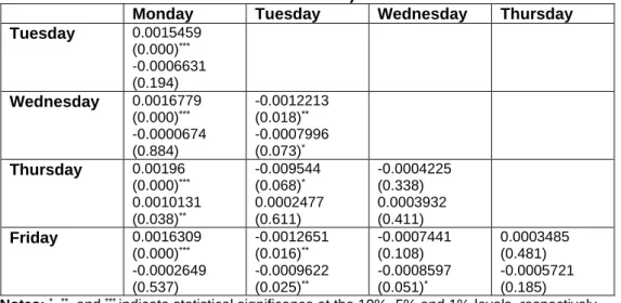
Tables 3 and 4 report results of the regression by coupling the day of the week during the up and down market. For the up-markets, when we couple Monday and any other days together, we have a strong Monday effect. Interestingly, we have detected a Tuesday effect. When we couple Tuesday with Wednesday, Thursday and Friday, we have a significant negative Tuesday effect. This effect is shown in the second column of the Table 3. Taking into account the result of regression for the up-market, it seems that there is a positive Monday effect and a negative Tuesday effect during the up-market.

Table 3. Idiosyncratic results - Matrix of couples of the day of the week effect (Up-market: 2002 – 2011)

Tuesday 0.0015459 (0.000)*** -0.0006631 (0.194) Wednesday 0.0016779 (0.000)*** -0.0000674 (0.884) -0.0012213 (0.018)** -0.0007996 (0.073)* Thursday 0.00196 (0.000)*** 0.0010131 (0.038)** -0.009544 (0.068)* 0.0002477 (0.611) -0.0004225 (0.338) 0.0003932 (0.411) Friday 0.0016309 (0.000)*** -0.0002649 (0.537) -0.0012651 (0.016)** -0.0009622 (0.025)** -0.0007441 (0.108) -0.0008597 (0.051)* 0.0003485 (0.481) -0.0005721 (0.185)

Notes: *_,**_{, and}*** _{indicate statistical significance at the 10%, 5% and 1% levels, respectively.}

Table 4. Idiosyncratic results -Matrix of couples of the day of the week effect (Down-market: 2011 – 2016)

Tuesday 0.0004278 (0.506) -0.0001618 (0.870) Wednesday 0.0002791 (0.671) -0.0006246 (0.498) -0.0004474 (0.647) -0.0008173 (0.361) Thursday 0.000802 (0.309) -0.0014778 (0.095)* -0.0013263 (0.221) -0.002122 (0.011)** -0.0009254 (0.295) -0.0011542 (0.111) Friday 0.0008049 (0.219) 0.0017386 (0.048)** 0.0001888 (0.844) 0.001615 (0.059)* -0.0003094 (0.733) 0.001476 (0.092)* -0.0014574 (0.082)* 0.0014016 (0.095)*

(9)

110

However, when we repeat the same process for the down-market (Table 4), the day of week effect is not evident. We do not find any Monday effect or Tuesday effect. Instead of the Monday effect and Tuesday effect, we obtain a Thursday effect and a Friday effect. Indeed, when we couple Friday and any other days together, we have a significant positive Friday effect. This means during the down-market period, returns on Friday are more important than other days. We noted a negative Thursday effect when we analyzed the couples Thursday-Monday and Thursday-Tuesday.

5. The monthly effect

After studying the day of the week effect, we will study the monthly effect, we start with the whole period, then we analyze the sub-periods.

5.1. Whole period

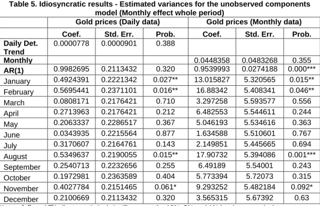
Table 5 reports the mean daily return by month during the whole period. For the whole period, we find that January and February generate the best returns. At the end of February, the price is at its highest point, so this explains the drastic decrease in March returns. The return in the middle of the year is negative, then the price begins to rise after a half-year period. This finding is available for both the up and down markets. The results obtained by analyzing the down-market period give more negative returns. This means that during unfavorable economic conditions, the decreasing price of gold continues. However, we notice that even in this condition, there are January and February effects: the price of gold decreased after the summer (September to December) then, the price increased during the period of Chinese New Year, due to more demand in the gold market.

Table 5. Idiosyncratic results - Estimated variances for the unobserved components model (Monthly effect whole period)

Gold prices (Daily data) Gold prices (Monthly data)

Daily Det. Trend 0.0000778 0.0000901 0.388 Monthly Det. Trend 0.0448358 0.0483268 0.355 AR(1) 0.9982695 0.2113432 0.320 0.9539993 0.0274188 0.000*** January 0.4924391 0.2221342 0.027** 13.015827 5.320565 0.015** February 0.5695441 0.2371101 0.016** 16.88342 5.408341 0.046** March 0.0808171 0.2176421 0.710 3.297258 5.593577 0.556 April 0.2713963 0.2176421 0.212 6.482553 5.544611 0.244 May 0.2063337 0.2286517 0.367 5.046193 5.534616 0.363 June 0.0343935 0.2215564 0.877 1.634588 5.510601 0.767 July 0.3170607 0.2164761 0.143 2.149851 5.445665 0.694 August 0.5349637 0.2190055 0.015** 17.90732 5.394086 0.001*** September 0.2540713 0.2232656 0.255 6.49189 5.54001 0.243 October 0.1972981 0.2363589 0.404 5.773394 5.72073 0.315 November 0.4027784 0.2151465 0.061* 9.293252 5.482184 0.092* December 0.2100669 0.2113432 0.320 3.565315 5.67392 0.63

Table 5 shows the results of analysis of the monthly effect by using an unobserved components time series model (UCM). In this table, we analyzed the monthly effect by using monthly prices and daily prices data. The January, February and August effect are significant,

(10)

111

this means that the prices of gold are higher than other month’s. We find the prices of June, July and December are lower than other months of the year. We can obtain similar results by using the daily returns data. This finding corroborates what we have obtained in the previous section, January, February, September and November effects are confirmed by the UCM regression.

5.2. Up and down markets

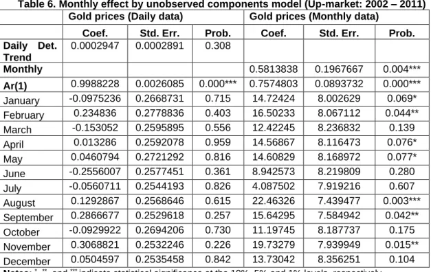
This result of UCM regression for the whole period is available for both the up and down markets. We notice that using monthly data allows us to obtain the most significant result. Table 6 and Table 7 show the seasonality in the Chinese gold market by using the UCM model for two sub periods, the monthly effect is more evident by using the monthly data between 2002 to 2016. For the day of month effect, the results are quite similar between the whole period and the up-market period, and we have more significant effect between February 2002 to September 2011. The result of monthly regression in the Table 7 indicates that the January, February, April, May, August, September and November effects are significant. The most important effect is observed in August, the effect is significant at 1% level. On the other side, the April and May effects are significant only at 10% level. This observation is logical, because during the Up-Market period, the returns are significantly positive in every January, February and November (see Table 2).

Table 6. Monthly effect by unobserved components model (Up-market: 2002 – 2011)

Daily Det. Trend 0.0002947 0.0002891 0.308 Monthly Det. Trend 0.5813838 0.1967667 0.004*** Ar(1) 0.9988228 0.0026085 0.000*** 0.7574803 0.0893732 0.000*** January -0.0975236 0.2668731 0.715 14.72424 8.002629 0.069* February 0.234836 0.2778836 0.403 16.50233 8.067112 0.044** March -0.153052 0.2595895 0.556 12.42245 8.236832 0.139 April 0.013286 0.2592078 0.959 14.56867 8.116473 0.076* May 0.0460794 0.2721292 0.816 14.60829 8.168972 0.077* June -0.2556007 0.2577451 0.361 8.942573 8.219809 0.280 July -0.0560711 0.2544193 0.826 4.087502 7.919216 0.607 August 0.1292867 0.2568646 0.615 22.46326 7.439477 0.003*** September 0.2866677 0.2529618 0.257 15.64295 7.584942 0.042** October -0.0929922 0.2694206 0.730 11.19745 8.187737 0.175 November 0.3068821 0.2532246 0.226 19.73279 7.939949 0.015** December 0.0504597 0.2535458 0.842 13.73042 8.356251 0.104

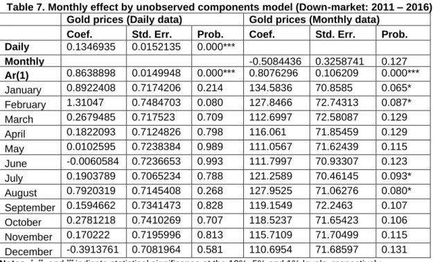
Table 7 presents the monthly effect for the period from 2011 to 2016. There are some similarities between the two sub periods, but also divergence. For example, the September and November effects are not significant, and the monthly effect (January, February, July and August effects) is significant only at 10% level. This finding corroborates the decrease trend of the gold prices during this period.

(11)

112

Table 7. Monthly effect by unobserved components model (Down-market: 2011 – 2016)

Daily Stoch. Trend 0.1346935 0.0152135 0.000*** Monthly Det. Trend -0.5084436 0.3258741 0.127 Ar(1) 0.8638898 0.0149948 0.000*** 0.8076296 0.106209 0.000*** January 0.8922408 0.7174206 0.214 134.5836 70.8585 0.065* February 1.31047 0.7484703 0.080 127.8466 72.74313 0.087* March 0.2679485 0.717523 0.709 112.6997 72.58087 0.129 April 0.1822093 0.7124826 0.798 116.061 71.85459 0.129 May 0.0102595 0.7238384 0.989 111.0567 71.62439 0.115 June -0.0060584 0.7236653 0.993 111.7997 70.93307 0.123 July 0.1903789 0.7065234 0.788 121.2589 70.46145 0.093* August 0.7920319 0.7145408 0.268 127.9525 71.06276 0.080* September 0.1594662 0.7341473 0.828 119.1549 72.2463 0.107 October 0.2781218 0.7410269 0.707 118.5237 71.65423 0.106 November 0.170222 0.7195996 0.813 115.7109 71.70499 0.115 December -0.3913761 0.7081964 0.581 110.6954 71.68597 0.131

Indeed, it is more difficult to distinguish a monthly effect during unfavorable economic conditions. In the previous section, we have noted one thing common between the whole period and the sub periods: all the negative returns are not significant while some of the positive returns are significant. The result of UCM regression corroborates this finding. In fact, by using the monthly data, the sign of the dummy variables coefficients is always positive. That means the global evolution of gold prices increases during the different periods. Taking into account the degree of the significance of the monthly variables, it seems that during the Up-Market period, the monthly effect is more important.

6. Conclusion

The Chinese Gold market is one of the emerging asset markets which offer an opportunity for international diversification. For the period from 2002 to 2016, the prices on Monday are higher than all other days, and we obtain the same conclusion by using the stochastic trend and the deterministic trend. For the up-market period, the Monday returns have been positive, and the Tuesday returns have been negative for the whole period. However, for the down-market, returns have been negative, except for Monday returns and Friday returns. For the whole period, we find that January and February generate the best returns. The return in the middle of the year is negative, then the price begins to rise after a half-year period. This finding is available for both the up and down markets. The result partially confirms the studies of Qi & Wang (2013) and Hoang et al. (2018): seasonality does exist in the Chinese Gold Market. The question to ask is: Is the Chinese Gold Market efficient? A seasonality effect during certain periods does not necessarily imply market inefficiency. On the other hand, seasonality does not mean profitability. The index may be efficient despite the regularity in price formation. To answer this question, a longer and more recent data base is needed.

(12)

113

References

Bilgin, M. H., Gozgor, G., Lau, C. K., and Sheng, X., 2018. The effects of uncertainty measures on the price of gold. International Review of Financial Analysis, 58(C), pp. 1-7.

https://doi.org/10.1016/j.irfa.2018.03.009

Bouman, S., and Jacobsen, B., 2002. The Halloween indicator, ‘Sell in May and go away’:

Another puzzle. American Economic Review, 92(5), pp. 1618-1635.

https://doi.org/10.1257/000282802762024683

Chan, K., and Chen, N., 1988. An unconditional asset pricing test and the role of firm size as an instrumental variable for risk. The Journal of Finance, 43, pp. 309-325.

https://doi.org/10.1111/j.1540-6261.1988.tb03941.x

Chan, K., and Chen, N., 1991. Structural and return characteristics of small and large firms. The

journal of finance, 46, pp. 1467-1484. https://doi.org/10.1111/j.1540-6261.1991.tb04626.x

Cross, F., 1973. The behavior of stock prices on Fridays and Mondays. Financial Analysts

Journal, 29(6), pp. 67-69.

https://doi.org/10.2469/faj.v29.n6.67

Ersan, O., and Demir, E., 2017. New season new hopes: Off-season optimism. Eurasian

Journal of Economics and Finance, 5(4), pp. 36-49.

https://doi.org/10.15604/ejef.2017.05.04.003

Fama, E. F., and French, K. R., 1992. The cross-section of expected stock return. The Journal

of Finance, 47, pp. 427-465.

https://doi.org/10.1111/j.1540-6261.1992.tb04398.x

Fama, E. F., and French, K. R., 1993. Common risk factors in the returns on stocks and bonds.

Journal of Financial Economics, 33(1), pp. 3-56. https://doi.org/10.1016/0304-405X(93)90023-5

French, K. R., 1980. Stock returns and the weekend effect. Journal of Financial Economics,

8(1), pp. 55-69. https://doi.org/10.1016/0304-405X(80)90021-5

Gibbons, M. R., and Hess, P., 1981. Day of the week effects and asset returns. The Journal of

Business, 54(4), pp. 579-596.

https://doi.org/10.1086/296147

Girardin, E., and Liu, Z., 2005. Bank credit and seasonal anomalies in China’s stock markets.

China Economic Review, 16, pp. 465-483.

https://doi.org/10.1016/j.chieco.2005.03.001

Gultekin, M. N., and Gultekin, N., 1983. Stcok market seasonality: Internatinal Evidence. Journal

of Financial Economics, 12(4), pp. 469-481. https://doi.org/10.1016/0304-405X(83)90044-2

Guo, B., Luo, X., and Zhang, Z., 2014. Sell in may and go away: Evidence from China. Finance

Research Letters, 11, pp. 362-368. https://doi.org/10.1016/j.frl.2014.10.001

Harvey, A. C., 1989. Forecasting structural time series models and the Kalman filter.

Cambridge: Cambridge University Press.

https://doi.org/10.1017/CBO9781107049994

Hoang, T.-H.-V., Wong, W.-K., Xiao, B., and Zhu, Z., 2018. The seasonality of gold prices in China: Does the risk-aversion level matter? Accounting and Finance, 09 September

2018. https://doi.org/10.1111/acfi.12396

Jacobsen, B., and Bouman, S., 2002. The Halloween indicator, 'Sell in may and go away':

Another puzzle. American Economic Review, 92(5), pp. 1618-1635.

https://doi.org/10.1257/000282802762024683

Jacobsen, B., and Zhang, C., 2012. The Halloween indicator: Everywhere and all the time.

Working paper. Massey University.

https://doi.org/10.2139/ssrn.2154873

Kaiser, L., 2019. Seasonality in cryptocurrencies. Finance Research Letters, 31(C), pp. 232-238.

https://doi.org/10.1016/j.frl.2018.11.007

Keim, D., 1983. Size-related anomalies and stock return seasonality: Further empirical

evidence. Journal of Financial Economics, 12(1), pp. 13-32.

https://doi.org/10.1016/0304-405X(83)90025-9

Kim, M. K., and Burnie, D. A., 2002. The firm size effect and the economic cycle. The Journal of

Financial Research, 25(1),pp. 111-124.

https://doi.org/10.1111/1475-6803.00007

Long, H., Zaremba, A., Demir, E., Szczygielski, J., and Vasenin, M., 2020. Seasonality in the cross-section of cryptocurrency returns. Finance Research Letters. In press.

(13)

114

Mitchell, J. D., and Ong, L. L., 2006. Seasonalities in China's stock markets: Cultural or

structural? IMF working paper, 96/4.

https://doi.org/10.5089/9781451862645.001

Mookerjee, R., and Yu, Q., 1999. Seasonality in returns on the Chinese stock markets: The case of Shanghai and Shenzhen. Global Finance Journal, 10(1), pp. 93-105.

https://doi.org/10.1016/S1044-0283(99)00008-3

Qi, M., and Wang, W., 2013. The monthly effects in Chinese gold market. International

Journalof Economics and Finance, 5(10), pp. 141–146.

https://doi.org/10.5539/ijef.v5n10p141

Reinganum, M. R., 1999. The significance of market capitalization in portfolio management over

time. Journal of Portfolio Management, 25(4), pp. 39-50.

https://doi.org/10.3905/jpm.1999.319750

Ritter, J. R., 1978. An explanation of the rurn of the year effect. Graduate School of Business

Administration Working paper. University of Michigan.

Rogalski, R. J., 1984. New findings regarding day-of-the-week returns over trading and

non-trading periods: A note. Journal of Finance, 39(5), pp. 1603-1614.

https://doi.org/10.1111/j.1540-6261.1984.tb04927.x

Roll, R., 1977. A critique of the asset pricing theory tests. Journal of Financial Economics, 4(2),

pp. 129-176.

https://doi.org/10.1016/0304-405X(77)90009-5

Schwert, G. W., 2003. Anomalies and market efficiency. In: G. M., Constantinides, M. Harris, and R. M Stulz, eds. 2003. Handbook of the economics of finance. Amsterdam:

Elsevier. pp. 937-972. https://doi.org/10.1016/S1574-0102(03)01024-0

Xiao, B., 2016. The monthly effect and the day of week effect in the American stock market.

International Journal of Financial Research, 7(2), pp. 11-17.

https://doi.org/10.5430/ijfr.v7n2p11

View publication stats View publication stats