HAL Id: cel-00392214
https://cel.archives-ouvertes.fr/cel-00392214
Submitted on 5 Jun 2009
HAL is a multi-disciplinary open access
archive for the deposit and dissemination of sci-entific research documents, whether they are pub-lished or not. The documents may come from teaching and research institutions in France or abroad, or from public or private research centers.
L’archive ouverte pluridisciplinaire HAL, est destinée au dépôt et à la diffusion de documents scientifiques de niveau recherche, publiés ou non, émanant des établissements d’enseignement et de recherche français ou étrangers, des laboratoires publics ou privés.
Introduction to Numerical Methods in Probability for
Finance
Gilles Pagès
To cite this version:
Gilles Pagès. Introduction to Numerical Methods in Probability for Finance. 3rd cycle. Hanoi (Vietnam), 2007, pp.71. �cel-00392214�
Introduction to Numerical Methods in Probability for
Finance
—–
School Mathematical Finance - Hanoi 2007
—–
CIMPA
—–
Gilles Pag`
es
LPMA-Universit´e Paris 6 — E-mail: [email protected] — http: //www.proba.jussieu.fr/pageperso/pages 25.04.2007Useful links
✄The website of the Master 2 Probabilit´e & Finance (Univ. Pierre & Marie Curie, Paris, France): www.masterfinance.proba.jussieu.fr
✄A website devoted to Quantitative Finance:
www.maths-fi.com/uk default.asp
1
Simulation of random variables
1.1 Pseudo-random numbers
From a mathematical point of view, the definition of a sequence of (uniformly distributed) random numbers (over the unit interval [0, 1]) should be :
“Definition.” A sequence xn, n≥ 1, of [0, 1]-valued real numbers is a sequence of random numbers
if there exists a probability space (Ω,A,P), a sequence Un, n ≥ 1, of i.i.d. random variables with
uniform distribution U([0, 1]) and ω ∈ Ω such that xn= Un(ω) fo every n≥ 1.
But this naive and abstract definition is not satisfactory because the “scenario” ω ∈ Ω is may be not a “good” one i.e. not a “generic” . . . ? Many probabilistic properties (like the law of large numbers to quote the most basic one) are only satisfied P-a.s.. Thus, if ω precisely lies in the
negligible set that does not satisfy one of them.
Whatever, one usually cannot have access to an i.i.d. sequence of random variables (Un) with
distributionU([0, 1])! Any physical device would too slow and not reliable. Some works by logicians like Martin-L¨of lead to consider that a sequence (xn) that can be generated by an algorithm cannot
be considered as “random” one. Thus the digits of π are not random in that sense. This is quite embarrassing since an essential requested feature for such sequences is to be generated almost instantly on a computer!
The approach coming for computer and algorithmic sciences is not really more tractable since their definition of a sequence of random numbers is that the complexity of the algorithm to generate the first n terms behaves like O(n). The rapidly growing need of good (pseudo-)random sequences with the explosion of Monte Carlo simulation in many fields of Science and Technology (I mean not only neutronics) after World War II lead to adopt a more pragmatic approach – say – heuristic – based on a statistical tests. The idea is to submit some sequences to statistical tests (uniform distribution, block non correlation, rank tests, etc)
For practical implementation, such sequences are finite , as is the accuracy of computers. One considers some sequences (xn) of so-called pseudo-random numbers displaying as
xn=
yn
N, yn∈ {0, . . . , N − 1}.
One classical process is to generate the yn by a congruential induction :
yn+1≡ ayn+ b mod. N
where gcd(a, N ) = 1, so that a is invertible in the multiplicative group ((Z/NZ)∗,×) (invertible
elements of Z/NZfor the product).
If b = 0 (the most common case), one speaks of homogenous generator.
One will choose N as large as possible given the computation capacity of the computers (with integers) (N = 231−1 for a 32 bits architecture, etc).
Still if b = 0, the length of the sequence will be settled by the period τ := min{t / at ≡
1 mod. N} of a in ((Z/NZ)∗, +).
Since card(Z/NZ)∗= ϕ(N ) where ϕ(N ) := card{1 ≤ k ≤ N −1, tq pgcd(k, N) = 1} is the Euler
function, it follows from Lagrange theorem that:
(where <a> := multiplicative sub-group of (Z/NZ)∗ generated by a). Let us recall ϕ(N ) = N Y p|N, pprime µ 1−1 p ¶ .
The (difficult) study of ((Z/NZ)∗,×) when N is a primary integer leads to the following theorem: Theorem 1 Let N = pα, p prime, α∈N∗.
(a) If α = 1 (i.e. N = p prime), then ((Z/NZ)∗,×) (whose cardinality is p − 1) is a cyclic group.
This means that there exists a∈ {1, . . . , p − 1} s.t. (Z/pZ)∗ =<a>. Hence the maximal period is
τ = p− 1.
(b) If p = 2, α≥ 3, (Z/NZ)∗, (whose cardinality is 2α−1 = N
2), is not cyclic. The maximal period is then τ = 2α−2 with a≡ ±3 mod. 8.
(c) If p6= 2, then (Z/NZ)∗, (whose cardinality is pα−1(p− 1)), is cyclic, hence τ = pα−1(p− 1).
It is generated by any element a whose class ˜a in (Z/pZ) spans the cyclic group ((Z/pZ)∗,×).
However, one should be aware that the length of a sequence, if it is a necessary asset of a sequence, provides no guarantee or even clue that a sequence is a good as a sequence of pseudo-random numbers! Thus, the generator of the FORTRAN IMSL library does not fit in the formerly described setting: one sets N := 231− 1 (which is a prime number), a := 75, b := 0 (a6≡0 mod.8).
Another approach to random number generation is based on shift register and relies upon the theory of finite fields.
1.2 The fundamental principle of simulation
Theorem 2 Let (E, d) be a Polish space (complete and separable) and X : (Ω,A,P) → (E, ) be a
random variable with distributionP
X. Then there exists a Borel function ϕ : ([0, 1],B([0, 1]), λ[0,1])→
(E,Bor(E), PX) such that
P
X = λ◦ ϕ−1
where λ◦ ϕ−1denotes the image of the Lebesgue measure λ
[0,1] by ϕ.
As a consequence this means that, if U denotes a uniformly distributed random variable on a probability space, then
X= ϕ(U ).d
The interpretation is that any E-valued random variable can be simulated from a uniform distribution. In practice this turns out to be a purely theoretical result which is of no help for practical simulation.
1.3 The distribution function method
Let µ be a probability distribution on (R,B(R)) having a continuous increasing distribution function
F . Then F has an inverse function F−1 defined (0, 1).
Proposition 1 If L(U) = U((0, 1)), then X := F−1(U )= µ.d
Proof. : Let x∈R,P(X ≤ x) =P(F−1(U )≤ x). Now F−1 is increasing, hence{F−1(U )≤ x} =
Remark. • If µ has a probability density f satisfying {f = 0} has an empty interior, then F (x) =
Z x −∞
f (u)du is continuous, increasing. • One can replace Rby any interval [a, b]⊂R.
• When F is simply non-decreasing (or discontinuous at some points), one defines the canonical right continuous inverse Fr−1 by:
∀u ∈ (0, 1), Fr−1(u) = inf{s/F (s) ≥ u}.
One shows that Fr−1 is non-decreasing, right continuous and
Fr−1(u)≤ x ⇒ F (x) ≥ u et F (x) > u ⇒ Fr−1(u)≤ x. Hence X = Fd r−1(U ) since P(X≤ x) =P(Fr−1(U )≤ x) ( ≤P(F (x)≥ U) = F (x) ≥P(F (x) > U ) = F (x) ) = F (x). If X takes finitely many values in a R, on retrieves the standard simulation method.
• One could have considered the left continuous inverse defined by ∀u ∈ (0, 1), Fl−1(u) = inf{s/F (s) > u}.
with the same result.
Examples : • Simulation of an exponential distribution. Let X =d E(λ), λ > 0. Then
∀ x∈ (0, ∞), FX(x) = λ
Z x
0 e
−λξdξ = 1− e−λx.
Consequently, for every y ∈ (0, 1), F−1(u) = − log(1 − u)/λ. Now, using that U = 1d − U if
U = U ((0, 1)) yieldsd
X =− log(U)/λ=d E(λ). • Simulation of a Cauchy(c), c > 0, distribution.
We know that PX(dx) = c π(x2+ c2)dx. ∀x ∈R, FX(x) = Z x −∞ c u2+ c2 du π = 1 π µ Arctan(x c) + π 2 ¶ , hence FX−1(x) = c tan(π(u− 1/2)). It follows that
X = c tan(π(U− 1/2))= Cauchy(c).d • Simulation of a Pareto(θ), θ > 0, distribution.
We know that PX(dx) = θ
x1+θ1{x≥1}dx. FX(x) = 1− x−θ so that
• Simulation of a purely discrete distribution supported by E ⊂R.
Let E :={x1, . . . , xN} and X : (Ω, A,P)→ E an E-valued r.v. with distribution P(X = xk) =
pk, 1≤ k ≤ N. Then, one checks that
∀u∈ (0, 1), FX−1(u) = N X k=1 xk1{p1+···+pk−1<u≤p1+···+pk} so that X =d N X k=1 xk1{p1+···+pk−1<U ≤p1+···+pk}.
The yield of the procedure is ¯r = 1 but when implemented naively its complexity – which corre-sponds to (at most) N comparisons for every simulation – may be quite high. See [17] for some considerations (in the spirit of quick sort algorithms) which lead to a O(log N ) complexity. Fur-thermore, this procedure underlines that the pk are known (as real numbers) which is not always
the case even in a priori simple situations
• Simulation of a Bernoulli random variable B(p), p∈ (0, 1). This is the simplest application of the previous method since
X = 1{U≤p}= B(p).d The yield of the method is 1.
• Simulation of a Binomial random variable B(n, p), p∈ (0, 1), ≥1.
One relies on the very definition of the binomial distribution as the law of the sum of n inde-pendent B(p)-distributed random variables i.e.
X =
n
X
k=1
1{Uk≤p}= B(n, p).d
where (U1, . . . , Un) are i.i.d. B(p)-distributed r.v. Note that this procedure has a very bad yield,
namely n1 and needs n comparisons like the standard method (without any shortcut). Its asset is that it does not require the computation of the probabilities pk’s.
1.4 The rejection method (Von Neumann)
Let f, g : (Rd,B(Rd))−→ R+ be two probability densities with respect to a nonnegative measure
µ on (Rd,B(Rd)). Assume g > 0 µ-a.s. and
∀ x∈Rd, f (x)≤ cg(x).
Proposition 2 Let (Un, Yn)n≥1 be a sequence of i.i.d. r.v. with distribution U ([0, 1])⊗PY
(inde-pendent marginals) defined on (Ω,A,P). Assume PY(dy) = g(y)µ(dy)
Let
τ := min{k ≥ 1 | c Ukg(Yk) < f (Yk)}.
Then, τ has a geometric distribution G∗(p) with parameter p :=P(c U1g(Y1) < f (Y1))) and
In practice, one needs
– to simulate the distribution of Y , – to compute the functions f and g, ms on a computer at a reasonable cost.
The yield of the method is obviously 1τ and its mean yield
E1
τ =− p
1− plogp.
Proof. Step 1: Let ϕ :Rd→R be a bounded Borel test function. By Fubini’s Theorem,
E³ϕ(Y )1 {c Ug(Y )≤f(Y )} ´ = Z Rdϕ(y) Z 1 0 1{cug(y)≤f(y)}g(y)µ(dy) = Z Rdϕ(y) Z 1 0 1{cug(y)≤f(y)}∩{g(y)>0}g(y)µ(dy) = Z Rdϕ(y) Z 1 0 1{u≤ f(y) cg(y)}∩{g(y)>0} g(y)µ(dy) = Z {g(y)>0} ϕ(y)f (y) cg(y)g(y)µ(dy) = c Z Rdϕ(y)f (y)µ(dy).
If ϕ≡ 1, then c =P(U f (Y )≤ cg(Y )), hence, elementary conditioning yields E(ϕ(Y )|{c Ug(Y ) ≤ f(Y )}) =
Z
Rdϕ(y)f (y)µ(dy)
i.e.
L (Y |{c Ug(Y ) ≤ f(Y )}) = f(y)µ(dy). Step 2: Let B∈ B(Rd). Then
P(X ∈ B) = X n≥1 E³1 {τ=n}1{Yn∈B} ´ = X n≥1
P({c U1g(Y1)≥ f(Y1)})n−1P({c U1g(Y1) < f (Y ), Y1 ∈ B})
where we used that the sequence (Un, Yn)n≥1 is i.i.d.. Hence
P(X ∈ B) = X n≥1 E³1 {τ=n}1{Yn∈B} ´ = X n≥1
P({c U1g(Y1)≥ f(Y1)})n−1P({c Ug(Y ) < f(Y1), Y1∈ B})
= P(Y ∈ B | c U1g(Y1)≤ f(Y1)).
Combining this with Step 1 yieldsP
Corollary 1 Set by induction for every n≥ 1
τ1 := min{k ≥ 1 | c Ukg(Yk) < f (Yk)} and τn+1:= min{k ≥ τn+ 1| c Ukg(Yk) < f (Yk)}.
then the sequence
Xn:= Yτn
is an i.i.d. P
X-distributed sequence of r.v.
The easy proof is left to the reader
Remark. The average yield of the rejection method is defined by ¯r :=P(c U1g(Y1)≤ f(Y1)): this
means that in average one needs to simulate 1r¯ to obtain onePX-distributed number.
Applications. ✄ Uniform distributions on bounded domains D. Let D⊂ [−M, M]d, λ
d(D) > 0
and let Y = U ([d −M, M]d) and τ := min{n | Y
n∈ D}. Then,
Xτ = U (D).d
This follows (exercise) from the above proposition with
g(u) := (2M )−d1[−M,M]d(y).λd(dy)
| {z } µ(dy) and f (x) = 1 λd(D) 1D(x)λd(dx)≤ (2M )d λd(D) g(x).
A standard application is to consider the unit ball of Rd, D := Bd(0; 1). When d = 2, this is
involved in the so-called polar method, see below, for the simulation of N (0; I2) random vectors.
✄The γ(α)-distribution Let α > 0 andP
X(dx) = fα(x)λ(dx) where
fα(x) = 1
Γ(α)x
α−1e−x1
(0,+∞)(x).
(Keep in mind Γ(a) =R0+∞ua−1e−udu). Note that when α = 1 the gamma distribution is but the exponential distribution.
– If 0 < α < 1, one uses the rejection method, based on the probability density gα(x) = αe
α + e
³
xα−11{0<x<1}+ e−x1{x≥1}´. First, one checks that fα(x)≤ cαgα(x) where
cα =
α + e αeΓ(α).
Then, one uses the inverse distribution function to simulate the random variable with distribution
P
Y(dy) = gα(y)λ(dy). Namely, if Gα denotes the distribution function of Y , one checks that, for
every u∈ (0, 1), G−1α (u) = µα + e e u ¶1 a 1{u< e α+e}− log µ (1− u)α + e αe ¶ 1{u≥ e α+e}
– If α ≥ 1, Then X = X′ + X′′, with X′ and X′′ are independent and X′ has a gamma
distribution with parameter [α] and X” has a gamma distribution with parameter{α} = α − [α]. Consequently one may assume that α = n∈N. Then,
X = ξ1+· · · + ξn
where ξk are i.i.d. with exponential distribution. Consequently, if U1, . . . , Un are i.i.d. uniformly
distributed random variables
X= logd à n Y k=1 Uk ! .
1.5 The Box-M¨uller method for normal vectors
1.5.1 d-dimensional Normal vectors
One relies on the Box-M¨uller method, which is probably the most efficient method to simulate couples of bi-variate normal distributions.
Proposition 3 Let R2 et Θ : (Ω,A,P) → R be two independent r.v. with distributions L(R2) =
E(12) and L(Θ) = U([0, 2π]) respectively. Then
X := (R cos Θ, R sin Θ)=d N (0, I2)
where R :=√R2.
Proof. : Let f be a bounded Borel function.
Z Z R2f (x1, x2)exp(− x2 1+ x22 2 ) dx1dx2 2π = Z Z
f (ρ cos θ, ρ sin θ)e−ρ22 1R∗
+(ρ)1]0,2π[(θ)ρ
dρdθ 2π using the standard change of variable: x1 = ρ cos θ, x2= ρ sin θ. Setting now ρ =√r, one has:
Z Z R2f (x1, x2)exp(− x21+ x22 2 ) dx1dx2 2π = Z Z f (√r cos θ,√r sin θ)e −r 2 2 1R+∗(ρ)1]0,2π[(θ) drdθ 2π = IE³f (√R2cos Θ,√R2sin Θ)´= IE(f (X)).
♦
Corollary 2 One can simulate a distribution N (0; I2) from a couple (U1, U2) of independent r.v.
with distribution U ([0, 1]) by setting
X :=µq−2 log(U1) cos(2πU2),
q
−2 log(U1) sin(2πU2)
. The yield of the simulation is ρ = 1.
Proof. Simulate the exponential distribution using the inverse distribution function and note that if U ∼ U([0, 1]), then L(2πU) = U([0, 2π]). ♦
To simulate a d-dimensional vectorN (0; Id), one may assume that d is even and “concatenate”
the above process using a d-tuple (U1, . . . , Ud) of i.i.d. U ([0, 1]) r.v..
Exercise (Polar method) Let (U1, U2)= U (B(0; 1)). Setd
X := (U1 q −2 log(R2)/R2, U 2 q −2 log(R2)/R2).
Show that X =d N (0; I2). Derive a simulation method forN (0; I2) combining the above identity
1.5.2 d-dimensional Gaussian vectors (with general covariance matrix)
Let Σ be a covariance matrix and X =d N (0; Σ). Σ is a symmetric nonnegative so there exists a unique symmetric nonnegative matrix commuting with Σ, denoted √Σ such that √Σ2 = Σ. A straightforward computation shows that if
Z =d N (0; Id) then
√
ΣZ =d N (0; Σ)
One can compute√Σ by diagonalizing Σ in the orthogonal group: since if Σ = P∗Diag(λ1, . . . , λd)P
then √Σ = P∗Diag(√λ1, . . . ,√λd)P where P stands for the transpose of the orthogonal matrix
P .
However, one will prefer usually rely on the Cholevsky method (see e.g. Numerical Recipes [37] by decomposing
Σ = T T∗ where T is an lower triangular matrix. Then
T Z=d N (0; Σ).
1.6 Vanilla options pricing in a Black-Scholes model by Monte Carlo 1.7 Premium computation
For the sake of simplicity, one considers a 2-dimensional correlated Black-Scholes model (under its unique risk neutral probability)but a general d-dimensional can be defined likewise.
dXt0 = rXt0dt, X00= 1,
dXt1 = Xt1(rdt + σ1Wt1), X01= x10,
dX2
t = Xt2(rdt + σ1Wt2), X02= x20,
with the usual notations (r interest rate, σ1, σ2 volatility. In particular, W = (W1, W2) denotes a
correlated bi-dimensional Brownian motion such that < W1, W2>
t= ρ dt. The filtration F is the
augmented filtration of W . Then, for every t∈ [0, T ]
Xt0 = ert X1 t = x10e(r− σ21 2 )t+σ1Wt1, Xt2 = x20e(r− σ22 2 )t+σ2Wt2.
A European vanilla option with maturity T > 0 is an option related to a European payoff hT := h(XT)
which only depends on X at time T . In such a complete market the option premium at time 0 is given by
V0 = e−rTE(h(XT))
and more generally at any time t∈ [0, T ]
Vt= e−r(T −t)E(h(XT)|Ft).
The fact that W has independent stationary increments implies that X1 and X2 have
indepen-dent stationary ratios so that if
then Vt = e−r(T −t)E(h(XT)|Xt) = e−r(T −t)E h à XTi Xi t × Xti ! i=1,2 |St = e−r(T −t)E(h((xiX i T −t Xi 0 )i=1,2)xi=Xi t = v(Xt, T − t).
Examples. • Vanilla call: h(x1, x2) = (x1− K)
+. There is a closed form for this option which is
but the celebrated Black-Scholes formula
CallBS0 = C(x0, K, T, r, σ) = s0Φ0(d1)− e−rTKΦ0(d2) with d1 = log(x10/K) + (r + σ21 2 )T σ1 √ T , d2= d1− σ1 √ T . (Φ0 denotes the distribution function of theN (0; 1)-distribution.
• Best of call with strike price K:
hT = (max(X
1
T, X
2
T)− K)+.
A quasi-closed form is available involving the distribution function of the bi-variate (correlated) normal distribution. It may be interesting to price it by MC (although P DE is also quite appro-priate).
• Exchange Call Spread:
hT = ((X
1
T − X
2
T)− K)+.
For this payoff no closed form is available. One has the choice between a PDE approach (quite appropriate in this 2-dimensional setting) and a Monte Carlo simulation.
We will illustrate on this last example the regular Monte Carlo procedure.
Pricing by Monte Carlo : the regular procedure A crude Monte Carlo amounts to writing e−rThT d = ϕ(Z1, Z2) := Ã s10exp (σ 2 1 2 T + σ1 √ T Z1)− s20exp− σ22 2 T + σ2 √ T Z2)− Ke−rT ! +
where Z = (Z1, Z2) =d N (0; I2) (the dependence of ϕ in xi0, etc is dropped). Then, simulating a
M -sample (Zm)1≤m≤M of theN (0; I2) distribution using e.g. the Box-M¨uller yields the estimate
ExchSpread0 = e−rTE((XT1 − X 2 T)− K)+) =E(ϕ(Z 1, Z2))≈ ϕ M := 1 M M X m=1 ϕ(Zm).
One computes an estimate for the variance using the same sample VM(ϕ) = 1 M − 1 M X k=1 ϕ(Zm)2− M M− 1(ϕM) 2 ≈ Var(ϕ(Z))
since M is large enough. Then one designs a confidence interval for Eϕ(Z) at level α∈ (0, 1) by setting IM = ϕM − aα s VM(ϕ) M , ϕM + aα s VM(ϕ) M
where aα is defined byP(|N (0; 1)| ≤ aα) = α (or equivalently 2Φ0(aα)− 1 = α. Some
approxima-tions are hidden in what precedes from a statistical viewpoint, in particular the fact that ϕpM−Eϕ(Z)
VM(ϕ)
does have a normal distribution, which is in fact only true asymptotically. However, within the usual range of simulation implemented for numerical purpose, this approximation is quite satisfactory, in fact more satisfactory than in many statistical applications where it is usually made.
1.8 Greeks (sensitivity to the option parameters: the elementary approach)
The greeks or sensitivities denote the set of parameters obtained as derivatives of the premium of an option with respect to some of its parameters: the starting value, the volatility, etc. In many reasonably elementary situations, one simply needs to apply some more or less standard theorem like
Theorem 3 (Inverting differentiation and expectation) (a) Let Ψ : I × (Ω, A,P) → R where I
denotes a nonempty interval of R. Let x
∞∈ I. If the function Ψ satisfies
(i) for every x∈ I, the r.v. Ψ(ξ, .)∈ L1
R(P),
(ii) P(dω)-a.s., ∂Ψ
∂x(x∞, ω) exists,
(iii) There exists Y ∈ L1R+(P) such that for every x∈ I, P(dω)-a.s. |Ψ(x, ω) − Ψ(u
∞, ω)| ≤ Y (ω)|x − x∞|,
then, the function ψ(x) :=E(Ψ(x, .)) is defined at every ξ∈ I, differentiable at x
∞ with derivative ψ′(x∞) =E µ∂Ψ ∂x(x∞, .) ¶ . (b) If Ψ satisfies (i) and
(ii)glob P(dω)-a.s.,
∂Ψ
∂x(x, ω) exists at every x∈ I,
(iii)glob There exists Y∈ L1R+(P) such that for every x∈ I,
P(dω)-a.s. ¯ ¯ ¯ ¯ ∂Ψ(x, ω) ∂x ¯ ¯ ¯ ¯≤ Y (ω),
then, the function ψ(x) :=E(Ψ(x, .)) is defined and differentiable at every ξ∈ I, with derivative
ψ′(x) =E
µ∂Ψ
∂x(x, .)
.
Remarks. • This is a special case of a general result of Integration theory and one can replace the probability space (Ω,A,P) by any measured space (E,E, µ).
• Some variants of the result can be established to get a theorem for differentiability of functions defined onRd or for holomorphic functions, etc.
1.8.1 Working with the random process
To illustrate the different methods to compute the sensitivity, we will consider the 1-dimensional case of the Black-Scholes and temporarily change our notation by setting
dXtx = Xtx(rdt + σdWt), X0x= x > 0
so that Xtx = x exp ((r−σ2
2 )t + σWt). Then we consider, for every x∈ (0, ∞),
f (x) =E(ϕ(Xx
T)),
where ϕ : (0, +∞) →Ris in L1(P Xx
T). We will first work on the scenarii space (Ω,A,
P), because
this approach contains the seed of methods that can be developed in much more general settings in which the SDE has no explicit solution like in the Black-Scholes model. However, as soon as a closed form is available for the density of Xx
T, it is more efficient to use the next paragraph.
Proposition 4 (a) If ϕ is differentiable with polynomial growth, then f is differentiable and
f′(x) =E µ ϕ′(XTx)X x T x ¶ .
(b) If ϕ is simply Borel function with polynomial growth, then f is still differentiable and f′(x) =E µ ϕ(XTx)WT xσT ¶ .
Proof. (a) This straightforwardly follows from the explicit expression for XTx and the above differentiation Theorem 3.
(b) Now, still under the assumption (a) (with µ := r−σ22), f′(x) =
Z
R
ϕ′(x exp (µT + σ√T u)) exp (µT + σ√T u)−u
2 2 du √ 2π = Z R ∂ϕ(x exp (µT + σ√T u)) ∂u exp (−u2/2) xσ√T du √ 2π = Z R
ϕ(x exp (µT + σ√T u))uexp (−u
2/2)
xσ√T
du √
2π
where we used an integration by part in the last line. Finally, coming back to Ω, f′(x) = 1 xσTE ³ ϕ(XTx)WT ´ . (1.1)
When ϕ is not differentiable, let us sketch the extension by density when ϕ has compact support. Then ϕ can be approximated in every Lp(P) by differentiable functions ϕn with compact support
(use a mollifier and a convolution approximation). Then, with obvious notations, fn′(x) converges uniformly on compact sets of (0,∞) to f′(x) defined by (1.1). Furthermore fn(x) converges toward
f (x). Consequently f is differentiable with derivative f′.
Remark. Using item (a) of Theorem 3 and the fact that P(Xx = y) = 0 for every y > 0, one
derives that claim (a) in the proposition may remain true if ϕ is not differentiable at countably many points. This extends e.g. the first formula to the case of functions ϕ(x) = (x− K)+ or (K− x)+.
✄Exercise: Application to the computation of the γ. As a result f ”(x) := 1
x2σTE
³
ϕ′(XTx)WTXTx− ϕ(XTx)WT´ if ϕ is differentiable with a derivative having linear growth, and
f ”(x) := 1 x2σTE Ã ϕ(XTx) Ã WT2 σT − WT − 1 σ !! . if ϕ is simply Borel with linear growth.
✄ Computation of the vega. One shows likewise the expression for the vega i.e. the derivative of the premium with respect to the volatility parameter σ under the same assumptions on ϕ, namely
∂ ∂σE(ϕ(X x T)) =E ³ ϕ′(XTx)(WT − σT )X x T ´ = 1 σTE ³ ϕ(XTx)WT ´
if ϕ is differentiable with a derivative with polynomial growth. An integration by part then shows that ∂ ∂σE(ϕ(X x T) =E Ã ϕ(XTx) Ã W2 T σT − WT − 1 σ !! .
1.8.2 A direct approach based on differentiation on the state space
In fact, one can also carry on the computations directly on the state space of the process without specifying the Black-Scholes model provided the solution at time t, Xtx, has an explicit probability density pt(x, y)µ(dy) with respect to a reference measure µ on the real line. If θ denotes a real
parameter of interest of the structure equation that defines Xx (which may turn to be x itself),
one has at least formally
f (θ) =E(ϕ(Xx T)) = Z R ϕ(y)pT(θ, x, y)µ(dy) so that f′(θ) = Z R ϕ(y)∂pT ∂θ (θ, x, y)µ(dy) = Z R ϕ(y) ∂pT ∂θ pt(θ, x, y) (θ, x, y)pT(θ, x, y)µ(dy) = E µ ϕ(XTx)∂ log(pT) ∂θ (θ, x, X x T) ¶ (1.2)
Of course, the above computations need to be supported by appropriate assumptions (domina-tion, etc).
Exercise (a) Compute the probability density pT(x, y) of XTx.
(b) Re-establish all the above formulae using this approach.
A multi-dimensional version of this result can be established the same way round. However, this straightforward and simple approach to “greek” computation remains marginal outside the Black-Scholes world since it needs to have access to an explicit form for the probability density of the asset at time T . When dealing with path-dependent options (or even worse American options), this approach already fails even in a Black-Scholes model.
This is why we are lead to “go back” on the “scenarii” space Ω. Then, some extensions of the first approach are possible: if the function and the diffusion coefficients (when the risky asset prices follow a Brownian diffusion) are smooth enough, one usually relies on the so-called tangent process. A more sophisticate method is to introduce some Malliavin calculus methods which correspond to a differentiation theory with respect to the generic Brownian paths. This second topic is beyond the scope of the present course.
1.8.3 The tangent process method
In fact if the coefficients of the SDE are regular enough, one can differentiate directly the processes with respect to a given parameter. We refer to section 4.
2
Variance reduction
2.1 Static control variate
Let X, X′∈ L2
R(Ω,A,P) satisfying
EX =EX′= m∈R, Var(X), Var(X′), Var(X− X′) > 0
✄The parameter m is to be computed by a Monte Carlo simulation. Let Xk, k≥ 1 be a sequence of i.i.d. copies of X. Then (SLLN )
m = lim M →∞XM P-a.s., with XM := 1 M M X k=1 Xk
with a convergence ruled by the Central Limit Theorem (CLT ) √ M³XM− m ´ L −→ N (0; Var(X)) as M → ∞. so that P µ m∈ · XM − a σ(X) √ M , XM + a σ(X) √ M ¸¶ ≈ 2Φ0(a)− 1.
where σ(X) :=pVar(X) and Φ0(x) =R−∞x e−
ξ2
2 √dξ
2π.
✄Question: Which random vector (distribution. . . ) is more appropriate?
A natural answer is : if both X and X′ can be simulated with an equivalent cost (complexity), then the one with the lowest variance is the best choice i.e.
X if Var(X) < Var(X′), X′ otherwise. provided this is known a priori.
✄ Practical implementation. Usually, the problem appears as follows: there exists a random variable Ξ∈ L2
R(Ω,A,P) such that
(i) EΞ can be computed at a very low cost by a deterministic method (closed form, numerical
analysis method)
(iii) the variance Var(X− Ξ) < Var(X). Then, the random variable
X′= X− Ξ +EΞ
can be simulated at the same cost as X,EX′ =EX and Var(X′) < Var(X).
✄In option pricing the payoffs are usually nonnegative. In that case, any r.v. Ξ satisfying (i)-(ii) and
0≤ Ξ ≤ X
can be considered as a good candidate to reduce the variance, especially if Ξ is not too far from X in some way. However, note that it does not imply (iii) (if X ≡ 1, then Var(X) = 0 whereas a uniformly distributed random variable Ξ on [1− η, 1] has clearly a nonzero variance. . . ).
2.1.1 Jensen inequality and variance reduction
Jensen inequality is an efficient tool to design control variate when dealing with path-dependent exotic option pricing as illustrated by the following examples:
Examples: • Asian options and Kemna-Vorst control variate in a Black-Scholes dynamics (see [29]) Let hT = ϕ³T1 R0T Xx
tdt
´
where ϕ is nonnegative and non-decreasing and Xtx = x exp ((r−σ
2
2 )t + σWt), x > 0
is a Black-Scholes dynamics with volatility σ and interest rate r. Then, Jensen inequality applied to the probability measure T11[0,T ](t)dt implies
1 T Z T 0 Xtxdt ≥ x exp à 1 T Z T 0 (r− σ2/2)t + σWt)dt ! = x exp à 1 2(r− σ 2/2)T + σ T Z T 0 Wtdt) ! . Now Z T 0 Wtdt = T WT − Z T 0 sdWs= Z T 0 (T − s)dWs so that 1 T Z T 0 Wtdt d =N à 0; 1 T2 Z T 0 s 2ds ! =N µ 0;T 3 ¶ . Hence 1 T Z T 0 Xtxdt≥ e−(r/2+σ2/12)Tx exp ((r− (σ2/3)/2)T + (σ/√3)√T Z)
for some normally distributed r.v. Z, so that hT ≥ h KV T d = ϕ³xe−(r/2+σ2/12)T exp ((r− (σ2/3)/2)T + (σ/√3)WT) ´
Rule: If the vanilla option with payoff ϕ(Xx
T) has a closed form, so is the case for the Kemna-Vorst
• Basket option. One considers a payoff on a basket of options (e.g. an index), say a call hT = Ã N X k=1 αkXTk,xk− K ! +
where (X1, . . . , Xd) is d-dimensional basket of risky assets and all the weights αk> 0,P1≤k≤dαk=
1. Then the convexity of the exponential implies that e P 1≤k≤dαklog(X k,xk T )≤ d X k=1 αkXk,xk
In a d-dimensional Black-Scholes model, P1≤k≤dαklog(XTk,xk) still has a normal distribution so
that the payoff kT := (e
P
1≤k≤dαklog(X
k,xk
T )− K)
+ gives raise to a closed form. The extension to
more general payoffs of the basket is straightforward provided a closed form is available when the basket is replaced by a single B-S risky asset.
• Best of call option. The payoff is given by
hT = (max(XT1, XT2)− K)+
Using that√ab≤ max(a, b), a, b > 0, its is clear that hT ≥ kT =³qX1 TX 2 T − K ´ +
and that, still in a 2-dimensional Black-Scholes model, the option with payoff kT has a closed form.
One may improve the procedure by noting that more generally aθb1−θ ≤ max(a, b) when θ ∈ (0, 1).
2.2 Negatively correlated variables with the same expectation and variance
When Var(X) = Var(X′), choosing X or X′ seems of little interest. however, it may be possible to
take advantage of this situation to induce a variance reduction.
Assume Var(X) = Var(X′), X and X′ can be simulated with the same complexity κ. Then set Ξ = X + X′
2
It is reasonable (when no further information on (X, X′) is available) to assume that the simulation complexity of Ξ is twice that of X and X′, i.e. 2κ. On the other hand
Var (Ξ) = Var(X) + Cov(X, X′) 2
The size of the simulation using X (or X′) and Ξ respectively to enter a given interval [m−
ε, m + ε] with the same confidence level 2Φ0(a)− 1 > 0 (a > 0) is
MX = a
2Var(X)
ε2 with X and M
Ξ = a2Var(Ξ)
ε2 with Ξ.
Taking into account the complexity, that means essentially the computation CP U time, one should better use Ξ if and only iff 2κ MΞ< κ MX i.e.
2Var(Ξ) < Var(X) which amounts finally to
Cov(X, X′) < 0.
Proposition 5 Let X = ϕ(Z)∈ L2
R(Ω,A,P), where ϕ : (R,B(R)) → (R,B(R)) is a monotone
function. Assume that there exists a non-increasing transform T : (R,B(R)) → (R,B(R)) such
that Z= T (Z). Thend
Cov(f (Z), f (T (Z)))≤ 0.
Proof. Without loss of generality one may assume f non-decreasing. Let Z, Z′ two independent random variables defined on the same probability space with distributionP
Z. Then T being
non-increasing
(f (Z)− f(Z′)(f (T (Z))− f(T (Z′))≤ 0 hence its expectation. Consequently
E(f (Z)f (T (Z))) +E(f (Z′)f (T (Z′)))−E(f (Z)f (T (Z′))−E(f (Z′)f (T (Z))) ≤ 0
so that using that Z′ d= Z and Z Z′ are independent
2E(f (Z)f (T (Z)))≤E(f (Z))E(f (T (Z′)) +E(f (Z′))E(f (T (Z))) = 2E(f (Z))E(f (T (Z))
that is
Cov(f (Z), f (T (Z))) =E(f (Z)f (T (Z)))−E(f (Z))E(f (T (Z))≤ 0 ♦
The classical situation in which such an approach successfully applies is when T (z) =−z. Example. European option Pricing in BS model. Let hT = h(Xx
T) with h monotone (like for
Calls, Puts, spreads, etc). Then hT = h(x exp (r−
σ2
2T +
√
T Z)), Z =d N (0; 1). The function z 7→ h(x exp (r −σ22T +√T z)) is monotone as the composition of two monotone functions and WT
d
=−WT.
2.3 Adaptive control variate
The situation of two square integrable r.v. X and X′, X 6≡ X′ having the same expectation
EX =EX′ = m
(and nonzero variances Var(X) and Var(X′)) can be reformulated by setting
Y := X− X′ with EY = 0 and Var(Y ) > 0
We saw that if Var(X − Y ) ≪ Var(X), one will choose X − Y to implement the Monte Carlo simulation and we provided several classical examples in that direction.
However there is a way to optimally use this idea which is to parametrize the problem as follows. For convenience, set
Xλ = X− λ Y . Then
Φ(λ) = λ2Var(Y )− 2 λ Cov(X, Y ) + Var(X) reaches its minimum value at λmin with
λmin:=
Cov(X, Y ) Var(Y ) = 1−
Cov(X′, Y ) Var(Y )
and (if ρX,Y denotes the correlation coefficient of X and Y )
σ2min:= Var(Xλmin) = Var(X)−(Cov(X, Y ))
2
Var(Y ) = Var(X
′)−(Cov(X′, Y ))2
Var(Y ) . Hence
σmin2 ≤ min¡Var(X), Var(X′)¢ and
σmin2 = Var(X)(1− ρ2X,Y) = Var(X′)(1− ρ2X′,Y).
A more symmetric expression for Var(Xλmin) is
σ2min = Var(X)Var(X
′)(1− ρ2 X,X′)
(Var(X)− Var(X′))2+ 2pVar(X)Var(X′)(1− ρX,X′)
≤ qVar(X)Var(X′)1 + ρX,X′
2 .
2.3.1 Implementation of the adaptive Variance reduction Let Xk, Xk′, k≥ 1, be (simulated. . . ) independent copies of (X, X′).
Set, for (a large enough fixed) integer M ≥ 1: VM := 1 M M X k=1 (Xk− Xk′)2 CM := 1 M M X k=1 (Xk− XM)(Xk− Xk′) λM := CM VM
[can be updated recursively]
✄The “batch” approach (Glasserman, [20])
Then λM → λmin P-a.s. so that one derives by elementary arguments that
1 M M X k=1 XλM k a.s. −→EX = m
Not recursive at all. . . And what about rates ?. . . ✄Recursive approach/implementation
Theorem 4 If X ∈ Lp(P) for any p ≥ 1 and 1
Y =
1
X−X′ ∈ L1+η(P) for some η > 0 then the
expected variance reduction does occur in the following sense: √ M Ã 1 M M X k=1 Xk′′− m ! L −→ N (0; σmin2 )
The rest of this paragraph can be omitted at the occasion of a first reading. Proof. • Assume (temporarily) that
λM =
CM
VM
L2(P)
−→ λmin as M → ∞.
Note that (CM, VM) can be recursively computed from (CM −1, VM −1) and (XM, XM′ ).
Let Fk := σ(X1, X1′, . . . , XM, Xk′), k ≥ 1, denote the filtration of the simulation and set for
every k≥ 1, Xk′′= Xk− λk−1Yk = (1− λk−1)Xk+ λk−1Xk′. ∀ k ≥ 1, E(X′′ k | Fk−1) = E(Xk| Fk−1)− λk−1E(Yk| Fk−1) = m Var(X′′ k) = E ³ E((X′′ k − m) 2| F k−1) ´ =E³Var(Xλ k)|λ=λk−1 ´ = E¡Φ(λ k−1) ¢k→∞ −→ Φ(λmin) = min λ Φ(λ).
• Now, set for every M ≥ 1,
NM := M X k=1 Xk′′− m k . (NM)M ≥1is an L 2((F
k)k,P)-martingale since Xk′′, k≥ 1 is a sequence of Fk-martingale increments
and E(N2 M) = M X k=1 E((X′′ k − m)2) k2 = M X k=1 Var(Xk′′) k2 ≤ C X k≥1 1 k2 < +∞. Hence NM → N∞∈ L
2(P) (P-a.s. and in L2(P)) as M → ∞. Consequently, by the Kronecker
Lemma (see below),
1 M M X k=1 Xk′′− m−→ 0a.s. =⇒ X′′M := 1 M M X k=1 Xk′′a.s.&L 2(P) −−−−−→ m as M → ∞.
Lemma 1 Kronecker Lemma Let (an)n≥1 be a sequence of real numbers and let (bn)n≥1 be a
non decreasing sequence of positive real numbers with limnbn= +∞. Then
X n≥1 an bn converges in R as a series =⇒ Ã 1 bn n X k=1 ak−→ 0 as n → ∞ ! .
• (Weak) Rate of convergence: One applies the Lindeberg CLT (see Hall & Heyde) to the array of martingale increments defined by
XM,k :=
X′′
k− m
√
One checks that M X k=1 E(XM,k2 | Fk−1) = 1 M M X k=1 E((Xk′′− m)2| Fk−1) = 1 M M X k=1 Φ(λk−1) −→ σmin2 := min λ Φ(λ)
+ Lindeberg condition. . . which needs supME(λ2+η
M ) < +∞. . . =⇒ √M Ã 1 M M X k=1 Xk′′− m ! L −→ N (0; σmin2 )
• Remaining task : a criterion for the assumption supME(λ2+ηM ) < +∞.
λM = PM k=1(Xk− XM)(Xk− Xk′) PM k=1(Xk− Xk′)2 so that λ2M ≤ PM k=1(Xk− XM) 2 PM k=1(Xk− Xk′)2 (Schwarz Inequality) = 1 M M X k=1 (Xk− XM) 2× M PM k=1(Xk− Xk′)2 ≤ 1 M M X k=1 (Xk− XM) 2× 1 M M X k=1 1 (Xk− Xk′)2
where we used the convexity inequality M P 1≤k≤Mak ≤ 1 M X 1≤k≤M 1 ak . By H¨older Inequality with conjugate exponents p, q∈ (1, +∞)
∀ ε > 0, °°°λ2M°°° 1+ε ≤ ° ° ° ° ° 1 M M X k=1 (Xk− XM) 2 ° ° ° ° ° p(1+ε) ° ° ° ° ° 1 M M X k=1 1 (Xk− Xk′)2 ° ° ° ° ° q(1+ε) ≤ °°°X1− XM ° ° °22p(1+ε) ° ° ° ° 1 |X − X′| ° ° ° ° 2 q(1+ε) ≤ 4 kXk22p(1+ε) ° ° ° ° 1 |X − X′| ° ° ° ° 2 q(1+ε) .
2.3.2 Application to option pricing: using parity equations
One often starts form the (intuitive and well-known) Parity equations. Furthermore these relations are model free so they can be applied for various dynamics for the underlying asset.
We denote in this example by Xt the risky asset (with X0 = x0) and set Xr0= ert.
✄Vanilla Call-Put parity (d = 1):
Call0− Put0 = x0− e−rTK
so that Call0=E(X) =E(X′) with X := e−rT(XT−K)+and X′ := e−rT(K−XT)++x0−e−rTK.
As a result on set
Y = e−rTXT − x0
which turns out te be the terminal value of a martingale ✄Asian Call-Put parity:
At T0∈ [0, T ) starts the averaging interval [T0, T ].
Call0= e−rTE ÃÃ 1 T − T0 Z T T0 Xtdt− K ! + ! Put0 = e−rTE ÃÃ K− 1 T− T0 Z T T0 Xtdt ! + ! .
Using that Xet= e−rtXt is aP-martingale and Fubini’s theorem yield
CallAs0 − PutAs0 = x0 1− e−r(T −T0) r(T − T0) − e −rTK so that CallAs0 =E(X) =E(X′) with X := e−rT Ã 1 T − T0 Z T T0 Xtdt− K ! + X′ := s0 1− e−r(T −T0) r(T − T0) − e −rTK + e−rT Ã K− 1 T − T0 Z T T0 Xtdt ! + . which leads to Y = e−rT 1 T− T0 Z T T0 Xtdt− s0 1− e−r(T −T0) r(T− T0) .
Remarks. • In both cases, this relies on theP-martingale property of Set.
• Vanilla Call & Put (model-free): The assumptions of the theorem are satisfied as soon as XT∈ Lp(P), p∈ [1 + ∞) and ∀ x ≥ 0, 1
XT − x∈ L
1+η(P) for some η > 0
This is satisfied by the B-S model.
• Asian Call & Put (in any model-free): Same condition involving 1
T− T0
Z T T0
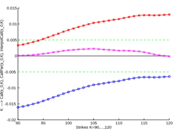
90 95 100 105 110 115 120 -0.02 -0.015 -0.01 -0.005 0 0.005 0.01 0.015 Strikes K=90,...,120
K ---> Call(s_0,K), CallPar(s_0,K), InterpolCall(s_0,K)
Figure 1: Black-Scholes Calls: Error= Reference BS−(MC Premium). K = 90, . . . , 120.
–o–o–o– Crude Call. –∗–∗–∗– Synthetic Parity Call. –×–×–×– Interpolated synthetic Call.
2.3.3 Complexity:
In practical implementation, one often neglects the cost of the computation of λmin since one only
needs a rough estimate or it: this leads to stop its computation after the first 10% or 20% of the simulation.
– In the examples derived form “Parity equations” developed in the above subsection, the r.v. Y is involved in the simulation of X, so the complexity of the simulation process is not increased: updating λM and (the empirical mean) X
′′
M is (almost) costless. Subsequently, in that setting, the
complexity remains the same!
– Warning ! This no longer true in general . . . When the complexity is doubled, the method is efficient iff
σmin2 < 1
2min(Var(X), Var(X′)). if one neglects the cost of the estimation of the coefficient λmin.
2.3.4 Some Simulations ✄Vanilla B-S Calls
Model parameters:
T = 1, x0 = 100, r = 5 %, σ = 20 %, K = 90, . . . , 120.
90 95 100 105 110 115 120 0.1 0.2 0.3 0.4 0.5 0.6 0.7 Strikes K=90,...,120 K ---> lambda(K)
Figure 2: Black-Scholes Calls: K 7→ 1 − λmin(K), K = 90, . . . , 120, for the Interpolated
synthetic Call. 90 95 100 105 110 115 120 4 6 8 10 12 14 16 18 Strikes K=90,...,120
K ---> StD_Call(s_0,K), StD_CallPar(s_0,K), StD_InterpolCall(s_0,K)
Figure 3: Black-Scholes Calls. Standard Deviation(MC Premium). K = 90, . . . , 120.
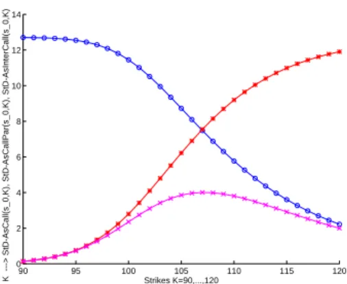
90 95 100 105 110 115 120 0 2 4 6 8 10 12 14 Strikes K=90,...,120
K ---> StD-AsCall(s_0,K), StD-AsCallPar(s_0,K), StD-AsInterCall(s_0,K)
Figure 4: Heston Asian Calls. Standard Deviation (MC Premium). K = 90, . . . , 120.
–o–o–o– Crude Call. –∗–∗–∗– Synthetic Parity Call. –×–×–×– Interpolated synthetic Call.
✄Asian Heston Calls
– The dynamics: Let ϑ, k, a s.t. ϑ2/(2ak) < 1.
dXt = Xt(r dt +√vt)dWt1, X0= x0> 0, (risky asset)
dvt = k(a− vt)dt + ϑ√vtdWt2, v0 > 0 with < W1, W2>t= ρ t, ρ∈ [−1, 1].
– The payoff and the premium: no closed form available for Asian payoffs! AsCallHest= e−rTE ÃÃ 1 T Z T 0 Xsds− K ! + ! .
Note however that (quasi-)closed forms do exist for vanilla European options in this model (see [27]) which is the origin of its success.
– Parameters of the model:
x0 = 100, k = 2, a = 0.01, ρ = 0.5, v0= 10%, ϑ = 20%.
– Parameters of the option portfolio:
T = 1, K = 90,· · · , 120 (31 strikes).
Exercise. One considers a 1-dimensional Black-Scholes model with market parameters r = 0, σ = 0.3, x0 = 100, T = 1
1. One considers a vanilla Call with strike K = 80. The r.v. Y is defined as above. Estimate the λmin (one should be not far from 0.825). Then compute a confidence interval for the Monte
Carlo pricing of the Call with and without the linear variance reduction for the following sizes of the simulation: M = 5 000, 10 000, 100 000, 500 000.
2. Proceed as above but with K = 150 (true price 1.49). What do you observe ? Provide an interpretation.
90 95 100 105 110 115 120 0 0.1 0.2 0.3 0.4 0.5 0.6 0.7 0.8 0.9 1 Strikes K=90,...,120 K ---> lambda(K)
Figure 5: Heston Asian Calls. K 7→ 1 − λmin(K), K = 90, . . . , 120, for the Interpolated
Synthetic Asian Call.
90 95 100 105 110 115 120 −0.02 −0.015 −0.01 −0.005 0 0.005 0.01 0.015 0.02 Strikes K=90,...,120 K −−−> AsCall(s 0 ,K), AsCallPar(s 0 ,K), InterAsCall(s 0 ,K)
Figure 6: Heston Asian Calls. M = 106 (Reference: M C with M = 108). K = 90, . . . , 120.
2.4 Multidimensional case
✄Let X := (X1, . . . , Xd), Y := (Y1, . . . , Yq) : (Ω,A,P)−→Rq, square integrable random vectors.
EX = m∈Rd, E(Y ) = 0∈Rq
Let D(X) := [Cov(Xi, Xj)]
1≤i,j≤d and D(Y ) denote the covariance (dispersion) matrices of X and
Y respectively.
D(X) and D(Y ) > 0 i.e. positive definite symmetric.
✄Problem Find a matrix Λ∈ M(d, q) solution of the optimization problem Var(X− Λ Y ) = min {Var(X − L Y ), L∈ M(d, q)} . ✄Solution
Λ = (D(Y ))−1(C(X, Y )) where
C(X, Y ) = [Cov(Xi, Yj)]1≤i≤d,1≤j≤q. ✄Examples: Traded assets Xt= (X1
t, . . . , Xtd), t∈ [0, T ].
– Options on various baskets Xi = d X j=1 θijXTj − K + , i = 1, . . . , d
Remark. Also produces an optimal asset selection (PCA) which helps for hedging. – Portfolio of forward start options
Xi,j =³XTji+1− XTji
´
+, i = 1, . . . , d
2.5 Importance sampling (introduction to)
The basic principle of importance sampling is the following: let X : (Ω,A,P) → (E, E) be an
E-valued r.v. . Let µ be a σ-finite measure on (E,E) satisfyingP
X ≪ µ i.e. there exists a probability
density f : (E,E) → (R+,B(R+)) such that P
X = f.µ
In practice this means that one has to simulate several r.v. , whose distributions are all absolutely continuous with respect to this reference measure µ. For a first reading one may assume that E =R
and µ is the Lebesgue measure but what follows can also be applied on more general measured spaces like the Wiener space, etc. Then
Eh(X) = Z Eh(x) P X(dx) = Z Eh(x)f (x)µ(dx).
Now for any probability distribution g defined on (E,E) (with respect o µ), one has
Eh(X) = Z E h(x)f (x)µ(dx) = Z E h(x)f (x) g(x) g(x)µ(dx).
One can always enlarge (if necessary) the original probability space (Ω,A,P) to design a random
variable Y : (Ω,A,P) → (E, E) having g as a probability density with respect to µ. Then, going
back on the probability space yields
Eh(X) =E
µh(Y )f (Y )
g(Y )
. (2.3)
So, in order to computeEh(X) on can also implement a Monte Carlo simulation based on the
simulation of independent copies of the r.v. Y i.e.
Eh(X) =E µh(Y )f (Y ) g(Y ) ¶ = a.s. lim M →∞ 1 M M X ℓ=1 h(Yℓ)f (Yℓ) g(Yℓ) .
✄Necessary conditions . . . to undertake the simulation. To proceed it is necessary to simulate Y and to compute the ratio of density functions f /g at a reasonable cost (note that only the ratio is needed which can make useless the computation of some “structural” constants ).
✄Sufficient conditions . . . to undertake the simulation. Once the above conditions are fulfilled, the question is: is it profitable to proceed like that? So is the case if the complexity of the simulation for a given accuracy (in terms of confidence interval) is lower with the second method. If one assume for simplicity that simulating X and Y on the one hand and computing h(x) and (hf /g)(x) on the other hand is comparable the question amounts to comparing the variances.
Now Var µh(Y )f (Y ) g(Y ) ¶ = E µh(Y )f (Y ) g(Y ) ¶2 − (Eh(X))2 = Z E µh(x)f (x) g(x) ¶2 g(x)µ(dx)− (Eh(X))2 = Z E (h(x)f (x))2 g(x) µ(dx)− ( Z Eh(x)µ(dx)) 2
As a consequence simulating Y will reduce the variance iff
Z E (h(x)f (x))2 g(x) µ(dx) < Z E h2(x)f (x)µ(dx).
Remarks. • In fact, theoretically, one may reduce the variance of the new simulation to . . . 0. Assume Eh(X) 6= 0 and g(x) > 0 µ(dx)-a.s.. As a matter of fact, using Schwarz Inequality one
gets, ( Z E h(x)µ(dx))2 = Z E h(x)f (x) p g(x) q g(x)µ(dx) ≤ Z E (h(x)f (x))2 g(x) q g(x)µ(dx)× Z E g dµ = Z E (h(x)f (x))2 g(x) µ(dx)
since g is a probability density. Now the equality case in Schwarz inequality says that the variance is 0 iff pg(x) and h(x)f (x)√
g(x) are µ(dx)-a.s. proportional i.e. h(x)f (x) = cg(x) µ(dx)-a.s. for some
(deterministic) nonnegative real constant c. Finally this leads to g(x) = f (x) h(x)
Eh(X) µ(dx) a.s.
This condition is clearly impossible to reach, the simplest argument being that if it were, this would mean that Eh(X) is known since it is involved in the formula. . . and would then be of no
use. A contrario this may suggest a direction to design the (distribution) of Y .
• The intuition that must guide the user when calling upon some importance sampling method is to replace a r.v. X by another r.v. which is closer to their common mean. When pricing derivatives, the r.v. is a payoff like (XT− K)+which is very often equal to 0 as soon as x0≪ K i.e. the option
is deep-out-of-the money at the origin of time. So the idea is to change the dynamics of the risky asset so that, endowed with its new distribution, it turns to be more often larger than K.
As concerns vanilla option in simple models, one usually work on the state space E =R+ and
importance sampling amounts to a change of variable in integrals. In a more general framework, one works on the scenarii space i.e. one sets (in some way) E = Ω and use Girsanov theorem. Example (option pricing). (a) In a 1-dimensional Black-Scholes model
XTx = x exp (µt + σWT) = x exp (µT + σ
√
T Z), Z =d N (0; 1). Then, a standard change of variable, shows
Eϕ(Xx T) = Eh(Z) = Z R h(x exp (µT + σ√T z)) exp (−z2/2)√dz 2π = Z R
h(x exp (µT + σ√T (u + θ)) exp (−θ2/2− θu − u2/2)√du 2π = exp (−θ2/2)E(exp (−θZ)h(Z + θ))
= exp (θ2/2)E(exp (−θ(Z + θ))h(Z + θ)) .
This identity is sometimes known as the Cameron-Martin formula. Viewed through the above notations related to “abstract” importance sampling, it corresponds to switch from X to Y with
X ←− Z, Y ←− Z + θ
in (2.3) (with the related probability densities). It is to be noticed that there is need to know a numerical value for π. We leave the computations an exercise.
At this stage the underlying idea is to choose a “good” θ. This choice highly depends on the function h as emphasized above.
• If ϕ(x) = (x − K)+ i.e. h(z) = (x exp (µT + σ
√
T z)− K)+, with x ≪ K
(deep-out-of-the-money), most simulations of h(Z) will produce 0 as a result. So, one idea can be to re-center the simulation of XTx around K i.e. choose θ satisfying
E³x exp (µT + σ√T (Z + θ)´= K
which yields θ := log(K/x)
Exercise. Set r = 0, σ = 0.2, X0 = x = 70, T = 1.One wishes to price a Call with strike price
K = 100 (i.e. deep-out-of-the-money). The true Black-Scholes price is 0.248. – Make a “crude” Monte Carlo simulation and then
– apply the above importance sampling
Several methods have been developed to approximate the optimal θ i.e. solution to the mim-imization problem
min θE³exp (θ2/2) exp (−θ(Z + θ))h(Z + θ)´2.
One is based on large deviations techniques (see [20]) seems to be strongly dependent on the regu-larity of the function h (or say the payoff). Another approach based on stochastic approximation techniques has been recently introduced by Arouna in [1]. Although quite promising, one faces a problem: the resulting procedure does not fit (at all) in the regular theory of recursive stochastic algorithms. Practical implementation then often lead to exploding behaviours. To overcome this problem, some further developments are needed, like those developed in [1] which are essentially based on the so-called projection “`a la Chen”.
(b) When dealing with path-dependent options, one usually relies on the Girsanov theorem to modify in an appropriate way the drift of the risky asset dynamics. Of course all this can be implemented for multi-dimensional models. . .
3
Euler scheme(s) of a Brownian diffusion
One considers a d-dimensional Brownian diffusion process (Xt)t∈[0,T ]solution of the following S.D.E.
(SDE) ≡ dXt= b(t, Xt)dt + σ(t, Xt)dWt, (3.4)
where b : [0, T ]×Rd → Rd, σ : [0, T ]×Rd → M(d × q) are continuous functions and (W
t)t∈[0,T ]
denotes a q-dimensional Brownian motion defined on a probability space (Ω,A,P) (the filtration
satisfying the usual conditions). We assume that b and σ are Lipschitz continuous in x uniformly with respect to t i.e., if| . | denotes any norm onRd and k . k any norm on the matrix space,
∀ t∈ [0, T ], ∀ x, y ∈Rd, |b(t, x) − b(t, y)| + kσ(t, x) − σ(t, y)k ≤ K|x − y|.
The starting random variable X0 is defined on (Ω,A,P), square integrable and independent of W .
LetF := (Ft)t∈[0,T ] the (augmented) filtration generated by X0 and σ(Ws, 0≤ s ≤ t).
Then, one shows that the above SDE has a unique strong solution X with initial value X0 (at
time 0). When X0 = x∈Rd one denotes the solution of (SDE) by Xx.
Remark. By adding the component t to X i.e. be setting Yt := (t, Xt) one may always assume
that the (SDE) is homogenous i.e. that the coefficients b and σ only depend on the space variable. This is often enough for applications although it induces some uselessly stringent assumption on the time variable in many theoretical results. Furthermore, when some ellipticity assumptions are required, this way of considering the equation no longer works since the equation dt = 1dt + 0dWt
3.1 Euler-Maruyama schemes: stepwise constant and continuous schemes.
Except for some very specific equations, it is impossible to process an exact simulation of the process X even at a fixed time T (by exact simulation, we mean writing XT = χ(U ), U ∼ U([0, 1]))
(nevertheless, when d = 1 and σ ≡ 1, see [13]). Consequently, to approximate E(f (X
T)) by a
Monte Carlo method, one needs to approximate X by a process that can be simulated (at least at a fixed number of instants). To this end one first introduces the stepwise constant Brownian Euler scheme ¯X = ( ¯XkT
n )0≤k≤n with step
T
n associated to the SDE.
✄Stepwise constant Euler scheme. It is defined by ¯ Xtn k+1 = ¯Xtnk + b(t n k, ¯Xtn k) T n + σ(t n k, ¯Xtn k) s T n Uk+1, X¯0 = X0, k = 0, . . . , n− 1, (3.5) where tn
k = kTn , k = 0, . . . , n− 1 and (Uk)1≤k≤n denotes a sequence of i.i.d. N (0; 1)-distributed
random vectors given by
Uk:= r n T (Wtnk − Wt n k−1), k = 1, . . . , n.
Moreover, set for convenience
t := tnk if t∈ [tnk, tnk+1).
The stepwise constant (sometimes called “discrete”) Euler scheme is defined by
e
Xt= ¯Xt, t∈ [0, T ].
✄Continuous Euler scheme. At this stage it is natural to extend the definition of the Euler scheme at every real instant t∈ [0, T ] by setting
¯
Xt= ¯Xt+ b(t, ¯Xt)(t− t) + σ(t, Xt)(Wt− Wt).
This continuous Euler scheme satisfies (SDE) with frozen coefficients, namely d ¯Xt= b(t, Xt)dt + σ(t, Xt)dWt, X¯0 = X0 i.e. ¯ Xt= X0+ Z t 0 b(s, Xs)ds + Z t 0 σ(s, Xs)dWs.
Then, it is classical background that under the above assumptions on the coefficients b and σ mentioned above, supt∈[0,T ]|Xt− ¯Xt| goes to zero in every Lp(P), 0 < p < ∞. Let us be more
specific on that topic by providing error rates under slightly more stringent assumptions.
How to use this continuous for practical simulation seems not obvious, at least not as obvious as the stepwise constant Euler scheme. However this turns out to be an important method to improve the rate of convergence of M C simulations e.g. for option pricing. Using this scheme in simulation relies on the so-called diffusion bridge method and will be detailed further on.
3.2 Strong error rate
Theorem 5 Assume b and σ satisfies for some index α∈ (0, 1),
∀ t∈ [0, T ], ∀ x, y ∈Rd, |b(s, x) − b(t, y)| + kσ(s, x) − σ(t, y)k ≤ C(|t − s|α+|x − y|) (3.6)
(a) Then, for every n≥ 1, k sup t∈[0,T ]|Xt− ¯ Xt|kp ≤ Cb,σ,peCb,σ,pT(1 +kX0kp) µT n ¶1 2∧α .
In particular if b and σ are Lipschitz in (t, x) the Lp-rate is O(n−12).
(b) Then, for every n≥ 1, k sup t∈[0,T ]|Xt− e Xt|kp≤ Cb,σ,peCb,σ,pT(1 +kX0kp) s log n n .
Remarks. • Note that the second rate is universal since it holds as a sharp rate for the Brownian motion itself k sup t∈[0,T ]|Wt− Wt|kp = k max k=0,...,n−1t∈[tsupn k,tnk+1) |Wt− Wtn k|kp = s T
nkk=0,...,n−1max t∈[k,k+1)sup |Wt− Wk|kp by scaling
≈ s T nCp p log n.
• It follows from the above theorem that the continuous Euler scheme (and the stepwise constant one as well) converge P-a.s. to X. This straightforwardly follows from the Borel-Cantelli Lemma
since for large enough p
X n≥1 E sup t∈[0,T ]|Xt− ¯ Xt|p)≤ c X n≥1 n−p(12∧α)< +∞
which implies that X
n≥1
E sup
t∈[0,T ]|Xt− ¯
Xt|p) < +∞ P-a.s.
One derives likewise some a.s. convergence n−(12∧α−η)-rate or any η small enough.
Beyond these rates, it is often useful to have at hand the following bounds for solutions of (SDE) and its Euler schemes.
Proposition 6 If
∀ t∈ [0, T ], ∀ x∈Rd, |b(t, x)| + kσ(t, x)k ≤ C(1 + |x|)
then, for every p∈ (0, +∞), there exists a real constant Cp,b,σ∈ (0, ∞) such that, for every n ≥ 1,
E sup
t∈[0,T ]|Xt|
p+E sup
t∈[0,T ]| ¯
Xt|p ≤ Cp,b,σ(1 +E|X0|p)eCp,b,σT.
We provide below a partial proof of these results, in the 1-dimensional homogenous case, for the continuous Euler scheme with p = 2 without optimization of the behaviour of the constants (a complete proof can be found e.g. in [14]).
Lemma 2 (Gronwall Lemma) Let f : R+ → R+, a Borel non-negative locally bounded function
and ψ :R+→R+ a non-decreasing function satisfying
(G)≡ f(t) ≤ α
Z t 0
f (s) ds + ψ(t) for some α > 0. Then
∀ t ≥ 0, sup
0≤s≤tf (s)≤ e
αtψ(t).
Proof. It is clear that the non-decreasing (finite) function ϕ(t) := sup0≤s≤tf (s) satisfies (G) instead of f . Now the function e−αtRt
0ϕ(s) ds has right derivative at every t≥ 0 and that
µ e−αt Z t 0 ϕ(s)ds ¶′ r = e−αt(ϕ(t+)− α Z t 0 ϕ(s) ds) ≤ e−αtψ(t+)
Then, it follows from the fundamental theorem of calculus that e−αt Z t 0 ϕ(s)ds− Z t 0 e −αsψ(s+) is non-increasing
so that, applying that between 0 and t yields
Z t
0 ϕ(s)≤ e
αtZ t
0 e
−αsψ(s+)ds
Plugging this in the above inequality implies ϕ(t) ≤ αeαt Z t 0 e −αsψ(s+)ds + ψ(t) = αeαt Z t 0 e−αsψ(s)ds + ψ(t) ≤ eαtψ(t)
where we used successively that a monotone function is ds-a.s. continuous and that ψ is
non-decreasing. ♦
Now we are in position to prove the theorem. For the sake of simplicity, we will assume that d = 1, p = 2 and that the diffusion is homogenous with Lipschitz coefficients. Furthermore, we will not try dealing with the constants in an optimal way.
Doob’s Inequality. (see e.g. [33]) Let M = (Mt)t≥0 be a continuous time martingale. Then, for
every T > 0, E Ã sup t∈[0,T ] Mt2 ! ≤ 4EM2 T = 4E < M >T .
Proof of Theorem 5 (partial). Step 1. Let τL :=∈ {t : |Xt− X0| ≥ L}, L ∈ N\ {0}. It is a
positive F-stopping times and |XτL
t | ≤ L + |X0| for every t∈ [0, ∞). Then, using the local feature
of standard and stochastic integral leads to XτL t = X0+ Z t∧τL 0 b(XτL s )ds + Z τL 0 σ(XτL s )dWs.
The continuous local martingale Mt(n):=Rt∧τL
0 σ(X
τL
s )XτLdWsis a true square integrable
martin-gale since < M(L)>t= Z t∧τL 0 σ 2(XτL s )ds≤ C(1 + L2+ X02)t∈ L1(P)
where we used that|σ(x)| ≤ Cσ(1 +|x|). Consequently, using that b also has at most linear growth,
that t∧ τL≤ t, one derives that
sup s∈[0,t] (XτL s )2 ≤ 3 Ã X02+ µZ t∧τn 0 Cb(1 +|X τL s |)ds ¶2 + sup s∈[0,t]|M (L) s |2 ! .
Consequently, using Schwarz inequality to make the square “shift down” inside the “time” integral and Doob Inequality for the stochastic integral yield
E( sup s∈[0,t] (XτL s )2)≤ Cb,σ,T Ã EX2 0 + Z t 0 (1 +E( sup u∈[0,s] (XτL u )2))ds +E Z τL∧t 0 (Cσ(1 +|XsτL|))2ds ! . This can be rewritten (using that τL∧ t ≤ t),
E( sup s∈[0,t] (XτL s )2)≤ Cb,σ,T Ã 1 +EX2 0 + Z t 0 E( sup u∈[0,s] (XτL u )2)ds ! . Gronwall Lemma implies that
E( sup
s∈[0,t]
(XτL
s )2)≤ Cb,σ,T(1 +EX02)eCb,σ,Tt.
This holds or every L≥ 1 so that Fatou’s lemma implies
E( sup
s∈[0,T ]
Xs2)≤ Cb,σ,T(1 +EX02)eCb,σ,TT = Cb,σ,T′ (1 +EX02).
The same approach works for the Euler scheme (introduce¯τLfor ¯X and note that supu∈[0,s]| ¯Xu| ≤
supu∈[0,s]| ¯Xu|. This yields
sup
n≥1
E( sup
s∈[0,T ]
( ¯Xs)2)≤ Cb,σ,T(1 +EX02)eCb,σ,TT.
Step 2: Combining the equations satisfied by X and its (continuous )Euler scheme yields Xt− ¯Xt = Z t 0 (b(Xs)− b( ¯Xs))ds + Z t 0 (σ(Xs)− σ( ¯Xs))dWs
Consequently, using that b and σare Lipschitz and Doob Inequality lead to
E sup s∈[0,t]|Xs− ¯ Xs|2 ≤ 2E µZ t 0 [b]Lip|Xs− ¯Xs|ds ¶2 + 2E sup s∈[0,t] µZ s 0 ((σ(Xu)− σ( ¯Xu))dWu ¶2 ≤ 2E µZ t 0 [b]Lip|Xs− ¯Xs|ds ¶2 + 8E Z t 0 ((σ(Xu)− σ( ¯Xu))2du ≤ 2E µZ t 0 [b]Lip|Xs− ¯Xs|ds ¶2 + 8[σ]2Lip Z t 0 E|Xu− ¯Xu|2du ≤ Cb,σ,T Z t 0 |Xs− ¯Xs| 2ds ≤ Cb,σ,T Z t 0 E sup u∈[0,s]|Xu− ¯ Xu|2ds + Cb,σ,T Z t 0 E| ¯Xs− ¯Xs|2ds.