Machine Learning for Financial Products Recommendation

HAL Id: tel-02974918

https://tel.archives-ouvertes.fr/tel-02974918

HAL is a multi-disciplinary open access archive for the deposit and dissemination of sci-entific research documents, whether they are pub-lished or not. The documents may come from teaching and research institutions in France or abroad, or from public or private research centers.

L’archive ouverte pluridisciplinaire HAL, est destinée au dépôt et à la diffusion de documents scientifiques de niveau recherche, publiés ou non, émanant des établissements d’enseignement et de recherche français ou étrangers, des laboratoires publics ou privés.

Machine Learning for Financial Products

Recommendation

Baptiste Barreau

To cite this version:

Baptiste Barreau. Machine Learning for Financial Products Recommendation. Computational Engi-neering, Finance, and Science [cs.CE]. Université Paris-Saclay, 2020. English. �NNT : 2020UPAST010�. �tel-02974918�

Machine Learning for Financial

Products Recommendation

Apprentissage Statistique pour la Recommandation

de Produits Financiers

Thèse de doctorat de l'université Paris-Saclay

École doctorale n°573

Interfaces : Approches interdisciplinaires, fondements, applications et

innovation

Thèse présentée et soutenue à Gif-sur-Yvette, le 15

septembre 2020, par

Baptiste BARREAU

Composition du Jury

Professeur, École Polytechnique Président

Charles-Albert LEHALLE

Head of Data analytics, Capital Fund Management, HDR Rapporteur & Examinateur Elsa NEGRE

Maître de conférences, Université Paris-Dauphine, HDR Rapporteur & Examinatrice Eduardo ABI JABER

Maître de conférences, Université Paris 1 Examinateur

Sylvain ARLOT

Professeur, Université Paris-Sud Examinateur

Damien CHALLET

Professeur, CentraleSupélec Directeur de thèse

Sarah LEMLER

Maître de conférences, CentraleSupélec Co-Directrice de thèse

Frédéric ABERGEL

Professeur, BNP Paribas Asset Management Invité

Laurent CARLIER

Head of Data & AI Lab, BNPP CIB Global Markets Invité

Th

ès

e

de

d

oc

to

ra

t

:

20

20

U

PAS

T0

10

Résumé

L’anticipation des besoins des clients est cruciale pour toute entreprise — c’est particulièrement vrai des banques d’investissement telles que BNP Paribas Corporate and Institutional Banking au vu de leur rôle dans les marchés financiers. Cette thèse s’intéresse au problème de la pré-diction des intérêts futurs des clients sur les marchés financiers, et met plus particulièrement l’accent sur le développement d’algorithmes ad hoc conçus pour résoudre des problématiques spécifiques au monde financier.

Ce manuscrit se compose de cinq chapitres, répartis comme suit:

- Le chapitre 1 expose le problème de la prédiction des intérêts futurs des clients sur les marchés financiers. Le but de ce chapitre est de fournir aux lecteurs toutes les clés néces-saires à la bonne compréhension du reste de cette thèse. Ces clés sont divisées en trois parties: une mise en lumière des jeux de données à notre disposition pour la résolution du problème de prédiction des intérêts futurs et de leurs caractéristiques, une vue d’ensemble, non exhaustive, des algorithmes pouvant être utilisés pour la résolution de ce problème, et la mise au point de métriques permettant d’évaluer la performance de ces algorithmes sur nos jeux de données. Ce chapitre se clôt sur les défis que l’on peut rencontrer lors de la conception d’algorithmes permettant de résoudre le problème de la prédiction des intérêts futurs en finance, défis qui seront, en partie, résolus dans les chapitres suivants; - Le chapitre 2 compare une partie des algorithmes introduits dans le chapitre 1 sur un jeu

de données provenant de BNP Paribas CIB, et met en avant les difficultés rencontrées pour la comparaison d’algorithmes de nature différente sur un même jeu de données, ainsi que quelques pistes permettant de surmonter ces difficultés. Ce comparatif met en pratique des algorithmes de recommandation classiques uniquement envisagés d’un point de vue théorique au chapitre précédent, et permet d’acquérir une compréhension plus fine des différentes métriques introduites au chapitre 1 au travers de l’analyse des résultats de ces algorithmes;

- Le chapitre 3 introduit un nouvel algorithme, Experts Network, i.e., réseau d’experts, conçu pour résoudre le problème de l’hétérogénéité de comportement des investisseurs d’un marché donné au travers d’une architecture de réseau de neurones originale, inspirée de la recherche sur les mélanges d’experts. Dans ce chapitre, cette nouvelle méthodologie est utilisée sur trois jeux de données distincts: un jeu de données synthétique, un jeu de données en libre accès, et un jeu de données provenant de BNP Paribas CIB. Ce chapitre présente aussi en plus grand détail la genèse de l’algorithme et fournit des pistes pour l’améliorer;

- Le chapitre 4 introduit lui aussi un nouvel algorithme, appelé History-augmented

collabora-tive filtering, i.e., filtrage collaboratif augmenté par historiques, qui proposes d’augmenter

des clients et produits considérés. Ce chapitre poursuit l’étude du jeu de données étudié au chapitre 2 et étend l’algorithme introduit avec de nombreuses idées. Plus précisément, ce chapitre adapte l’algorithme de façon à permettre de résoudre le problème du cold

start, i.e., l’incapacité d’un système de recommandation à fournir des prédictions pour de

nouveaux utilisateurs, ainsi qu’un nouveau cas d’application sur lequel cette adaptation est essayée;

- Le chapitre 5 met en lumière une collection d’idées et d’algorithmes, fructueux ou non, qui ont été essayés au cours de cette thèse. Ce chapitre se clôt sur un nouvel algorithme mariant les idées des algorithmes introduits aux chapitres 3 et 4.

La recherche présentée dans cette thèse a été conduite via le programme de thèses CIFRE, en col-laboration entre le laboratoire MICS de CentraleSupélec et la division Global Markets de BNP Paribas CIB. Elle a été conduite dans le cadre du mandat de l’équipe Data & AI Lab, une équipe de science des données faisant partie de la recherche quantitative et dévouée à l’application des méthodes d’apprentissage statistique aux problématiques des différentes équipes de Global Mar-kets.

Mots-clés. Apprentissage statistique, finance, systèmes de recommandation, clustering su-pervisé, systèmes de recommandation dépendants du contexte, systèmes de recommandation dépendants du temps, apprentissage profond, réseaux de neurones.

Abstract

Anticipating clients’ needs is crucial to any business — this is particularly true for corporate and institutional banks such as BNP Paribas Corporate and Institutional Banking due to their role in the financial markets. This thesis addresses the problem of future interests prediction in the financial context and focuses on the development of ad hoc algorithms designed for solving specific financial challenges.

This manuscript is composed of five chapters:

- Chapter 1 introduces the problem of future interests prediction in the financial world. The goal of this chapter is to provide the reader with all the keys necessary to understand the remainder of this thesis. These keys are divided into three parts: a presentation of the datasets we have at our disposal to solve the future interests prediction problem and their characteristics, an overview of the candidate algorithms to solve this problem, and the development of metrics to monitor the performance of these algorithms on our datasets. This chapter finishes with some of the challenges that we face when designing algorithms to solve the future interests problem in finance, challenges that will be partly addressed in the following chapters;

- Chapter 2 proposes a benchmark of some of the algorithms introduced in Chapter 1 on a real-word dataset from BNP Paribas CIB, along with a development on the difficulties encountered for comparing different algorithmic approaches on a same dataset and on ways to tackle them. This benchmark puts in practice classic recommendation algorithms that were considered on a theoretical point of view in the preceding chapter, and provides further intuition on the analysis of the metrics introduced in Chapter 1;

- Chapter 3 introduces a new algorithm, called Experts Network, that is designed to solve the problem of behavioral heterogeneity of investors on a given financial market using a custom-built neural network architecture inspired from mixture-of-experts research. In this chapter, the introduced methodology is experimented on three datasets: a synthetic dataset, an open-source one and a real-world dataset from BNP Paribas CIB. The chapter provides further insights into the development of the methodology and ways to extend it; - Chapter 4 also introduces a new algorithm, called History-augmented Collaborative

Filter-ing, that proposes to augment classic matrix factorization approaches with the information

of users and items’ interaction histories. This chapter provides further experiments on the dataset used in Chapter 2, and extends the presented methodology with various ideas. Notably, this chapter exposes an adaptation of the methodology to solve the cold-start problem and applies it to a new dataset;

- Chapter 5 brings to light a collection of ideas and algorithms, successful or not, that were experimented during the development of this thesis. This chapter finishes on a new

algorithm that blends the methodologies introduced in Chapters 3 and 4.

The research presented in this thesis has been conducted under the French CIFRE Ph.D. pro-gram, in collaboration between the MICS Laboratory at CentraleSupélec and the Global Mar-kets division of BNP Paribas CIB. It has been conducted as part of the Data & AI Lab mandate, a data science team within Quantitative Research devoted to the applications of machine learn-ing for the support of Global Markets’ business lines.

Keywords. Machine learning, finance, recommender systems, supervised clustering, context-aware recommender systems, time-context-aware recommender systems, deep learning, neural net-works.

Contents

Résumé i

Abstract iii

Acknowledgements 5

1 Recommendations in the financial world 7

1.1 Predicting future interests . . . 7

1.1.1 Enhancing sales with recommender systems . . . 7

1.1.2 An overview of bonds and options . . . 9

1.2 Understanding data . . . 12

1.2.1 Data sources . . . 12

1.2.2 Exploring the heterogeneity of clients and assets . . . 13

1.3 A non-exhaustive overview of recommender systems . . . 14

1.3.1 Benchmarking algorithms . . . 16

1.3.2 Content-filtering strategies . . . 17

1.3.3 Collaborative filtering strategies . . . 19

1.3.4 Other approaches . . . 26

1.3.5 The cold-start problem . . . 27

1.4 Evaluating financial recommender systems . . . 27

1.4.1 Deriving symmetrized mean average precision . . . 27

1.4.2 A closer look at area under curve metrics . . . 30

1.4.3 Monitoring diversity . . . 31

1.5 The challenges of the financial world . . . 32

2 First results on real-world RFQ data 35 2.1 From binary to oriented interests . . . 35

2.2 A benchmark of classic algorithms . . . 36

2.2.1 Historical models . . . 36

2.2.2 Resource redistribution models . . . 37

2.2.3 Matrix factorization models . . . 39

2.2.4 Gradient tree-boosting models . . . 40

2.2.5 Overall benchmark . . . 41

2.3 Concluding remarks . . . 42

3 A supervised clustering approach to future interests prediction 43 3.1 Heterogeneous clusters of investors . . . 44

3.1.1 Translating heterogeneity . . . 44

3.1.2 Non-universality of investors . . . 45

3.2 Introducing Experts Network . . . 47

3.2.1 Architecture of the network . . . 47

3.2.2 Disambiguation of investors’ experts mapping . . . 48

3.2.3 Helping experts specialize . . . 49

3.2.4 From gating to classification . . . 49

3.2.5 Limitations of the approach . . . 50

3.3 Experiments . . . 50

3.3.1 Synthetic data . . . 50

3.3.2 IBEX data . . . 55

3.3.3 BNPP CIB data . . . 58

3.4 A collection of unfortunate ideas . . . 59

3.4.1 About architecture . . . 59

3.4.2 About regularization . . . 61

3.4.3 About training . . . 62

3.5 Further topics in Experts Networks . . . 63

3.5.1 Boosting ExNets . . . 63

3.5.2 Towards a new gating strategy . . . 64

3.6 Concluding remarks . . . 65

4 Towards time-dependent recommendations 67 4.1 Tackling financial challenges . . . 67

4.1.1 Context and objectives . . . 67

4.1.2 Related work . . . 68

4.2 Enhancing recommendations with histories . . . 69

4.2.1 Some definitions . . . 69

4.2.2 Architecture of the network . . . 70

4.2.3 Optimizing HCF . . . 70

4.2.4 Going further . . . 71

4.3 Experiments . . . 71

4.3.1 Evolution of forward performance with training window size . . . 72

4.3.2 Evolution of forward performance with time . . . 74

4.3.3 Evolution of forward performance with history size . . . 75

4.4 Further topics in history-augmented collaborative filtering . . . 75

4.4.1 Sampling strategies . . . 76

4.4.2 Evolution of scores with time . . . 77

4.4.3 Solving cold-start . . . 78

4.4.4 Application to primary markets of structured products . . . 81

4.5 Concluding remarks . . . 83

5 Further topics in financial recommender systems 85 5.1 Mapping investors’ behaviors with statistically validated networks . . . 85

5.2 A collection of small enhancements . . . 89

5.2.1 A focal version of Bayesian Personalized Ranking . . . 89

5.2.2 Validation strategies in non-stationary settings . . . 90

5.2.3 Ensembling with an entropic stacking strategy . . . 91

5.3 First steps towards lead-lag detection . . . 93

5.3.1 Simulating lead-lag . . . 94

5.3.2 A trial architecture using attention . . . 95

5.3.3 First experimental results . . . 96

Conclusions and perspectives 101 Conclusions et perspectives 103 Bibliography 105 List of Figures 115 List of Tables 117 Glossary 119

A Basics of deep learning 121

A.1 General principles of neural networks . . . 121

A.1.1 Perceptrons . . . 121

A.1.2 Multi-layer perceptrons . . . 123

A.1.3 Designing deep neural networks . . . 124

A.2 Stochastic gradient descent . . . 125

A.2.1 Defining the optimization problem . . . 125

A.2.2 Deriving the SGD algorithm . . . 126

A.2.3 A couple variations of SGD . . . 127

A.3 Backpropagation algorithm . . . 128

Acknowledgements

I would like to express my gratitude to Frédéric Abergel and Laurent Carlier for providing me with the opportunity to conduct this Ph.D. thesis within BNP Paribas Corporate and Institutional Banking. Thanks to Frédéric Abergel for accepting to be my academic Ph.D. supervisor, and for his initial and precious guidance on my research. Many thanks to Damien Challet, who took over the supervision of my thesis for the last two years and who, thanks to his academic support and his deep and thoughtful questions, fueled me with the inspiration I required to pursue this work. Thanks also to Sarah Lemler for following my work, even remotely, and for her help when I needed it.

I would also like to thank the fantastic Global Markets Data & AI Lab team as a whole and, more particularly, its Parisian division for their welcome and all the good times we spent together during these past three years. Many thanks to Laurent Carlier for being my industrial Ph.D. supervisor and our countless and fruitful discussions on our research ideas. Thanks to Julien Dinh for following my work and examining it with his knowledgeable scrutiny. Special thanks to William Benhaim, François-Hubert Dupuy, Amine Amiroune, the more recent Jeremi Assael and Alexandre Philbert, and our two graduate program rotations, Victor Geoffroy and Jean-Charles Nigretto, for our fruitful discussions and our pub crawls that, without doubt, fueled the creativity required for this work. Many thanks also to the interns Lola Moisset, Dan Sfedj, Camille Garcin, and Yassine Lahna, with whom I had the chance to work on topics related to the research presented in this manuscript and deepen my knowledge of the presented subjects. I am sincerely grateful to my family as a whole and more particularly to my parents, Annick and Bruno Barreau, for their love and support during my entire academic journey, which ends with this work. My deepest thanks go to the one who shares my life, Camille Raffin, for her unconditional support and her heartwarming love, in both good and bad times.

Chapter 1

Recommendations in the financial

world

Mathematics have made their appearance in corporate and institutional banks in the 90s with the development of quantitative research teams. Quantitative researchers, a.k.a. quants, are devoted to applying all tools of mathematics to help the traders and salespeople, a.k.a. sales, of the bank. Quants have historically focused on developing tools and innovations for the use of traders — the recent advances of machine learning, however, have allowed them to provide new kinds of solutions for the previously overlooked salespeople. Notably, deep learning methodolo-gies allow assisting sales with their daily tasks in many ways, from automating repetitive tasks by leveraging natural language processing tools to providing decision-support algorithms such as recommender systems. This thesis provides an in-depth exploration of recommender systems, their application to the context of a corporate and investment bank, and how we can improve models from literature to better suit the characteristics of the financial world.

This chapter introduces the context and research question examined in this thesis (Section 1.1), elaborates on and explores the data we use (Section 1.2), gives an overview of recommender systems (Section 1.3), sets the evaluation strategy that we use in all further experiments (Section 1.4) and provides insights into the challenges we face in a financial context (Section 1.5).

1.1 Predicting future interests

This section introduces the financial context, defines the recommendation problem that we want to solve, and provides first insights into the datasets we study.

1.1.1 Enhancing sales with recommender systems

BNP Paribas CIB is a market maker. The second Markets in Financial Instruments Directive, MiFID II, a directive of the European Commission for the regulation of financial markets, defines a market maker as "a person who holds himself out on the financial markets on a continuous basis as being willing to deal on own account by buying and selling financial instruments against that person’s proprietary capital at prices defined by that person," see (The European Commission, 2014, Article 4-7).

Market makers play the role of liquidity providers in the financial markets by quoting both buy and sell prices for many different financial assets. From the perspective of a market maker, a.k.a. the sell side, we call bid the buy price and ask the sell price, with pbid < pask. Consequently, on

maker is driven by the bid-ask spread, i.e., the difference between bid and ask prices — the role of a market maker is therefore not to invest in the financial markets but to offer investors the opportunity to do so. The perfect situation happens when the market maker directly finds buyers and sellers for the same financial product at the same time. However, this ideal case is not common, and the bank has to suffer risk from holding products before they are bought by an investor or from stocking products to cope with demand. These assets, called axes, need to be carefully managed to minimize the risk to which the bank is exposed. This management is part of the role of traders and sales, and has notably been studied in Guéant et al. (2013). Sales teams are the interface between the bank and its clients. When a client wants to buy or sell a financial asset, she may call a sales from a given bank, or directly interact with market makers on an electronic platform such as the Bloomberg Dealer-to-Client (D2C) one (Bloomberg, 2020). It can happen that a client does not want to buy/sell a given product at the moment of the sales’ call, but shows interest in it. Sales can then register an indication of interest (IOI) in BNPP CIB systems, a piece of valuable information for further commercial discussions, and for the prediction of future interests. On D2C platforms, clients can request prices from market makers in two distinct processes called request for quotation (RFQ) and request for market (RFM). RFQs are directed, meaning that these requests are specifically made for either a buy or sell direction, whereas RFMs are not. RFMs can be seen as more advantageous to the client, as she provides less information about her intent in this process. However, for less liquid assets such as bonds, the common practice is to perform RFQs. Market makers continuously stream bid and ask prices for many assets on D2C platforms. When a client is interested in a given product, she can select n providers and send them an RFQ — providers then respond with their final price, and the client chooses to buy or sell the requested product with either one of these n providers, or do nothing. Only market makers among these n receive information about the client’s final decision. A typical value of n is 6, such as for the Bloomberg D2C platform. Fermanian et al. (2016) provide an extensive study along with a modeling of the RFQ process. Responding to calls and requests is the core of a sales’ work. But sales can also directly contact clients and suggest relevant trade ideas to them, e.g., assets on which the bank is axed and for which it might offer a better price than its competitors. This proactive behavior is particularly important for the bank as it helps manage financial inventories and better serve the bank’s clients when their needs are correctly anticipated.

Correctly anticipating clients’ needs and interests, materialized by the requests they perform, is therefore of particular interest to the bank. Recommender systems, defined as "an information-filtering technique used to present the items of information (video, music, books, images, Web-sites, etc.) that may be of interest to the user" (Negre, 2015), could help us better anticipate these requests and support the proactive behavior of sales by allowing them to navigate the complexity of markets more easily. Consequently, the research problem that we try to solve in this thesis is the following:

At a given date, which investor is interested in buying and/or selling a given financial asset?

This thesis aims at designing algorithms that try to solve this open question while being well-suited to the specificities of the financial world, further examined in Section 1.5.

1.1.2 An overview of bonds and options

The mandate of the Data & AI Lab covers multiple asset classes, from bonds to options on equity or foreign exchange market, as known as FX. In-depth knowledge of these financial products is not required to understand the algorithms that are developed in this thesis. However, it is essential to know what these products and their characteristics are to design relevant methodologies. This section consequently provides an overview of the financial assets that will be covered in this thesis. It does not require prior knowledge of mathematical finance, and only aims at providing insights into the main characteristics and properties of these assets. An in-depth study of financial assets can be found in Hull (2014).

Bonds

It is possible to leverage financial markets to issue debt in the form of bonds. Fabozzi (2012, Chapter 1) defines a bond as "a debt instrument requiring the issuer to repay to the lender the amount borrowed plus interest over a specified period of time." There are three main types of bonds, defined by their issuer — municipal bonds, government bonds, and corporate bonds. The definitions and examples provided in this section are freely inspired by Hull (2014, Chap-ter 4).

Bonds, as other financial assets, are issued on primary markets, where investors can buy them for a limited period of time. In the context of equities, initial public offerings (IPO) are an example of a primary market. The issuance date of a bond corresponds to its entry on the

secondary market. On the secondary market, investors can freely trade bonds before their maturity date, .i.e., their expiry date. Consequently, bonds have a market price determined by

bid and ask, and usual features related to its evolution can be computed.

Figure 1.1: Cash flows of a bond.

The interest rate of a bond is usually defined annually. Interests are either paid periodically as

coupons or in full at maturity, in which case the bond is called a zero-coupon. The cash flows

of a bond are summed up in Fig. 1.1. Classically, coupons are paid on a semiannual basis. Bonds are expressed in percent, i.e., the value of a bond at issuance is considered to be 100. For example, the value of a semiannual coupon bond with an interest rate of 10% a year after issuance is 100 ú 1.05 ú 1.05 = 110.25. If we consider a compounding of m times per annum, the terminal value of an investment of 100 at rate R after n years is given by 100 ú (1 + R/m)mn_.

Considering the m æ Œ limit, it can be shown that the terminal value converges to 100 ú eRn_.

This is known as continuous compounding and is used for further computations.

The theoretical price of a bond is defined as the present value of the future cash flows received by the owner of the bond. Future cash flows are discounted using the Treasury zero-coupon rates maturing at the time of these cash flows, as Treasury bonds are considered risk-free. For instance, in the case of a 2-year bond with a 6% rate delivering semiannual coupons, the

theoretical price of the bond pt, expressed in basis points, is defined as pt = 3e≠T0.5ú0.5 +

3e≠T1.ú1._+3e≠T1.5ú1.5_+103e≠T2.ú2._{, where Tn is the n-year Treasury zero-coupon rate. The yield} y of a bond is defined as the single discount rate that equals the theoretical bond price, i.e., in

basis points, pt= 3e≠yú0.5+3e≠yú1.+3e≠yú1.5+103e≠yú2.. The yield can be found using iterative

methods such as Newton-Raphson. High yields can come from either high coupons or a low theoretical bond value — its interpretation is consequently subject to caution. It is, however, a useful quantity to understand bonds, and yield curves representing yield as a function of maturity for zero-coupon government bonds are often used to analyze rates markets. The bond

spread corresponds to the difference, expressed in basis points, between the bond yield and the

zero-coupon rate of a risk-free bond of the same maturity.

Another useful quantity is the duration of a bond. Noting ci, i œ [[1; n]] the cash flow at time

ti, the theoretical bond price can be written pt=qni=1cie≠yti, where y denotes the yield. The

duration of the bond is then defined as

Dt= qn i=1ticie≠yti pt = n ÿ i=1 ti C cie≠yti pt D . (1.1)

Duration can be understood as a weighted average of payment times with a weight corresponding to the proportion of the bond’s total present value provided by the i-th cash flow. It consequently measures how long on average an investor has to wait before receiving payments.

Finally, bonds also receive a credit rating representing the credit worthiness of their issuer. Credit rating agencies such as Moody’s or Standard & Poors publish them regularly for both corporate and governmental bonds. As they are meant to indicate the likelihood that the debt will be fully repaid, investors use such ratings to guide their investment choices.

More information about interest rates in general and bonds in particular can be found in Hull (2014, Chapter 4). In this work, we cover corporate and G10 bonds, i.e., governmental bonds from countries of the G10 group (Germany, Belgium, Canada, United States, France, Italy, Japan, Netherlands, United Kingdom, Sweden, Switzerland).

Options

Hull (2014, Chapter 10) defines options as financial contracts giving holders the right to buy or sell an underlying asset by (or at) a certain date for a specific price. The right to buy an underlying asset is named a call option, and the right to sell is named a put option. The price at which the underlying asset can be bought/sold is called the strike price. The date at which the underlying asset can be bought/sold is called the maturity date, as in bonds. If the option allows exercising this right at any time before maturity, it is said to be American. If the right can only be exercised at maturity, the option is said to be European. American options are the most popular ones, but we consider here European options for ease of analysis. Investors have to pay a price to acquire an option, regardless of the exercise of the provided right.

Options can be bought or sold, and can even be traded. Buyers of options are said to have long

positions, and sellers are said to have short positions. Sellers are also said to write the option.

Figure 1.2 shows the four different cases possible and their associated payoffs.

To understand the interest of options, let us take the example of an investor buying a European call option for 100 shares of a given stock with a strike price of 50Ä at a price of 5Ä per share. Assume the price at the moment of the contract was 48Ä. If at maturity, the price of the stock is 57Ä, the investor exercises its right to buy 100 shares of the stock at 50Ä and directly sells them. She makes a net profit of 700-500=200Ä. If the investor would have invested the same amount in the stock directly, she would have made a profit of 9Ä per share and could have

Figure 1.2: The four different options payoff structures. (·)+ denotes here max (·, 0).

bought only 4 of them, making a net profit of 36Ä. Options are leverage instruments: for the same amount of money invested, they provide the opportunity to obtain far better returns at the cost of higher risk. We see in this example that at prices below 55Ä, the options investor would start losing money, whereas the buyer of the shares would still make a profit.

In the case of equity options, Hull (2014, Chapter 11) enumerates six factors affecting the price of an option:

- the current price of the equity, noted S0;

- the strike price K; - the time to maturity T ;

- the volatility of the underlying ‡; - the risk-free interest rate r;

- the dividends D expected to be paid, if any.

Using the no-arbitrage principle stating that there are no risk-free investments insuring strictly positive returns, an analysis of these factors allows deriving lower and upper bounds on the option price (Hull, 2014, Chapter 11). The arbitrage analysis allows as well to uncover the

call-put parity. This property links call and put prices by the formula:

Ccall+ Ke≠rT + D = Cput+ S0, (1.2)

considering that stocks with no dividends have D = 0.

The price of an option can be derived analytically using stochastic calculus. If we assume, among other hypotheses that one can find in Hull (2014, Chapter 15), that stock prices follow a geometric Brownian motion dSt = St(µdt + ‡dBt) where µ is the drift and ‡ the volatility,

we can derive the Black-Scholes equation (Black and Scholes, 1973):

ˆC ˆt + rS ˆC ˆS + 1 2‡2S2 ˆ2C ˆS2 ≠ rC = 0, (1.3)

where C is the price of the (European) option, S the price of the underlying, ‡ the volatility of the underlying and r the risk-free rate. Notably, this equation links the price of the option to the volatility of the underlying. Using the bounds found in the arbitrage analysis, the equation can be used both to derive the price of an option using the historical volatility computed from past prices of its underlying and to determine the implied volatility from the option current price. Implied volatility is an indicator that is used for markets analysis, and can serve as input in more complex models.

Moreover, calls and puts can be combined in option strategies to form new payoff structures. Classic combinations include the following:

- Call spread. A call spread is the combination of a long call at a given strike and a short call at a higher strike. The payoff corresponds to the one of a call, with a cap on the maximum profit possible. Call spreads allow benefiting from a moderate increase in price, at a lower cost than a classic call option.

- Put spread. A put spread is the combination of a short put at a given strike and a long put at a higher strike. The payoff corresponds to the one of a put, with a cap on the maximum profit possible. Put spreads allow benefiting from a moderate decrease in price, at a lower cost than a classic put option.

- Straddle. Buying a straddle corresponds to buying a call and a put with the same strike prices and maturities on the same underlying. This position is used in high volatility situations when an investor reckons that the underlying price might evolve a lot in either direction.

- Strangle. Buying a strangle corresponds to buying a call and a put with the maturities on the same underlying, but with different strike prices. This position is used in the same situation as a straddle, but can be bought at a lower price.

1.2 Understanding data

We introduced the global characteristics of the RFQ datasets that are studied in this thesis in Section 1.1. However, an in-depth exploration of the data is required to understand the chal-lenges that lie within data: from this exploration follow insights that can guide the construction of an algorithm tailored to face these challenges. Consequently, this section explains the data sources at hand and provides an exploratory analysis of a particularly important characteristic of the datasets we study in this thesis.

1.2.1 Data sources

To solve the problem exposed in Section 1.1, we have various sources of data at our disposal. For all the asset classes that we may consider, we count three data categories.

- Client-related data. When an investor becomes a BNPP CIB client, she fills Know

Your Customer (KYC) information that can be used in our models, such as her sector

of activity, her region, . . . , i.e., a set of categorical features. Due to their size and/or the nature of their business, some clients may also have to periodically report the content of their portfolio. This data is particularly valuable, as an investor cannot sell an asset she does not have. Consequently, knowing their portfolio allows for more accurate predictions — in particular, in the sell direction.

- Asset-related data. Financial products are all uniquely identified in the markets by their International Securities Identification Number (ISIN, 2020). Depending on the nature of the asset, categorical features can be derived to describe it. For instance, bonds can be described through their issuer, also known as the ticker of the bond, the sector of

activity of the latter, the currency in which it was issued, its issuance and maturity dates, . . . Market data of the assets can also be extracted, i.e., numerical features such as the price, the volatility or other useful financial indicators. Usually, these features are recorded on a daily basis at their close value, i.e., their value at the end of the trading day. For options, both market data for the option and its underlying can be extracted.

- Trade-related data. The most important data for recommender systems is the trade-related one. This data corresponds to all RFQs, RFMs, and IOIs that were gathered by sales teams (see Section 1.1.1). These requests and indications of interest provide us with the raw interest signal of a client for a given product. As the final decision following a request is not always known, we use the fact that a client made a request on a particular product as a positive event of interest for that product.

These different sources are brought together in various ways depending on the algorithms that we use, as exposed in Section 1.3 and in the next chapters of this thesis.

1.2.2 Exploring the heterogeneity of clients and assets

An essential characteristic of our RFQ datasets, common to many fields of application, is hetero-geneity. Heterogeneity of activity is deeply embedded in our financial datasets and appears on both the client and asset sides. We explore here the case of the corporate bonds RFQ database, studying a portion ranging from 07/01/2017 to 03/01/2020. In this period, we count roughly 4000 clients and 30000 bonds. Of these 4000 clients, about 23% regularly disclose the content of their bond portfolios — this information is consequently difficult to use in a model performing predictions for all clients.

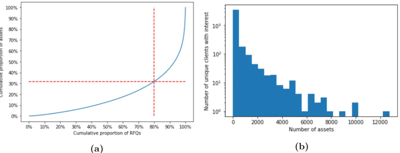
Let us begin with the heterogeneity of clients. A glimpse at heterogeneity can be taken by looking at a single client: the most active client accounted for 5% of all performed RFQs alone, and up to 6.4% when taking into account all its subsidiaries. The heterogeneity of clients can be further explored with Fig. 1.3. In Fig. 1.3a, we see that 80% of the accounted RFQs were made by less than 10% of the client pool. Most of BNPP CIB business is consequently done with a small portion of its client reach: a recommender system could help better serve this portion of BNPP clients by providing sales with offers tailored to their needs. The histogram shown in Fig. 1.3b provides another visualization of this result. We see here that a few clients request prices for thousands of unique bonds, whereas over the same period, some clients only request prices for a handful of bonds. Clients are consequently profoundly heterogeneous. Note however that this heterogeneity, to some extent, might only be perceived as such as we do not observe the complete activity of our clients and only what they do on platforms on which BNPP CIB is active.

We now give a closer look at the heterogeneity of bonds. In particular, here, the most active bond accounted for 0.3% of all RFQs, and up to 1% when aggregating all bonds emitted by the same issuer. A global look at these statistics is presented in Fig. 1.4a. To avoid bias from expiring products, we only account in this graph for bonds with issue and maturity dates strictly outside of the considered period. We see here that 80% of the RFQs were done on more than 30% of the considered assets. The heterogeneity of bonds is consequently less pronounced that the heterogeneity of clients. There are however more pronounced popularity effects, as can be seen in Fig. 1.4b. Here, we see that only a small portion of bonds are shared among the client pool. Most bonds can be considered as niche, and are only traded by a handful of clients. Consequently, even though bonds are, on average, more active than clients, their relative popularities reveal their heterogeneity.

In Fig. 1.3 and 1.4, (b) graphs both show the sparsity of this dataset. Most clients only trade a handful of bonds, and most bonds are only traded by a handful of clients. It can

(a) (b)

Figure 1.3: (a) Cumulative proportion of clients as a function of the cumulative proportion of RFQs, with clients ordered in descending order of activity. We see that 80% of RFQs account for less than 10% of the clients. (b) Histogram representing the number of unique assets of interest to a particular client. The x-axis shows the number of clients in the bucket corresponding to a specific number of unique assets. A few clients show interest in more than a thousand bonds, whereas the largest buckets show interest for a couple ones only.

consequently become difficult to build recommender systems able to propose the entire asset pool to a given client, and reciprocally. This phenomenon is referred to in the literature as the

long tail problem (Park and Tuzhilin, 2008), which refers to the fact that for most items, very

few activity is recorded. Park and Tuzhilin (2008) proposes a way to tackle this by splitting the item pool in a head and tail parts and train models on each of these parts, the tail model being trained on clustered items. More broadly, the long tail is tackled by systems that favor diverse recommendations, i.e., recommendations that are made outside of the usual clients’ patterns. Diversity is, however, hard to assess: as recommendations outside of clients’ patterns cannot be truly assessed on historical data, one has to monitor their efficiency with A/B testing. Section 1.4 introduces metrics that give a first insight into the diversity of a model without having to fall back on live monitoring.

1.3 A non-exhaustive overview of recommender systems

For the remainder of this thesis, the terms clients and users (resp. financial products/assets and items) are used interchangeably to match the vocabulary used in recommender systems literature.

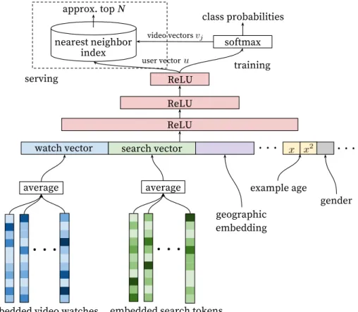
Digitalization brought us in a world where more and more of our decisions are taken in spite of in-formation overload. Recall that Negre (2015) defines recommender systems as "an inin-formation- information-filtering technique used to present the items of information (video, music, books, images, Web-sites, etc.) that may be of interest to the user." Recommender systems have consequently gained much traction as they help users navigating problems overcrowded with potential choices. They can be found almost everywhere, from booking a hotel room (e.g., with Booking.com (Bernardi et al., 2015)), a flat (e.g., with AirBnB (Haldar et al., 2019)), shopping online (e.g., on Ama-zon.com (Sorokina and Cantu-Paz, 2016)). . . to watching online videos (e.g., on YouTube (Cov-ington et al., 2016)) or films (e.g., on Netflix (Koren, 2009a)). This section provides a non-exhaustive overview of recommender systems to lay the ground on which we build algorithms well-suited to the challenges of the financial world.

(a) (b)

Figure 1.4: (a) Cumulative proportion of assets as a function of the cumulative proportion of RFQs, with assets ordered in descending order of activity. To avoid bias from expiring products, we only consider bonds alive in the whole period studied in this graph. We see that 80% of RFQs account for roughly 30% of the assets. (b) Histogram representing the number of unique clients interested in a particular asset. The x-axis shows the number of assets in the bucket corresponding to a specific number of unique clients. We see that a few assets are traded by lots of clients, whereas lots of assets were of interest for a small portion of the clients pool only. interest. Users can provide two sorts of feedback depending on the considered application: either an explicit or an implicit one. Explicit feedback corresponds to the ratings users give to items, such as a "thumbs up" on YouTube or a ten-star rating on IMDb. Implicit feedback corresponds to any feedback that is not directly expressed by users, such as a purchase history, a browsing history, clicks on links. . . : the interest of the user for the item is implied from her behavior. As explained in Section 1.1.1, our goal is to predict the future RFQs of BNPP CIB clients, given the RFQs they made and the RFQs made by everyone else. RFQs are also an example of implicit feedback: requesting the price of a product does not say anything about the client’s appeal for that product, or what the client ultimately chooses to do with it. As implicit feedback is our setting of interest in this thesis, we focus on it from now on.

In the implicit feedback setting, recommender systems can be understood as mappings f :

t, u, i _{≠æ x}t_ui, where t is a given time-step, u œ U is a given client, i œ I is a given product

and xt

uirepresents the interest of client u for product i at t. In most applications, the interest’s

dependence on time is ignored. xt

uiis usually interpreted either as a probability of interest or as

a score of interest, depending on the chosen mapping f. For a given client u, at a given t, the corresponding recommendation list is the list of all products ranked by their score in descending order, i.e., as 1xt_u(|I|≠i), iœ I2 with (·) the order statistics. For some real-world applications, e.g., YouTube (Covington et al., 2016), the cardinality of I prevents from computing scores for all i œ I and workarounds are used to compute scores for a relevant portion of items only. In our setting of interest, the cardinalities of both U and I allow for computing the scores of all

(client, product) pairs — we consequently focus on finding well-suited f mappings.

There are two recommender systems paradigms (Koren et al., 2009):

- Content-filtering. This approach characterizes clients and/or products through profiles, which are then used to match clients with relevant products and conversely. A classical formulation involves learning a mapping fu : t, i ≠æ xtui for each u œ U, with classic

supervised learning approaches where the items’ profiles are used as inputs to the fu’s.

al-ternative approach is to use a global mapping f : t, u, i ≠æ xt

ui using as input, e.g., a

concatenation of u and i profiles at t, and features depending on both u and i.

- Collaborative filtering. The term, coined by Goldberg et al. (1992) for Tapestry, the first recommender system, refers to algorithms making predictions about a given client using the knowledge of what all other clients have been doing. According to Koren et al. (2009), the two main areas of collaborative filtering are neighborhood methods and latent

factor models. Neighborhood methods compute weighted averages of the rating vectors

of users (resp. items) to find missing (user, item) ratings, e.g., using user-user (resp. item-item) similarities as weights. Latent factor models characterize users and items with vector representations of given dimension d inferred from observed ratings and use these vectors to compute missing (user, item) ratings. These two approaches can be brought together, e.g., as in (Koren, 2008).

Content- and collaborative filtering are not contradictory and can be brought together, e.g., as in Basilico and Hofmann (2004). Learning latent representations of users and items, as is done in latent factor models, has advantages beyond inferring missing ratings. These representations can be used a posteriori for clustering, visualization of user-user, item-item or user-item relationships and their evolution with time,. . . These applications of latent factors are particularly useful for business, e.g., to understand how BNP Paribas CIB clients relate to each other and consequently reorganize the way sales operate. For that reason, the collaborative filtering algorithms we study here are mainly latent factor models.

We now examine how baseline recommender systems can be obtained, develop on the content filtering approach with a specific formulation of the problem as a classification one, expand on some collaborative filtering algorithms and provide insights into other approaches for recom-mender systems.

1.3.1 Benchmarking algorithms

Baselines are algorithms that serve as reference for determining the performance of a proposal algorithm. Consequently, baselines are crucial for understanding how well an algorithm is doing on a given problem. In computer vision problems such as the ImageNet challenge (Russakovsky et al., 2015), the baseline is a human performance score. However, obtaining a human per-formance baseline is more complicated in recommender systems as the goal is to automate a task that is inherently not doable by any human: it would require at the very least an in-depth knowledge of the full corpus of users and items for a human to solve this recommendation task.

A simple recommender system baseline is the historical one. Using a classical train/test split of the observed events, a first baseline is given by the mapping fhist: (u, i) ≠æ ruiwith ruiœ N

the number of observed events for the (u, i) couple on the train split. The score can also be expressed as a frequency of interest, either on the user- or item-side; i.e., on the user-side as rui/qiœIrui. The historical model can also be improved using the temporal information,

considering that at a given t, closer interests should weigh more in the score. An example of such mapping is fhist : (t, u, i) ≠æ t≠1 ÿ tÕ₌₁ e≠⁄(t+1≠tÕ)rt_uiÕ (1.4) where rtÕ

ui denotes the number of observed events for the (u, i) couple at tÕ, and ⁄ is a decay

factor. Note that the sum stops at t ≠ 1 for prediction at t since observed events at t cannot be taken into account for predicting that time-step. In the following, we mainly use the most simple instance of baseline where the score of a (u, i) couple is given by their number of interactions observed in the training split.

1.3.2 Content-filtering strategies

We previously defined content filtering algorithms as mapping profiles of users, items, or both of them to the interest xt

ui. The difficulty of this approach lies in the construction of users and

items’ profiles, as they require data sources other than the observation of interactions between the two. As exposed in Section 1.2, we have at our disposal multiple data sources from which to build such profiles. Concretely, each of the three sources outlined in Section 1.2.1 leads to a profile — one can consequently build a user profile, an item profile, and an interaction profile from the available data.

The profile of a user (resp. item) is built from the numerical and categorical information available describing her (resp. its) state. Numerical features such as the buy/sell frequency of a user or the price of an item can be directly used. However, categorical features, e.g., the user’s country or the company producing the item, require an encoding for an algorithm to make use of them. Categories can be encoded in various ways, the most popular ones in machine learning being one-hot encoding, frequency encoding and target encoding. One-hot encoding converts a category c œ [[1; K]] to the c-th element ec of the canonical basis of RK,

ec= (0, . . . , 1, . . . , 0) œ RK, i.e., a zero vector with a 1 in the c-th position. Frequency encoding

converts a category c œ [[1; K]] to its frequency of appearance in the training set. Target encoding converts a category c œ [[1; K]] to the mean of targets y observed for particular instances of that category. One-hot encoding is a simple and widespread methodology for dealing with categorical variables; frequency and target encoding, to the best of our knowledge, could be more qualified of "tricks of the trade" used by data science competitors on platforms such as Kaggle (Kaggle Inc., 2020). One-hot encodings are, by essence, sparse and grow the number of features used by a model by as many categories there are per categorical feature. Deep learning models usually handle categorical features through embeddings, i.e., trainable latent representations of a size specifically chosen for each feature. These embeddings are trained along with all other parameters of the neural networks.

Provided with embeddings of categorical features describing the state of a particular user (resp. item), a profile of this user (resp. item) can be obtained by the concatenation of the numerical features and embeddings related to her. These profiles are then used to learn mappings fi

for all i œ I (resp. fu for all u œ U), or can be concatenated to learn a global mapping

f : (t, u, i) ≠æ xt

ui. One can also add cross-features depending on both u and i, such as the

frequency at which u buys or sells i. Indeed, in the financial context, it is usual for investors to re-buy or re-sell in the future products they bought or sold previously — cross-features describing the activity of a user u on an item i are consequently meaningful. A good practice for numerical features is to transform them using standard scores, as known as z-scores. A feature x is turned into a z-score z with z = x≠µ

‡ , where µ and ‡ are the mean and standard

deviation of x, computed using the training split of the data. Z-scores can also be computed on categories of a given categorical feature, using µcand ‡c for all c œ [[1; K]], provided that we have

enough data for each category to get meaningful means and variances. The distribution of a feature can vary much with categories: for instance, the buying frequency of a hedge fund is not the same as the one of a central bank. Using z-scores modulated per category of a categorical feature consequently helps to make these categories comparable.

In the implicit feedback setting, the recommendation problem can be understood as a classi-fication task. Provided with a profile, i.e., a set of features x describing a particular (t, u, i) triplet, we want to predict whether u is interested in i or not at t, i.e., predict a binary target

y _{œ {0, 1}. If, as mentioned in Section 1.1.1, we want to predict whether u is interested in}

buying and/or selling i, the target y can consequently take up to four values corresponding to a lack of interest, an interest in buying, in selling or in doing both, the last case happening only when the time-step is large enough to allow for it — the size of the time-step usually depends

on the liquidity of the considered asset class, as mentioned in Section 2.2.4. Classification is a supervised learning problem for which many classic machine learning algorithms can be used. A classic way to train a classifier is to optimize its cross-entropy loss, defined for a sample x as l(x) = ≠ C ÿ i=1 yi(x) log ˆyi(x) ,

a term derived from maximum likelihood where C is the total number of classification classes,

yi(x) = y(x)=i and ˆyi(x) the probability of class i outputted by the model for sample x. A

variation of cross-entropy, the focal loss (Lin et al., 2017), can help in cases of severe class imbalance. Focal loss performs an adaptive, per-sample reweighing of the loss, defined for a sample x as

lf ocal(x) = ≠

C ÿ i=1

(1 ≠ ˆyi(x))“yi(x) log ˆyi(x) , (1.5)

with “ an hyperparameter, usually chosen in the ]0; 4] range and depending on the imbalance ratio, defined in the binary case as the ratio of the number of instances in the majority class and the ones in the minority class. In imbalance settings, the majority class is easily learnt by the algorithm and accounts for most of the algorithm loss performance. The (1 ≠ ˆyi(x))“

term counterbalances this by disregarding confidently classified samples, and focuses the sum on "harder-to-learn" ones. Consequently, when the imbalance ratio is high, higher values of “ are favored.

The classifier can take many forms, from logistic regression (Hastie et al., 2009, Chapter 4) to feed-forward neural networks (Goodfellow et al., 2016). To date, one of the most widespread classes of algorithms is gradient tree-boosting algorithms (Hastie et al., 2009, Chapters 9,10). Popular implementations of gradient tree-boosting are XGBoost (Chen and Guestrin, 2016) and LightGBM (Ke et al., 2017). In a classic supervised learning setting with tabular data, these algorithms most often obtain state-of-the-art results without much effort. However, to handle time, these algorithms have to rely on hand-engineered features, as they only map a given input x to an output y. Instead of relying on hand-engineered features incorporating time, we could let the algorithm learn by itself how features should incorporate it using neural networks. Fawaz et al. (2019) provides a review of deep learning algorithms tackling time series classification. Two neural network architectures can be used to handle time series: recurrent neural networks, such as the Long Short-Term Memory (Hochreiter and Schmidhuber, 1997), or convolutional neural networks (see Appendix A.4). These networks map an input time series to a corresponding output one. For instance, in our case, we could use as input a series of features describing the state of a (u, i) pair at every considered time-step and as output the observed interest at that time. Convolutional neural networks are mostly used in visual recognition tasks. Their unidimensional counterpart used in natural language processing (NLP) tasks is, however, also appropriate for time series classification. WaveNet-like architectures (Oord et al., 2016), illustrated in Fig. 1.5, are particularly relevant to handle short- and long-term dependencies in time series through their causal, dilated convolutions.

Content-filtering is consequently a very diverse approach in terms of potential algorithms to use, as it can be seen as re-framing the problem of recommendation to the supervised learning task of classification. Its main shortcomings are linked to the usage of features. One needs to have features, i.e., external data sources, to build profiles, which is not a given in all recommender systems. Moreover, when profiling the (t, u, i) triplet, hand-engineering cross-features can lead to overfitting the historical data. An overfitted algorithm would then only recommend past interactions to a user: in most application cases, such recommendations are valueless for a user.

Because models with causal convolutions do not have recurrent connections, they are typically faster

to train than RNNs, especially when applied to very long sequences. One of the problems of causal

convolutions is that they require many layers, or large filters to increase the receptive field. For

example, in Fig. 2 the receptive field is only 5 (= #layers + filter length - 1). In this paper we use

dilated convolutions to increase the receptive field by orders of magnitude, without greatly increasing

computational cost.

A dilated convolution (also called `a trous, or convolution with holes) is a convolution where the

filter is applied over an area larger than its length by skipping input values with a certain step. It is

equivalent to a convolution with a larger filter derived from the original filter by dilating it with zeros,

but is significantly more efficient. A dilated convolution effectively allows the network to operate on

a coarser scale than with a normal convolution. This is similar to pooling or strided convolutions, but

here the output has the same size as the input. As a special case, dilated convolution with dilation

1

yields the standard convolution. Fig. 3 depicts dilated causal convolutions for dilations 1, 2, 4,

and 8. Dilated convolutions have previously been used in various contexts, e.g. signal processing

(Holschneider et al., 1989; Dutilleux, 1989), and image segmentation (Chen et al., 2015; Yu &

Koltun, 2016).

Figure 3: Visualization of a stack of dilated causal convolutional layers.

Stacked dilated convolutions enable networks to have very large receptive fields with just a few

lay-ers, while preserving the input resolution throughout the network as well as computational efficiency.

In this paper, the dilation is doubled for every layer up to a limit and then repeated: e.g.

1, 2, 4, . . . , 512, 1, 2, 4, . . . , 512, 1, 2, 4, . . . , 512.

The intuition behind this configuration is two-fold. First, exponentially increasing the dilation factor

results in exponential receptive field growth with depth (Yu & Koltun, 2016). For example each

1, 2, 4, . . . , 512

block has receptive field of size 1024, and can be seen as a more efficient and

dis-criminative (non-linear) counterpart of a 1 1024 convolution. Second, stacking these blocks further

increases the model capacity and the receptive field size.

2.2 S

One approach to modeling the conditional distributions p (x

| x

, . . . , x

)

over the individual

audio samples would be to use a mixture model such as a mixture density network (Bishop, 1994)

or mixture of conditional Gaussian scale mixtures (MCGSM) (Theis & Bethge, 2015). However,

van den Oord et al. (2016a) showed that a softmax distribution tends to work better, even when the

data is implicitly continuous (as is the case for image pixel intensities or audio sample values). One

of the reasons is that a categorical distribution is more flexible and can more easily model arbitrary

distributions because it makes no assumptions about their shape.

Because raw audio is typically stored as a sequence of 16-bit integer values (one per timestep), a

softmax layer would need to output 65,536 probabilities per timestep to model all possible values.

To make this more tractable, we first apply a µ-law companding transformation (ITU-T, 1988) to

the data, and then quantize it to 256 possible values:

f (x

) = sign(x

)

ln (1 + µ

|x

|)

ln (1 + µ)

,

3

Figure 1.5: The WaveNet architecture, using causal and dilated convolutions. Causal convolu-tions relate their output at t to inputs at tÕ_{Æ t only. Dilated convolutions, as known as à trous}

convolutions, only consider as inputs to a particular output index the multiples of the dilation factor at that index. Dilated convolutions extend the receptive field of the network, i.e., the period of time taken into account for the computation of a particular output. WaveNets used stacked dilated convolutions, with a dilation factor doubled up to a limit and repeated, e.g., 1, 2, 4, 16, 32, 1, 2, 4, 16, 32, . . . to get the widest receptive field possible. Illustration taken from Oord et al. (2016).

1.3.3 Collaborative filtering strategies

The collaborative filtering approach refers to algorithms using global information consisting of all observed (t, u, i) interactions to make local predictions about a given unobserved (t, u, i) triplet. As a matter of fact, recommendation tasks can be understood as predicting links in a bipartite graph Gt= (U, I, Et) with U the set of users, I the set of items and Etthe set of edges

connecting them, which may evolve with time depending on the studied problem. Et can be

summarized as an adjacency matrix At_{œ R}|U|◊|I| _{where a}t

ui= 1 if (u, i) œ Et, 0 else. When Et

evolves with time, the global information can be summarized in a three-dimensional, adjacency tensor A œ RT◊|U|◊|I| _{with T the total number of time-steps considered and A[t; u; i] = A}t_{[u; i].}

Note that At_{, and by extension A, is generally sparse, meaning that most of its entries are 0 —}

only a small portion of all the (u, i) couples are observed with a positive interaction. See Fig. 1.6 for an illustration of a bipartite graph and its associated adjacency matrix.

Figure 1.6: An example of bipartite graph and its associated adjacency matrix, where |U| = 3 and |I| = 5.

Consequently, one can think of collaborative filtering algorithms as learning to reconstruct the full adjacency matrix/tensor from an observed portion of it. We examine here algorithms that particularly influenced the work presented in this thesis. An extensive review of collaborative filtering can be found in (Su and Khoshgoftaar, 2009), and a survey of its extensions in (Shi

et al., 2014).

Matrix factorization and related approaches

Matrix factorization models learn to decompose the adjacency matrix into two matrices of lower dimension representing respectively users and items. For now, we disregard the influence of time, setting t = 0 and writing for convenience A := A0. A matrix factorization model learns

latent, sparse and lower-rank representations of users and items P œ R|U|◊d_{, Q œ R}|I|◊d _such

that

A¥ P QT (1.6)

with d an hyperparameter of the algorithm usually chosen as d π |U|, |I|. This equation is illustrated in Fig. 1.7. It follows that a given user u is mapped to a latent representation puœ Rd,

and a given item i respectively to qi œ Rd. The recommendation score of a given (u, i) couple

corresponds to the scalar product of their latent representations, xui= Èpu, qiÍ ¥ aui.

Figure 1.7: An illustration of the principle of matrix factorization in a recommendation frame-work.

A variation of matrix factorization, called nonnegative matrix factorization (NMF) (Paatero and Tapper, 1994; Hoyer, 2004) considers constraining the latent representations of users and items to nonnegative vectors. The motivation is twofold. First, in the implicit feedback setting, the matrix A is nonnegative itself, and it consequently makes sense to express it with matrices sharing the same constraint. Second, the latent factors can be understood as a decomposition of the final recommendation score, and a decomposition of an element in its latent components is generally expressed as a summation, from which an explanation can be derived — e.g., in (Hoyer, 2004) with the decomposition of face images in their parts (mouth, nose, . . . ) found using nonnegative matrix factorization. However, in a financial setting, latent factors are not explicit and cannot be conceptualized into meaningful components of a recommendation score. For that reason, the rationale behind NMF is usually dealt with a classic matrix factorization where scores are constrained to a given range, e.g., using the sigmoid function ‡(x) = 1/(1+e≠x₎

to map xui to [0; 1] in the implicit feedback setting.

Classic matrix factorization learns latent representations pu,’u œ U, qi,’i œ I by minimizing

the squared distance of the reconstruction P QT _{to the adjacency matrix A, computed on the}

set of observed scores Ÿ (Koren et al., 2009), as min p_ú,q_ú ÿ (u,i)œŸ 1 aui≠ qiTpu 22 + ⁄(ÎqiÎ2+ ÎpuÎ2) (1.7)

with ⁄ an hyperparameter controlling the level of L2-norm regularization. The parameters of this

least squares (Hu et al., 2008; Pilászy et al., 2010; Takács and Tikk, 2012). A probabilistic interpretation of this model (Mnih and Salakhutdinov, 2008) shows that this objective function is equivalent to a Gaussian prior assumption on the latent factors.

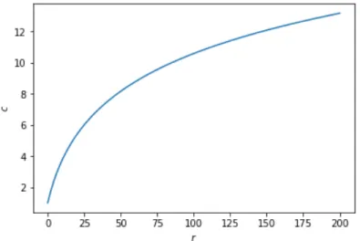
This formulation of matrix factorization is particularly relevant for explicit feedback. In implicit feedback however, all unobserved events are considered negative, and positive ones are implied — a (u, i) pair considered positive does not assuredly correspond to a true positive event, as explained in the incipit of this section. To counter these assumptions, Hu et al. (2008) introduce a notion of confidence weighing in the above equation. Keeping rui as the number of observed

interactions of the (u, i) pair in the considered dataset, the authors introduce two definitions of confidence:

- Linear: cui= 1 + –rui

- Logarithmic: cui= 1 + – log(1 + rui/‘)

where –, ‘ are hyperparameters of the algorithm. We empirically found logarithmic confidences to provide better results, a performance that we attribute to logarithms flattening the highly heterogeneous users’ and items’ activity we observe in our datasets (see Section 1.2.2). Defining

pui:= rui>0= aui, the implicit feedback objective is written

min pú,qú ÿ u,i cui 1 pui≠ qiTpu 22 + ⁄(ÎqiÎ2+ ÎpuÎ2). (1.8)

Note that the summation is now performed on all possible (u, i) pairs. Most often, the total num-ber of pairs makes stochastic gradient descent impractical, and these objectives are optimized using alternating least squares. In our case, however, the total number of pairs of a few millions — tens of millions, in the worst case — still allows for gradient descent optimizations.

A related approach is Bayesian Personalized Ranking (BPR) (Rendle et al., 2009), an optimiza-tion method specifically designed for implicit feedback datasets. The goal, as initially exposed, is to provide users with a ranked list of items. BPR abandons the probability approach for xui

used in the above algorithms to focus on a scoring approach. The underlying idea of BPR is to give a higher score to observed (u, i) couples than unobserved ones. To do so, the authors formalize a dataset D = {(u, i, j)|i œ I+

u · j œ I\Iu+} where Iu+ is the set of items which have

a positive event with user u in the considered data. D is consequently formed of all possible triplets containing a positive (u, i) pair and an associated negative item j. The BPR objective is then defined as maximizing the quantity

LBP R= ÿ

(u,i,j)œD

ln ‡(xuij) ≠ ⁄ Î Î2 (1.9)

where xuij is the score associated to the (u, i, j) triplet, defined such that p(i >u j| ) := xuij( )

with >u the total ranking associated to u — i.e., the ranking corresponding to the preferences

of u in terms of items, see Rendle et al. (2009, Section 3.1)—, and ⁄ is an hyperparameter controlling the level of regularization. As D grows exponentially with the number of users and items, this objective is approximated using negative sampling (Mikolov et al., 2013). Following matrix factorization ideas, we define xuij = xui≠ xuj, with xui= qTi pu where pu, qi are latent

factors defined as previously. The BPR objective is a relaxation of the ROC AUC score (see Section 1.4), a ranking metric also used in the context of binary classification. BPR combined with latent factors is, at the time of writing this thesis, one of the most successful and widespread algorithms to solve implicit feedback recommendation.

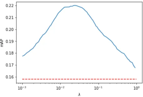
In specific contexts, Average Precision (AP) and the related mean Average Precision (mAP) are more reliable metrics than ROC AUC to score recommender systems — see Section 1.4 for an in-depth explanation of AP, mAP and a comparison of AP and AUC. Optimizing a relaxation