HAL Id: hal-02905874
https://hal.archives-ouvertes.fr/hal-02905874
Preprint submitted on 23 Jul 2020HAL is a multi-disciplinary open access archive for the deposit and dissemination of sci-entific research documents, whether they are pub-lished or not. The documents may come from teaching and research institutions in France or abroad, or from public or private research centers.
L’archive ouverte pluridisciplinaire HAL, est destinée au dépôt et à la diffusion de documents scientifiques de niveau recherche, publiés ou non, émanant des établissements d’enseignement et de recherche français ou étrangers, des laboratoires publics ou privés.
To Be or Not To Be a Verbal Multiword Expression: A
Quest for Discriminating Features
Caroline Pasquer, Agata Savary, Jean-Yves Antoine, Carlos Ramisch, Nicolas
Labroche, Arnaud Giacometti
To cite this version:
Caroline Pasquer, Agata Savary, Jean-Yves Antoine, Carlos Ramisch, Nicolas Labroche, et al.. To Be or Not To Be a Verbal Multiword Expression: A Quest for Discriminating Features. 2020. �hal-02905874�
To Be or Not To Be a Verbal Multiword Expression:
A Quest for Discriminating Features
Caroline Pasquer University of Tours
France
Agata Savary, Jean-Yves Antoine University of Tours
France
Carlos Ramisch
Aix Marseille Univ, Universit´e de Toulon, CNRS, LIS, Marseille, France [email protected]
Nicolas Labroche, Arnaud Giacometti University of Tours
France
Abstract
Automatic identification of mutiword ex-pressions (MWEs) is a pre-requisite for semantically-oriented downstream applica-tions. This task is challenging because MWEs, especially verbal ones (VMWEs), exhibit sur-face variability. However, this variability is usually more restricted than in regular (non-VMWE) constructions, which leads to various variability profiles. We use this fact to deter-mine the optimal set of features which could be used in a supervised classification setting to solve a subproblem of VMWE identifica-tion: the identification of occurrences of pre-viously seen VMWEs. Surprisingly, a sim-ple custom frequency-based feature selection method proves more efficient than other stan-dard methods such as Chi-squared test, infor-mation gain or decision trees. An SVM classi-fier using the optimal set of only 6 features out-performs the best systems from a recent shared task on the French seen data.
1 Introduction
Multiword expressions (MWEs) are word combi-nations with idiosyncratic characteristics regard-ing for instance morphology, syntax or seman-tics (Baldwin and Kim, 2010). One of their most emblematic properties is semantic non-compositionality: the meaning of the whole expression cannot be straightforwardly deduced
from the meaning of its components, as in to cut corners ‘to do an incomplete job ’1. Due to this property, as well as to their pervasiveness ( Jack-endoff, 1997), MWEs constitute a major chal-lenge for semantically-oriented downstream appli-cations, such as machine translation, information retrieval or sentiment analysis. A prerequisite for an appropriate handling of MWEs is their auto-matic identification.
MWE identification aims at automatic location of MWEs in running text. This task is very chal-lenging, as signaled by Constant et al. (2017), and further confirmed by the PARSEME Shared Task on automatic identification of verbal MWEs (Ramisch et al.,2018). One of the main difficulties stems from the variability of MWEs, especially verbal ones (VMWEs). Namely, even if a MWE has previously been observed (in a training corpus or in a lexicon), it can re-appear in morphosyn-tactically diverse forms, where components vary inflectionally, their order is inverted, discontinu-ities occur and syntactic relations change between lexicalized components, as in examples (1–2).
(1) Some companies were cutting cornersOBJto save costs. (2) The field would look uneven if cornersSUBJwere cut.
1Henceforth, the lexicalized components of a MWE,
i.e. those always realized by the same lexemes, appear in bold.
However, assuming unrestricted variability is not a good strategy either, since it may lead to literal or coincidental occurrences of MWEs’ components, as in (3) and (4).2
(3) Start withcutting one::::: :::::corner of the disinfectant bag. (4) If youcut along this line, you’ll get an acute:: :::::corner.
To tackle these challenges, we focus on a subprob-lem of MWE identification (henceforth referred to as the Task), namely the identification of previ-ously seen VMWEs.
We deal with French, which exhibits a partic-ularly rich verbal inflection, and whose VMWE-annotated corpus is one of the richest PARSEME Shared Task benchmark datasets. However, the proposed methods are language-independent in that they rely on universal properties of VMWEs and feature sets. Our aim is to determine the opti-mal set of features which would allow us to auto-matically discriminate between VMWEs and non-VMWEs in a supervised classification framework. To this aim, we first study the linguistic properties of VMWEs which may serve as a basis for defin-ing the initial set of features (Sec.2). Then, we describe the corpora used for training and evalu-ation (Sec. 3). Further, we address the selection of the positive/negative candidates from the cor-pus (Sec.4). We discuss the successive phases of feature selection (Sec.5): the definition of the ini-tial set of features; the ranking of these features by their relevance to the task; and establishing the optimal number of best-ranked features by off-the-shelf binary classifiers. Then, the results are discussed (Sec. 6) and we interpret some of the selected features from a linguistic point of view (Sec.7). Finally, we conclude and suggest direc-tions for future work (Sec.8).
2 Linguistic properties of VMWEs The major observation underlying our work is that VMWEs are mostly morphosyntactically regular at the level of tokens (individual occurrences) but idiosyncratic at the level of types (sets of surface realizations of the same expression). For instance, considering the VMWE type to cut corners in-stantiated by the VMWE tokens in (1) and (2), we find no ”surface” (i.e. non-semantic) hints that distinguish them from regular English verb-object constructions (e.g. cut branches). They respect standard grammar rules (the object follows the
2Henceforth, literal and coincidental occurrences are
highlighted with wavy underlining.
verb; in passive, the verb occurs in participle, etc.). Unlike named entities, they use no capitalisation and contain no trigger words. However, number inflection of the noun is prohibited by this VMWE, i.e. using the noun in singular leads to the loss of the idiomatic meaning, as shown in example (3). This is in contrast to regular verb-object construc-tions (cut a branch ), in which noun inflection does not significantly change the overall meaning.
Such a restricted variability of MWEs is one of their fundamental properties, as argued in linguis-tic work (Gross,1988;Nunberg et al.,1994;Tutin,
2016;Sheinfux et al.,2018). Namely, a given syn-tactic structure in a given language comes with a set of various morphosyntactic variations con-sidered grammatical (e.g. English transitive verb constructions admit passivisation, noun inflection, pronominalisation, etc.). But a MWE of the same structure usually allows only a proper subset of these variants, which we will call its variability profile. These profiles are numerous and hard to predict, e.g. while cut corners admits pas-sivisation but prohibits number inflection, build bridges ‘establish links’ accepts both of these variants, and take place ‘happen’ none of them.
Studying variability profiles in corpora is hindered by another fundamental property of VMWEs – their Zipfian distribution: few VMWE types occur frequently in corpora, and there is a long tail of VMWE types occurring rarely.
The third property we are interested in is the fact that some VMWE types do share common ”surface” properties, e.g. most light-verb constructions have no lexicalized de-terminers (take a/many/several/no break(s) ) and contain frequent light verbs (e.g. take a walk/break/advantage/etc.). These shared prop-erties, however, are rarely semantically motivated: VMWEs exhibit a strong lexical inflexibility, i.e. replacing a lexicalized component with a semantically close word (a synonym, hyperonym, etc.) usually results in the loss of the idiomatic reading, in example (5), as opposed to (1–2).
(5) The field would look uneven if borders were reduced.
In this work, we hypothesize that: (i) variability profiles of VMWEs, materialized by morphosyn-tactic features in annotated corpora, can help correctly identify occurrences of previously seen VMWEs, (ii) for rarely occurring VMWEs, their resemblance with other, more frequent, VMWEs can also help solve the Task. The two
hypothe-ses give rise to relative and absolute features, de-scribed in Sec.5.1.
3 Corpus
In 2018, edition 1.1 of the PARSEME Shared Task, henceforth PST (Ramisch et al.,2018), took place, with a goal of boosting the development of identifiers for both seen and unseen VMWEs. To this end, a corpus of verbal MWEs was manually annotated and openly published for 19 languages.3 We use the French part of this corpus, and we refer to its particular subcorpora as TrainST and TestST, which reflects their function in PST.
In our experiments, TrainST is used: (i) for training and testing during feature selection (Sec. 4–5), (ii) for training during the evalua-tion of the final system against the PST results (Sec.6.2), and prior to the extraction of candidates for manual evaluation on a large external corpus (Sec.6.3). TestST is only used as a testing bench-mark in the PST evaluation setting (Sec.6.2).4
For manual evaluation (Sec. 6.3), we also use a large corpus collected from Wikipedia and by webcrawling for the CoNLL 2017 Shared Task.5
It is automatically segmented, tokenized and morpho-syntactically annotated (Zeman et al.,
2018) but it does not contain VMWE annotations. Tab. 1 shows the statistics of the 3 corpora, in terms of the number of sentences, tokens, all annotated VMWEs and those annotated VMWEs which also occur in TrainST (the Task is limited to them).
All corpora comply with the CoNLL-U format6, i.e. contain, for each surface form, its lemma, POS, morphological features and syntactic depen-dencies.
VMWEs are manually annotated and catego-rized into: verbal idioms (VID: cut corners), light-verb constructions (LVC: take a walk ), in-herently reflexive verbs (IRV: s’apercevoir ‘to perceive oneself ’⇒‘to realize’) and multi-verb constructions (MVC: to make do). Thus, contrary to other works which focus on verb-noun VMWEs (Fazly et al., 2009), we handle various syntactic profiles. Note, however, that the Task only ad-dresses VMWE identification and abstracts away from categorisation.
3
http://hdl.handle.net/11372/LRT-2842
4
In the PST corpus, there is also a small development cor-pus for French, which we do not use.
5
http://hdl.handle.net/11234/1-1989
6
http://universaldependencies.org/format.html
Corpus # Sentences # Tokens # VMWEs # Seen TrainST 17,225 432,389 4,550 4,550100%
TestST 1,606 39,489 498 251 50%
CoNLL 306,431,406 5,242,235,570 n/a n/a Table 1: Statistics about corpora. Seen refers to those VMWEs which also appear in TrainST.
4 Candidate extraction
In order to test the hypotheses put forward in Sec. 2, we propose a supervised classification method for identifying previously seen VMWEs.
In the first step, we design a procedure, hence-forth called ExtractCands, to extract VMWE candidates. It will be employed in: (i) training, to choose positive and negative VMWE examples, further used for feature selection, (ii) testing, for pre-identifying VMWE candidates to be fed to the classifier. For every VMWE e attested in the train-ing corpus, ExtractCands extracts each co-occurrence c of e’s lexicalized components, pro-vided that the following conditions are fulfilled.
First, the sets of lemmas and parts-of-speech of e’s and c’s components are identical. For instance, for e in (6), the candidate in (7) will be extracted but not the one in (8), due to the different POS of mesure ‘measure’.
(6) Il prendVERBplusieursDETmeasuresNOUN. ’He takes sev-eral measures.’
(7) Je prendsVERBuneDETmesureNOUNunconstitutionnnelle. ’I take an unconstitutional measure.’
(8) Il
::::
prendVERB une r`egle et
:::::
mesureVERB la longueur. ’He takes a ruler and measures the length.’
Second, if c contains two components or if there is only one verb and one noun, they must be either directly connected in the syntactic depen-dency tree or separated by only one element. This condition is fulfilled (7) and in case of complex determiners as in Fig.1(a), but not in coinciden-tal occurrences like in Fig.1(b). No dependency constraints were defined for candidates with more than two components due to their lower frequency and to computational constraints.7
Third, based on c’s discontinuities seen in TrainST, we restrict the number of external ele-ments that can be inserted between c’s compo-nents, to avoid large numbers of spurious candi-dates stemming from frequent lemmas (e.g. deter-miners or pronouns), as in (9).
7Searching for existing, direct or indirect, dependencies
between pairs taken from up to 7 components would be time-consuming.
(a) Il prend une série de mesures inconstitutionnelles. He takes a series of measures unconstitutional.
obj nmod
(b) Ces :::::::mesures seront améliorées et on promet d’en:::::::prendre d’autres en compte.
These measures will be enhanced and one promises to take others into account.
subj conj xcomp
Figure 1: VMWE candidates with discontinuous dependency chains: (a) extracted, (b) non-extracted.
Corpus Extracted candidates P R
All Positive Negative
TrainST 4,596 3,582(78%) 1,014(22%) 0.78 0.98
TestST 368 210(57%) 158(43%) 0.57 1.00
CoNLL 32,789,815 n/a n/a n/a n/a Table 2: Results of candidate extraction, based on at-tested VMWEs seen at least twice in TrainST.
(9) Ilfaut rappeler que, jusqu’en 1983,:: il n’y avait pas . . .: One must remind that, until 1983, there was no . . .
Finally, since we wish to test the variability profile hypothesis (Sec. 2), we retain only those VMWEs whose number of occurrences is high enough to be representative of their variability. However, this frequency threshold cannot be too high, otherwise the size of the annotated data would dramatically drop. For a reasonable trade-off between these two factors, we select only those candidates whose attested VMWEs appear at least twice in the training corpus (3582 occurrences i.e. 78% of TrainST).
When ExtractCands is used for training, the extracted candidates are marked as positive, if they are manually annotated as VMWEs in TrainST, and negative otherwise. Tab.2shows the results of the candidate extraction in the corpora from Tab.1. As expected, the method is tuned for a high re-call and a reasonable precision. The latter factor should grow due to classification, based on a care-fully selected set of features, which is addressed in the following section.
5 Feature selection
In supervised classification, the VMWE candi-dates to classify are to be represented by sets of features. The choice of such features is crucial for the quality of the classification outcome and its ad-equacy for the tested hypotheses. This section de-scribes the initial set of features and the selection of those which are the most relevant to the Task. 5.1 Initial set of features
As discussed in Sec. 2, we hypothesize that the variability profiles of VMWEs can help correctly identify occurrences of previously seen VMWEs. Representing these profiles straightforwardly is
not always easy (e.g. for passivization or pronom-inalization), especially in a language-independent way. But, we assume that they can be approxi-mated by simpler properties directly encoded in the CoNLL-U files (Sec. 3). Thus, our start-ing point is a set of features related to morphol-ogy, syntax and insertions. Morphological fea-tures mostly refer to verb or noun inflection. Syn-tactic features relate to dependency relations out-going from a component (e.g. subject vs. object) or to the fact that the components are syntacti-cally (in)directly connected. Insertion-bound fea-tures account for the number of words inserted be-tween the lexicalized components, e.g. 2 insertions in (10), and to their POS sequence, e.g.DET ADJ
in (10). Insertions and syntactic dependencies may convey similar information, e.g. in (10) the adjec-tive is accounted for both as an insertion and as a modifier of the noun. But they may also be com-plementary, as in (11), since syntactic dependen-cies capture modifiers not included between the lexicalized components.
(10) Il prend d’DETimportantesADJmesures ’He takes ∅DET important measures’
(11) Il prend desDET mesures aussi (voire de plus en plus) importantesADJ ‘He takes as (or even more and more) important measures’
Recall (Sec.2) that the variability profile is de-fined on the level of VMWE types rather than to-kens. This is why, followingPasquer et al.(2018), we put strong impact on relative features. Namely, given a VMWE candidate c, and its reference VMWE token together with all attested VMWE tokens of the same type ({e1, e2, . . . , en}), we
compare the properties of c to those of ei (1 ≤
i ≤ n). Relative features always take binary val-ues. Thus, the REL INSERTSEQ feature is true if the POS sequence of the words inserted between c’s components is the same as in any ei, as in (7)
vs. (6), and false otherwise, as in (11) vs. (10). Also, REL SYNTACTICDEPENDENCIES VERB is true if the set of dependency relations outgoing from the verb in c is the same as in any ei, and
false otherwise, etc.
Recall that VMWEs have a Zipfian distribution, thus relative features may be unreliable for many VMWE types occurring rarely. Thus, we also use
absolutefeatures. They are similar to the relative ones, but they are categorical rather than binary. For instance, the value of ABS INSERTSEQis the POS sequence of the inserted words, e.g.DET ADJ
in (10). Absolute features also include the VMWE set of lemmas, e.g. {mesure, prendre}, and their categorization (e.g. LVC).
Note finally that no word embeddings are used in the initial set of features. This is justified by lexical inflexibility of VMWEs: a new VMWE can rarely be discovered by semantic similarity of its components to those of attested VMWEs. This observation is confirmed by the PST, where best VMWE identifiers, even those using word embed-dings, never exceed F-measure of 0.28 for unseen VMWEs. In our opinion, this very weak gener-alisation power should be approached by system-atically coupling VMWE identification with their automatic discovery, which our perspective for fu-ture work.
5.2 Usefulness of automatic feature selection The initial set of relative and absolute features de-fined in the previous section is huge: with the UD tagset used in our corpora, we get 18,000 possible features in total. If we only keep those features which are activated at least once in the corpus, this number is reduced to about 800. The ques-tion is then how to select those features which are the most discriminating for the Task.
Most systems from PST use features which are known to be linguistically relevant, and which are relatively simple to calculate (Waszczuk, 2018;
Taslimipoor and Rohanian,2018;Boros and Bur-tica, 2018; Stodden et al., 2018; Moreau et al.,
2018,?;Berk et al.,2018;Ehren et al.,2018; Pas-quer et al.,2018;Zampieri et al.,2018).8
Another approach was to feed all/most poten-tially relevant features to the classifier and let it de-termine the appropriate weights for those features (Pasquer et al.,2018). In this work, we also rely on domain knowledge to define the initial set of fea-tures, but we use automatic feature selection meth-ods. The motivation is threefold. First, a lower number of accurately chosen features should lead to classification of a higher quality and shorter training time. Second, we might discover features whose relevance to the Task has not been linguis-tically established. Third, automatic procedure is
8A summary of this state of the art is offered in the
Ap-pendix B.
language-independent, as soon as the initial set of features is generic enough.
The feature selection process runs in two stages: (i) feature ranking, (ii) choice of the optimal num-ber of the best-ranked features.
5.3 Feature ranking
We experimented with 4 feature ranking methods described below. All but the first require annotated data and are applied to the TrainST corpus. FREQ This is a custom frequency-based method. We apply the ExtractCands from Sec.4to the CoNLL corpus, which yields 2.6 million candi-dates.9 Then, we select only those feature-value pairs which appear in at least one candidate, and we rank them by decreasing frequency. Finally, we strip the values and only keep the features.10 CHI2 The Chi-squared test (Kumbhar and Mali,
2016) looks at candidates having both the given feature-value pair f v and the given class cl. It cal-culates the difference between their observed and expected frequencies, under the hypothesis that f v and cl are independent. We use the Pearson’s ver-sion of this test, and the feature-value ranking cor-responds to decreasing chi-squared value. We fi-nally strip the values, as in FREQ.
GAINThe information gain (Kumbhar and Mali,
2016) method partitions the set of observations ac-cording to different values of a given feature f , calculates the weighted sum of the entropies of these partitions, and compares it to the entropy of the whole set. If the entropy strongly drops after the partition, the information gain is high, i.e. f is strongly discriminating. The feature ranking cor-responds to the decreasing value of the gain. FORESTThe Random Forest algorithm (Breiman,
2001), combines many decision trees (here: 10 trees with no depth limit) into a single model by a majority or weighted vote. For the construction of the tree, the quality of each split is measured by the Gini impurity. Features are then ranked by their relevance when determining splits.
5.4 Tuning the number of features
Each of the methods from the previous section ranks the initial set of features according to their estimated relevance to the Task. We now need to
9Their classes are unknown, since the CoNLL corpus in
not annotated for VMWEs.
10After stripping, features may have several occurrences,
corresponding to different values. We only keep the occur-rence with the highest rank.
decide how many best-ranked features from each ranking should be selected. We tune this parame-ter with 3 standard supervised classification meth-ods – Naive Bayes, linear SVM and decision trees – using their off-the-shelf implementations.11
For each classifier C, and for each feature rank-ing list R from Sec.5.3, we proceed by a greedy method : (i) we select the i best-ranked features from R, (ii) we train and test C, with the i selected features, in a 10-fold unstratified cross-validation setting with a 90%-10% split of the TrainST cor-pus, where the candidates for both training and testing are those extracted by ExtractCands, (iii) we calculate the mean F-measure Fmean for
the 10 folds, (iv) we repeat steps (i–iii) for every i from 1 to length(R) and we select the value of i for which Fmeanis the highest.
6 Results
In this section we show the results of the feature selection process described above. Then, we eval-uate the obtained set of features by two meth-ods: by the comparison of the best-performing classifier-selection pair to benchmark results, and by a manual evaluation of the same pair on an ex-ternal large corpus.
6.1 Optimal feature sets
Tab. 3 shows the best results (i.e. the results for the optimal number of best-ranked features) of the feature selection experiments described in Sec.5, for the 4 feature ranking methods and the 3 classi-fiers. P , R and F are the mean scores from the 10 folds, and σ is the variance of the 10 F-scores.12
Surprisingly, FREQ, which is a custom method, initially conceived to only remove irrelevant fea-tures from the initial set, achieves identical or bet-ter results than standard feature selection methods, with F = 0.936 for the linear SVM.
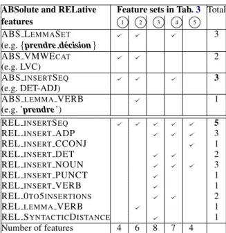
The optimal feature sets corresponding to these results are described in Tab. 4. There is a no-table consistence in the optimal sets selected by each method. For CHI2, GAIN and FOREST, each of the 3 classifiers selects always the same set
11NLTK (Loper and Bird, 2002) for Naive Bayes, and
Scikit-learn (Pedregosa et al.,2011) for SVM and decision trees.
12
The low value of variance indicates that the simple 90%-10% corpus split method is sufficiently reliable. If variance were higher, stratified validation would be more appropriate (i.e. the corpus would have to be split in such a way that the proportion of data belonging to each class is the same in each fold as in the whole corpus).
FeatSelectFeature setClassif P R F σ 1 NB 0.8810.9650.9210.012 FREQ 2 SVM 0.8960.9800.9360.015 Dec. Tree 0.9130.9340.9230.009 NB 0.8180.9750.8890.011 CHI2 3 SVM 0.8260.9730.8930.013 Dec. Tree 0.8330.9640.8940.012 NB 0.8260.9740.8940.013 GAIN 4 SVM 0.8970.9800.9360.015 Dec. Tree 0.8750.9620.9160.020 NB 0.7870.9750.8710.016 FOREST 5 SVM 0.7870.9750.8710.016 Dec. Tree 0.7870.9750.8710.016 Table 3: Best mean performance on 10% of TrainST (in 10 cross-fold validation). The feature sets are detailed in Tab.4.
ABSolute and RELative Feature sets in Tab.3 Total
features 1 2 3 4 5
ABS LEMMASET 3
(e.g. {prendre,d´ecision}
ABS VMWECAT 2
(e.g. LVC)
ABSINSERTSEQ 3
(e.g. DET-ADJ)
ABSLEMMAVERB 1
(e.g. ’prendre’)
RELINSERTSEQ 5
RELINSERT ADP 3
RELINSERT CCONJ 1
RELINSERT DET 2
RELINSERT NOUN 3
RELINSERT PUNCT 1
RELINSERT VERB 1
REL 0TO5INSERTIONS 2
RELLEMMAVERB 1
REL SYNTACTICDISTANCE 1
Number of features 4 6 8 7 4
Table 4: Optimal feature sets mentioned in Tab.3
(resp. 3 , 4 , 5 ). For FREQ, the two sets ( 1 and 2 ) vary by one feature only. However, the sets are quite diverse from one selection method to another, which proves the complementarity of the methods.
The optimal number of features varies from 4 to 8. As expected, relative features are more often selected; CHI2 and FOREST select even exclu-sively relative features. This is consistent with our variability-profile hypothesis (Sec.2). One feature (REL INSERTSEQ) is selected by all methods, and there are 6 features selected only once.
6.2 Benchmark evaluation
It is interesting to evaluate the quality of the fea-ture set selection by a direct comparison to the 17 systems having participated in the PST cam-paign (cf. Sec. 3). PST defined evaluation mea-sures which are specific to phenomena constitut-ing known challenges in VMWE identification. One of them is the seen-in-train score, i.e. the P/R/F calculated only for those VMWEs in TestST which were previously seen in TrainST. In PST, a VMWE from TestST is considered seen if a VMWE with the same (multi-)set of lemmas is an-notated at least once in TrainST.
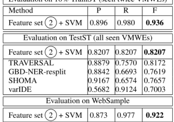
We compare our optimal 2 +SVM classi-fier with the PST results for French13 as fol-lows: (i) SVM is trained on the whole TrainST corpus (with ExtractCands and feature set 2 ), (ii) we apply it to the candidates extracted with ExtractCands from TestST, (iii) those VMWEs from TestST which were either omitted by ExtractCands or wrongly classified simply count as false negatives. This obviously lowers the results as compared to Tab.3, where only the VMWEs seen at least twice are considered.
As shown in Tab.5, the F-measure of 2 +SVM indeed drops by over 11 points in the PST setting (to 0.8207). However, this is much higher than F = 0.7003 obtained by varIDE (Pasquer et al.,
2018) with a quite similar method, except that, there, only Naive Bayes with no feature selection is used. This highlights the fact that focusing on a small set of relevant features helps the classifi-cation. What is more, our F-measure is slightly higher than the best registered F-score (0.8172) by TRAVERSAL (Waszczuk,2018), where logis-tic regression is applied to sequences of nodes in dependency trees. Additionally, the handling of the variant-of-train VMWEs (i.e. those VMWEs in TestST which appear with a different surface form than in TrainST) is better with our method than with TRAVERSAL (F = 0.7317 vs. 0.7123). We also get better seen-in-train F-scores than the second and third best systems, based on neural networks: GBD-NER-resplit (Boros and Burtica,
2018), which only uses the provided PST corpora, and SHOMA (Taslimipoor and Rohanian, 2018), which also employs Wikipedia word embeddings. When 2 +SVM is evaluated on all VMWEs from the French TestST, not only the seen ones,
13
https://gitlab.com/parseme/sharedtask-data/tree/ master/1.1/system-results
Evaluation on 10% TrainST (seen twice VMWEs)
Method P R F
Feature set 2 + SVM 0.896 0.980 0.936 Evaluation on TestST (all seen VMWEs) Feature set 2 + SVM 0.8207 0.8207 0.8207 TRAVERSAL 0.8879 0.7570 0.8172 GBD-NER-resplit 0.8842 0.6693 0.7619 SHOMA 0.9167 0.6574 0.7657 varIDE 0.5682 0.9124 0.7003 Evaluation on WebSample Feature set 2 + SVM 0.873 0.977 0.922
Table 5: Evaluation results in the PST benchmark set-ting, and with a manually annotated external corpus
the F-score decreases to 0.55, which is still rela-tively close to 0.56 obtained by the best system (TRAVERSAL), even if unseen VWMES are to-tally beyond the scope of our work.
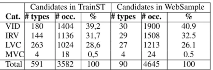
6.3 Manual evaluation on an external corpus It is also interesting to evaluate the quality of the selected feature set on an external corpus, inde-pendent of the one used for the selection. To this end we constructed a representative sample of the CoNLL corpus, called WebSample, that could be manually checked. Namely, WebSample should respect the distribution observed in TrainST, as far as frequencies of VMWEs and of their categories are concerned. To this aim, we first checked the proportion of the 4 categories (VIDs, LVCs, IRVs and MVCs) in the VMWEs seen at least twice in TrainST. Then, we selected 90 VMWE types
14 in such a way that these proportions are
re-spected (except for MVCs, which are very rare in TrainST) and that VMWEs types in each category have high, low and median frequency (with a bal-anced distribution). For MVCs, we selected all 4 VMWE types appearing in TrainST. Finally, the 90 VMWE types selected in TrainST were given as the reference set to ExtractCands, which was then applied to the CoNLL corpus. The re-sulting set of candidates was trimmed so that equal numbers of candidates come from the Wikipedia and the webcrawling part of the CoNLL corpus.
Tab. 6 shows the outcome of this procedure. The resulting set of 4645 candidates (from 90 types), together with their occurrence contexts, was then manually annotated by 4 experts. 27 occurrences (0.6%) were eliminated due to
Candidates in TrainST Candidates in WebSample Cat. # types # occ. % # types # occ. %
VID 180 1404 39,2 30 1900 40.9
IRV 144 1136 31,7 29 1508 32.5
LVC 263 1024 28,6 27 1213 26.1
MVC 4 18 0,5 4 24 0.5
Total 591 3582 100 90 4645 100
Table 6: WebSample w.r.t. TrainST (VMWEs seen at least twice) VMWE category P R F VID 0.917 0.961 0.939 IRV 0.873 0.985 0.926 LVC 0.830 0.990 0.903 MVC 0.750 0.750 0.750 All 0.873 0.977 0.922
Table 7: SVM results on WebSample per category
rect sentences, errors (POS, lemma), non-French words or insufficient context. This low rejec-tion rate confirms the good overall quality of the CoNLL corpus. The 4618 remaining candidates were manually labelled as positive (68.7%) and negative.
The WebSample corpus was then used as the testing corpus for our 2 +SVM classifier. As shown in Tab. 7, we obtained the overall F-measure of 0.922, which is comparable to the 0.936 achieved on TrainST and highlights the good repeatability of the method whatever the cor-pus: our system suffers neither from overfitting nor from sensitivity to the data source. As to per-category results disregarding the MVCs (whose number is negligible), LVCs are the hardest to classify (F = 0.903), probably due to their high variability, as illustrated in examples (12–16). 7 Linguistic relevance of the selected
features
The selected features prove relevant to the phe-nomenon of VMWE variability. First, as outlined in Tab. 4, the inserted POS sequences like DET ADJin (14) always stand at the top of feature rank-ings (as a REL and/or an ABS feature), whereas this feature is generally not taken into account in other works. Insertions can, indeed, model many relevant phenomena such as the determiner flexi-bility in (12) vs. (13), allowed modifiers as the ad-jective in (14), passivization (15) or relativization (16). Inserted POSes including VERB, NOUN or PUNCTuation appear as the most relevant, maybe because they may suggest a non-VMWE as in I
::::
build viaductsNOUN, you constructVERB:::::::bridges.
(12) Je prends desDETd´ecisions ‘I make decisions’ (13) Je prends deuxNUMd´ecisions ‘I make two decisions’ (14) Je prends uneDET grandeADJ d´ecision ‘I make a great
decision’
(15) Ma d´ecision estAUXprise ‘My decision is made’ (16) C’est la d´ecision quePRONjePRONprends ‘It is the
deci-sion I make’
Note that 3 of the 6 selected features are lexical: they relate to the lemmas of the VMWE com-ponents. Without these features, our F-score de-creases by 4 points. This confirms the strength of the lexical inflexibility phenomenon (Sec. 2) and the hardness of generalization over unseen data, observed in PST.15
Some features, considered relevant to VMWE variability, do not appear as selected in Tab. 4. E.g. many VMWEs prohibit the modification of the noun (to:::cut acutecorners) or its inflection for:::::: number (tocut a:: corner). Given that such varia-::::: tions are often tolerated by LVCs but not by VIDs, the VID candidates may not have been sufficiently numerous to acquire such knowledge about VID constraints.
8 Conclusions and future work
We presented a methodology for selecting a rel-evant set of features which can be used in a supervised classification framework to solve the task of identifying occurrences of previously seen VMWEs. It is based on defining an initial large set of linguistically-motivated features, and then ap-plying 4 feature selection methods, together with 3 classifiers, to select the optimal sets of features.
The results show that relative features (those re-flecting the variability profiles of VMWEs) domi-nate in the optimal selections. Most of the selected features are based on the properties of external in-sertions. Such features are never or rarely explic-itly considered in previous works.
In sum, our system’s main contributions are: (i) its performances, on par, for French, with the best systems of a recent shared task, (ii) its abil-ity to highlight linguistic properties of VMWEs by a novel combination of features, (iii) its inter-pretability and classification efficiency due to only 6 features, (iv) its generalization power confirmed by an evaluation on an external large corpus.
The fact that 50% of the optimal features are lemma-based stresses the lexical nature of the
15The best average PST results limited to unseen data are
below F = 0.29, even for systems using neural networks and word embeddings (Ramisch et al.,2018).
MWE phenomenon, which implies the particu-larly acute hardness of generalising over unseen data. We believe that this hardness cannot be over-come by more powerful features (e.g. stemming from distributional semantics), but should rather be handled by coupling MWE identification with unsupervised MWE discovery. In this way, large parts of the unseen data can be transformed into seen data, and their corpus occurrences can com-plement the manually annotated training corpus. We will address such coupling in future work.
Other perspectives include a detailed error anal-ysis as well as finding strategies for VMWEs seen once, which were disregarded here. The rele-vant features likely differ among different VMWE classes, since these classes have different syntac-tic properties. Therefore, it should be useful to perform the feature selection separately for each class. Finally, we could evaluate the genericity of our method by evaluating it on other languages of the PARSEME Shared Task. The feature selection across languages or language families might, in-deed, reveal universal characteristics of VMWEs.
References
Timothy Baldwin and Su Nam Kim. 2010. Multiword expressions. In Nitin Indurkhya and Fred J. Dam-erau, editors, Handbook of Natural Language Pro-cessing, 2 edition, pages 267–292. CRC Press, Tay-lor and Francis Group, Boca Raton, FL, USA. G¨ozde Berk, Berna Erden, and Tunga G¨ung¨or. 2018.
Deep-BGT at PARSEME Shared Task 2018: Bidi-rectional LSTM-CRF model for verbal multiword expression identification. In Proceedings of the Joint Workshop on Linguistic Annotation, Multi-word Expressions and Constructions (LAW-MWE-CxG-2018), pages 248–253.
Tiberiu Boros and Ruxandra Burtica. 2018. GBD-NER at PARSEME Shared Task 2018: Multi-word expression detection using bidirectional long-short-term memory networks and graph-based decoding. In Proceedings of the Joint Workshop on Linguistic Annotation, Multiword Expressions and Construc-tions, LAW-MWE-CxG@COLING 2018, Santa Fe, New Mexico, USA, August 25-26, 2018, pages 254– 260. Association for Computational Linguistics. Leo Breiman. 2001. Random forests. Machine
Learn-ing, 45(1):5–32.
Mathieu Constant, G¨uls¸en Eryi˘git, Johanna Monti, Lonneke van der Plas, Carlos Ramisch, Michael Rosner, and Amalia Todirascu. 2017. Multiword ex-pression processing: A survey. Computational Lin-guistics, 43(4):837–892.
Rafael Ehren, Timm Lichte, and Younes Samih. 2018. Mumpitz at PARSEME Shared Task 2018: A Bidi-rectional LSTM for the Identification of Verbal Multiword Expressions. In Proceedings of the Joint Workshop on Linguistic Annotation, Multi-word Expressions and Constructions (LAW-MWE-CxG-2018), pages 261–267.
Afsaneh Fazly, Paul Cook, and Suzanne Stevenson. 2009. Unsupervised Type and Token Identification of Idiomatic Expressions. Computational Linguis-tics, 35(1):61–103.
Gaston Gross. 1988. Degr´e de figement des noms com-pos´es. Langages, 90:57–71. Paris : Larousse. R. Jackendoff. 1997. The architecture of the language
faculty. Linguistic Inquiry Monographs.
Pradnya Kumbhar and Manisha Mali. 2016. A survey on feature selection techniques and classification al-gorithms for efficient text classification. Interna-tional Journal of Science and Research, 5(5):1267– 1275.
Edward Loper and Steven Bird. 2002. NLTK: The Nat-ural Language Toolkit. In Proceedings of the ACL Workshop on Effective Tools and Methodologies for Teaching Natural Language Processing and Compu-tational Linguistics. Philadelphia: Association for Computational Linguistics.
Erwan Moreau, Ashjan Alsulaimani, Alfredo Maldon-ado, and Carl Vogel. 2018. Seq and CRF-DepTree at PARSEME Shared Task 2018: Detecting Verbal MWEs Using Sequential and Dependency-Based Approaches. In Joint Workshop on Linguis-tic Annotation, Multiword Expressions and Con-structions (LAW-MWE-CxG-2018) at the 27th Inter-national Conference on Computational Linguistics (COLING 2018), pages 241–247.
Geoffrey Nunberg, Ivan A. Sag, and Thomas Wasow. 1994. Idioms. Language, 70:491–538.
Caroline Pasquer, Carlos Ramisch, Agata Savary, and Jean-Yves Antoine. 2018. VarIDE at PARSEME Shared Task 2018: Are Variants Really as Alike as Two Peas in a Pod? In Proceedings of the Joint Workshop on Linguistic Annotation, Multi-word Expressions and Constructions (LAW-MWE-CxG-2018), pages 283–289. Association for Com-putational Linguistics.
F. Pedregosa, G. Varoquaux, A. Gramfort, V. Michel, B. Thirion, O. Grisel, M. Blondel, P. Pretten-hofer, R. Weiss, V. Dubourg, J. Vanderplas, A. Pas-sos, D. Cournapeau, M. Brucher, M. Perrot, and E. Duchesnay. 2011. Scikit-learn: Machine learning in Python. Journal of Machine Learning Research, 12:2825–2830.
Carlos Ramisch, Silvio Ricardo Cordeiro, Agata Savary, Veronika Vincze, Verginica Barbu Mititelu, Archna Bhatia, Maja Buljan, Marie Candito, Polona Gantar, Voula Giouli, Tunga G¨ung¨or, Abdelati
Hawwari, Uxoa I˜nurrieta, Jolanta Kovalevskait˙e, Si-mon Krek, Timm Lichte, Chaya Liebeskind, Jo-hanna Monti, Carla Parra Escart´ın, Behrang Qasem-iZadeh, Renata Ramisch, Nathan Schneider, Ivelina Stoyanova, Ashwini Vaidya, and Abigail Walsh. 2018. Edition 1.1 of the PARSEME Shared Task on Automatic Identification of Verbal Multiword Expressions. In Proceedings of the Joint Work-shop on Linguistic Annotation, Multiword Expres-sions and Constructions (LAW-MWE-CxG-2018), pages 222–240. ACL. https://aclweb.org/ anthology/W18-4925.
Livnat Herzig Sheinfux, Tali Arad Greshler, Nurit Mel-nik, and Shuly Wintner. 2018. Verbal MWEs: Id-iomaticity and flexibility, pages 5–38. Language Sci-ence Press, to appear.
Regina Stodden, Behrang QasemiZadeh, and Laura Kallmeyer. 2018. TRAPACC and TRAPACCS at PARSEME Shared Task 2018: Neural Transition Tagging of Verbal Multiword Expressions. In Pro-ceedings of the Joint Workshop on Linguistic An-notation, Multiword Expressions and Constructions (LAW-MWE-CxG-2018), pages 268–274.
Shiva Taslimipoor and Omid Rohanian. 2018. SHOMA at Parseme Shared Task on Automatic Identification of VMWEs: Neural Multiword Ex-pression Tagging with High Generalisation. CoRR, abs/1809.03056.
Agn`es Tutin. 2016. Comparing morphological and syntactic variations of support verb constructions and verbal full phrasemes in French: a corpus based study. In PARSEME COST Action. Relieving the pain in the neck in natural language processing: 7th final general meeting, Dubrovnik, Croatia.
Jakub Waszczuk. 2018. TRAVERSAL at PARSEME Shared Task 2018: Identification of Verbal Mul-tiword Expressions Using a Discriminative Tree-Structured Model. In Proceedings of the Joint Work-shop on Linguistic Annotation, Multiword Expres-sions and Constructions (LAW-MWE-CxG-2018), pages 275–282. Association for Computational Lin-guistics.
Nicolas Zampieri, Manon Scholivet, Carlos Ramisch, and Benoit Favre. 2018. Veyn at PARSEME Shared Task 2018: Recurrent Neural Networks for VMWE Identification. In Proceedings of the Joint Workshop on Linguistic Annotation, Multiword Expressions and Constructions (LAW-MWE-CxG-2018), pages 290–296.
Daniel Zeman, Jan Jan Hajiˆc, Martin Popel, Martin Potthast, Milan Straka, Filip Ginter, Joakim Nivre, and Slav Petrov. 2018. CoNLL 2018 shared task: Multilingual parsing from raw text to Universal De-pendencies. Proceedings of the CoNLL 2018 Shared Task: Multilingual Parsing from Raw Text to Univer-sal Dependencies, pages 1–21.
A Appendix: List of the verbal
multiword expressions in WebSample
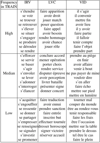
Frequency IRV LVC VID
in TRAIN
s’´etendre faire apparition il s’agir se voir avoir droit il convenir se trouver jouer match mettre fin se retrouver poser question avoir lieu s’´elever faire appel il y avoir High se situer avoir besoin faire partie
s’engager rendre hommage il falloir se produire avoir chance tenir compte se d´erouler jouer rˆole faire l’objet
se rendre prendre part
s’efforcer conclure accord prendre au pi`ege se servir mener op´eration en finir se baser porter choix avoir affaire
s’agir rendre service venir `a bout Median s’envoler disputer ´epreuve ne pas payer de mine
se lever avoir perception vouloir dire s’adonner livrer bataille s’en aller s’interroger pr´esenter signe faire ´echo
s’´elancer donner concert mettre sur pied mettre en lumi`ere s’acquitter faire traduction tourner mal s’engouffrer avoir ennui couper du monde
se ressentir prendre sanction ˆetre au rendez-vous Low se donner faire entr´ee tenir responsable
se partager inscrire but faire les frais s’empresser effectuer tourn´ee ˆetre l’occasion se renseignerdresser horoscope mettre sur la table
se signaler signer victoire prendre le dessus s’investir r´eserver accueil tel ˆetre le cas
se promener faire le plein
Table 8: Verbal multiword expression types (for IRV, LVC and VID categories) in WebSample (mentioned in Table 6). MVC entendre parler faire remarquer faire savoir laisser tomber
Table 9: Verbal multiword expression types (for MVC category) in WebSample (mentioned in Table 6).
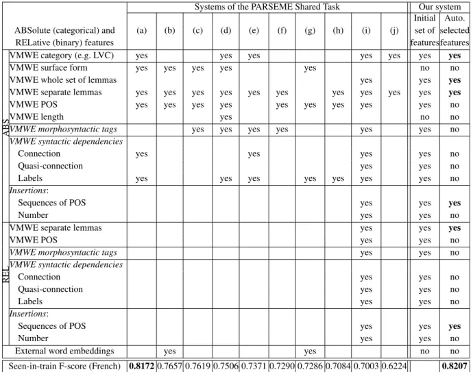
B Appendix: Features used for VMWE identification in the state-of-the-art works
Systems of the PARSEME Shared Task Our system Initial Auto. ABSolute (categorical) and (a) (b) (c) (d) (e) (f) (g) (h) (i) (j) set of selected
RELative (binary) features featuresfeatures
ABS
VMWE category (e.g. LVC) yes yes yes yes yes yes yes
VMWE surface form yes yes yes yes yes no no
VMWE whole set of lemmas yes yes yes
VMWE separate lemmas yes yes yes yes yes yes yes yes yes yes yes
VMWE POS yes yes yes yes yes yes yes yes yes no
VMWE length yes no no
VMWE morphosyntactic tags yes yes yes yes yes yes no
VMWE syntactic dependencies
Connection yes yes yes yes no
Quasi-connection yes yes no
Labels yes yes yes yes yes yes yes no
Insertions:
Sequences of POS yes yes yes
Number yes yes no
REL
VMWE separate lemmas yes yes yes
VMWE POS yes yes no
VMWE morphosyntactic tags yes yes no
VMWE syntactic dependencies
Connection yes yes no
Quasi-connection yes yes no
Labels yes yes no
Insertions:
Sequences of POS yes yes yes
Number yes yes no
External word embeddings yes yes no no
Seen-in-train F-score (French) 0.8172 0.7657 0.7619 0.7506 0.7371 0.7290 0.7286 0.7084 0.7003 0.6224 0.8207
Table 10: Relevant features for VMWE identification and performances for the previously seen VMWEs for our system vs. the systems in the PARSEME Shared Task (Ramisch et al.,2018): (a)Waszczuk(2018), (b)Taslimipoor and Rohanian(2018), (c)Boros and Burtica(2018), (d)Stodden et al.(2018), (e)Moreau et al.(2018) (CRF-DepTree-categs system), (f)Moreau et al.(2018) (CRF-Seq-nocategs system), (g)Berk et al.(2018), (h)Ehren et al.(2018), (i)Pasquer et al.(2018), (j)Zampieri et al.(2018)