Nonlinear dynamical properties of an oscillating tip-cantilever system in the tapping mode

HAL Id: hal-00011145

https://hal.archives-ouvertes.fr/hal-00011145

Submitted on 11 Oct 2005

HAL is a multi-disciplinary open access

archive for the deposit and dissemination of

sci-entific research documents, whether they are

pub-lished or not. The documents may come from

teaching and research institutions in France or

abroad, or from public or private research centers.

L’archive ouverte pluridisciplinaire HAL, est

destinée au dépôt et à la diffusion de documents

scientifiques de niveau recherche, publiés ou non,

émanant des établissements d’enseignement et de

recherche français ou étrangers, des laboratoires

publics ou privés.

Nonlinear dynamical properties of an oscillating

tip-cantilever system in the tapping mode

Laurent Nony, Rodolphe Boisgard, Jean-Pierre Aimé

To cite this version:

Laurent Nony, Rodolphe Boisgard, Jean-Pierre Aimé. Nonlinear dynamical properties of an oscillating

tip-cantilever system in the tapping mode. Journal of Chemical Physics, American Institute of Physics,

1999, 111(4), pp.1615-1627. �10.1063/1.479422�. �hal-00011145�

Nonlinear dynamical properties of an oscillating tip–cantilever system

in the tapping mode

L. Nony, R. Boisgard, and J. P. Aime´a)

CPMOH Universite´ Bordeaux I, 351 Cours de la Libe´ration, F-33405 Talence, France

PUBLISHED IN J. Chem. Phys. 111(4), 1615-1627 1999.~!

The dynamical properties of an oscillating tip–cantilever system are now widely used in the field of scanning force microscopy. The aim of the present work is to get analytical expressions describing the nonlinear dynamical properties of the oscillator in noncontact and intermittent contact situations in the tapping mode. Three situations are investigated: the pure attractive interaction, the pure repulsive interaction, and a mixing of the two. The analytical solutions obtained allow general trends to be extracted: the noncontact and the intermittent contact show a very discriminate variation of the phase. Therefore the measurement of the phase becomes a simple way to identify whether or not the tip touches the surface during the oscillating period. It is also found that the key parameter governing the structure of the dynamical properties is the product of the quality factor by a reduced stiffness. In the attractive regime, the reduced stiffness is the ratio of an attractive effective stiffness and the cantilever one. In the repulsive regime, the reduced stiffness is the ratio between the contact stiffness and the cantilever one. The quality factor plays an important role. For large values of the quality factor; it is predicted that a pure topography can be obtained whatever the value of the contact stiffness. For a smaller quality factor, the oscillator becomes more sensitive to change of the local mechanical properties. As a direct consequence, varying the quality factor, for example with a vacuum chamber, would be a very interesting way to investigate soft materials either to access topographic information or nanomechanical properties.

@~!#

I. INTRODUCTION

Recent developments in the field of scanning force mi-croscopy~SFM! are focused on the behavior of the dynami-cal properties of an oscillating tip–cantilever system ~OTCL!. Experimentally, the use of the OTCL to probe sur-face properties at the local scale, from the nanometer to a few picometers, is done with two different operating modes. One mode keeps the oscillating amplitude constant, and the measured quantities are shift in resonance frequency as a function of the tip–surface distance. In this case, recording image is obtained by moving up and down the surface in order to keep a chosen frequency shift constant. These ex-periments are performed without any contact between the tip and the sample; thus frequency shifts are a measure of the attractive force between the tip and the surface. Spectacular experimental results have shown that images giving a con-trast at a few ten picometers can be achieved.1–5Companion theoretical developments suggest that the high sensitivity of this mode is due to the nonlinear dynamical properties of the OTCL at the proximity of the surface.6–8Recent experimen-tal results show variations of the image as a function of the chosen frequency shift.4 Here again, it does appear that the images obtained depend of several factors, among them the OTCL properties and the fine structure of the tip. There re-mains a quite long way to completely understand the image obtained, a general and well-known problem in the field of the local probe method.

With the second mode, a drive frequency is chosen. The

feedback loop is used to maintain constant the amplitude of the OTCL. The recorded images are the vertical displace-ments needed to keep the amplitude constant and the corre-sponding phase of the OTCL. This mode, commonly called tapping, is often used in intermittent contact ~IC!, that is, during a part of the oscillating period the tip touches the surface but images can also be recorded without any contact. This mode had been conceived mainly to reduce the shear forces at the interface between the tip and the surface. So that a new area is open in which soft materials, polymers, and biological systems can be investigated without producing significant damages. Numerous experimental results have shown the ability of this mode to image soft materials.9–12 Among them, phase contrast inversion as a function of the set point and images of triblock copolymers are quite con-vincing of the great potentiality of this mode. But here again, recording a true topography is far to be achieved; more cor-rectly one may discuss in terms of nanomechanical proper-ties of the sample probed by this mode.12–16Several theoret-ical approaches have been dedicated to the tapping, part of them being numerical simulations.14,17–21 The major draw-back of numerical simulations is the difficulty to give general routes and simple predictions to understand and define ex-perimental strategies.

The present work is an attempt to extract analytical ex-pressions describing the tapping mode. As shown in preced-ing papers,7,19 the nonlinear dynamics of the OTCL in an attractive field is quite complicated and indeed do show a subtle different behavior depending of the mode chosen.7,14,20,22Even more complicated is the situation when

a!_{Electronic mail: jpaime@cribx1.u-bordeaux.fr}

1615

the tip is brought into contact to the sample. Therefore very simple hypotheses are used in order to extract analytical so-lutions giving the essential trends of the OTCL response.

The paper is organized as follows: the theoretical part is divided in two sections. The attractive regime is presented in Sec. II. The phase and amplitude variations as a function of the OTCL-surface distance are shown for a drive frequency slightly below the resonance frequency. In Sec. III, the IC case is first discussed with a simple repulsive harmonic po-tential, then an attractive interaction is added. Section IV is dedicated to a brief discussion and a few experimental results are given. In Appendix A and B are given a detailed techni-cal description of the theoretitechni-cal approach and of the experi-mental conditions, respectively.

II. ATTRACTIVE REGIME

In a tapping experiment, a tip–microlever system is kept vibrating at a drive frequencyvnear a surface. Recording of the phase and vertical displacements of the piezoelectric ce-ramic holding the sample are made thanks to a feedback loop keeping the amplitude constant. To understand the origin of the image contrast, one must understand changes of the am-plitude and phase, A(D) and w(D), respectively, as func-tions of the OTCL-surface distance D. Recording A(D) and

w(D) is achieved by making approach–retract curves. The scan is stopped at a given location (X;Y ) in the horizontal plane of the sample, then a periodic motion along the vertical Z-axis is performed. In these experiments, series of approach–retract curves are obtained providing information on the properties of the dynamical behavior of the OTCL as a function of D and properties of the sample at the local scale. The ultimate goal is to extract the sample properties from variations of A(D) andw(D).

The attractive interaction between the tip and the sample is assumed to be a sphere–plane interaction involving the disperse part of the van der Waals interaction@see Eq. ~5!#. For distances from the surface above a few nanometers, the attractive force is negligible and a forced, damped oscillator satisfactorily describes the OTCL. The differential equation describing the harmonic behavior, i.e., amplitude and phase relationships with the frequency, is given by:

x¨~t!1v0

Q x˙~t!1v0 2

x~t!5 f

mcos~vt!, ~1!

with, respectively, v0, Q, and m the resonance frequency,

quality factor, and effective mass of the OTCL. f andvare the external drive force and drive frequency.

The stationary solution is:

x~t!5A_free~v!cos@vt1w_free~v!#, ~2! where Afree(v), andwfree(v) are the amplitude and phase of

the oscillations at the drive frequency. Since the oscillator responds with delay to the excitation, the sign of the phase chosen in Eq. ~2! means that wfree(v) varies in the domain

@2180°; 0°#. With reduced coordinates: u5v/v0 and

afree(u)5Afree(u)/A0, with A0 the amplitude at the

reso-nance frequency (u51) given by:

A05 f m Q v0 2, ~3!

the solutions of Eq. ~1! are:

afree~u!5

1

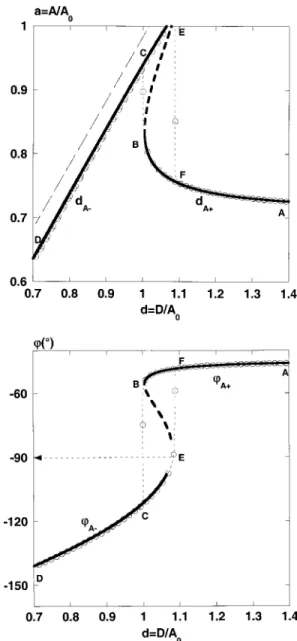
A

FIG. 1. ~a! Variations of the amplitude as a function of the OTCL-surface distance in a pure attractive field corresponding to an approach–retract curve. Numerical simulation~empty circles! and calculated with Eq. ~7a!

~thick continuous line!. The unstable part of the analytical branch dA1~point B to E! is represented with a thick dotted line. The parameters used are

A0510 nm, Q550, u50.990 05, kc54.935 N m21, H58.1675310219J, R520 nm. The corresponding value of ka is ka53.3131023(Qka

50.1655). The free amplitude is afree51/&50.707. The equation d5a

~thin dashed line! gives the location of the surface. The bistable structure is

shown with the cycle BCEF.~b! Variations of the phase associated to the variation of the amplitude given in Fig. 1~a! @Eq. ~7b!#. The phase jump leads to a noncontact phase below290°. The analytical brancheswA1and

wA2don’t join exactly. This is uniquely due to the numerical sampling used

wfree~u!5arctan

S

u

Q~u221!

D

During an approach–retract curve, the oscillator experi-ences both a pure attractive and an attractive–repulsive field. A van der Waals attractive field leads to a nonlinear dynamic behavior of the OTCL and can generate a hysteresis cycle in the approach–retract curve.16–19 An approach based on a variational principle had shown that analytical expressions could be derived describing the nonlinear behavior of the OTCL.19

The aim of parts II and III is to develop the analytical model with a more precise description of the noncontact ~NC! and IC situations including phase variations during an

approach–retract curve. In Appendix A, detailed calculations are given. The main results are presented below.

In this part, we assume that the OTCL never touches the surface and is described as a forced damped oscillator plus an interacting van der Waals disperse term with a sphere– plane geometry.23 The dissipation function added to the La-grangian is W5xFd, where Fd52(mv0/Q)xI˙ is calculated

along the physical path, thus is not a varied parameter.24

L5T2U1W ~5! L51 2mx˙ 2_~t!2

F

G

where H is the Hamaker constant, R the tip’s apex radius and D the distance between the surface of the sample and the equilibrium position at rest of the OTCL. We focus on the stationary harmonic state, thus the trial function used has the stationary harmonic form of Eq.~2!. With the reduced coor-dinate d5D/A0, the analytical approach leads to the two

coupled equations: cos~w!5Qa~12u2!2 aQk_a 3~d22a2!3/2 ~6! sin~w!52ua, where ka5HR/kcA0 3

is a dimensionless parameter. Since kc5mv0

2

is the cantilever stiffness, HR/A₀3 has the dimen-sion of a stiffness and can be related to a strength of the attractive interaction. Therefore varying ka with A0 is

equivalent to change the strength of the attractive interaction: for example, a large~small! A0corresponds to a small~large!

ka. The solutions of Eqs.~6! are:

d_A65

A

S

S

A

D

D

S

D

Note that setting ka50 in Eq. ~7b!, i.e., no attractive

inter-action, leads to the phase equation of the harmonic oscillator @Eq. ~4!#. As a consequence of the nonlinear behavior, at a given distance d, the amplitude and phase of the OTCL de-pends on the drive amplitude through the cubic term A₀3.

Equations~7a! and ~7b! give two physical branches for the amplitude and the phase ~see Appendix A!. For drive frequencies slightly below the resonance one amplitude and phase exhibit a hysteresis cycle that disappears as the mag-nitude of Qka increases@see Figs. 1~a!, 1~b!, and 2~a!, 2~b!#.

In Figs. 1 and 2 are reported amplitude and phase varia-tions calculated from Eqs.~7a! and ~7b! and the

correspond-FIG. 2.~a! Variation of the amplitude similar to the one shown in Fig. 1~a! but with the parameters: A056 nm, Q550, u50.990 05, kc50.247 N m21, H510219J, R520 nm, corresponding to a larger value ofka,ka53.752

31022_(Qk

a51.876). The unstable behavior and the hysteresis cycle have disappeared. ~b! Variation of the phase associated to the variation of the amplitude shown in Fig. 2~a! @Eq. ~7b!#. The phase jump disappears and the phase crosses continuously the290° value, the noncontact phase is below

ing numerical results. The numerical simulation solves the following differential equation based on Eq.~1! plus the in-teracting term, x¨(t)1(v0/Q)x(t)1v0

2

x(t)5( f /m)cos(vt)

2HR/6m(D2x(t))2_{, with a Runge–Kutta 4 method from}

arbitrary initial conditions. We assume that the oscillator is in its harmonic state for each step of the implementation. This is validated by an adiabatic criterion, which evaluates the number of points for the whole calculus for a given value of the quality factor. Amplitude and phase variations are then calculated thanks to a numerical synchronic detection filter-ing the first harmonic, n51. To verify that the use of the harmonic solution was efficient to describe the nonlinear be-havior, thus validate the analytical model, several numerical simulations were done with a synchronic detection filtering the second harmonic, n52. We found that the amplitude variations were less than 0.3% of the ones for n51. For the smaller Qk_avalue@Figs. 1~a!, 1~b!#, letters illustrate the hys-teresis cycle and the bistable behavior of the OTCL. When bifurcation occurs during the approach~retract!, point B ~E!, the numerical solution jumps to its stable upper ~lower! branch in amplitude, point C ~F!, instead of following the unstable branch BE.

Then, since d decreases, the strength of the attractive field increases, from which an increase of the amplitude is expected. The reduction of the amplitude predicted, and observed,16,19is a nonintuitive result~C to D!. The reduction of the amplitude is due to change of the phase relationship between the OTCL and the excitation, the phase getting a value below290° @Fig. 1~b! from C to D#. Thus, the attrac-tive interaction acts as a repulsive one, leading to a decrease of the amplitude.19

The whole variation of the phase, phase jump, and cycle of hysteresis @Fig. 1~b!#, is similar to the one of the ampli-tude@Fig. 1~a!#. For a small value of Qk_a, the phase jumps below290° and an hysteresis cycle follows. For a large Qka

value @Figs. 2~a!, 2~b!#, the phase crosses the value of 290° continuously and the approach and retract curves are identi-cal. Measurement of the phase is very useful to identify NC situations. As discussed below, as soon as the phase is less than290°, the attractive regime is dominant.

At this stage, it is worth discussing in more detail the physical origin of the variation of the phase. Within the lin-ear response theory, the instantaneous dissipated power is a function of the phase value through a sin function. When a nonlinear dynamical behavior occurs, the variation of the phase is not uniquely related to the dissipation but also to the distortion of the resonance peak.

As shown with the introduction of the dimensionless pa-rameterka @Eqs. ~7!#, contrary to a linear behavior, the

forc-ing term cannot be scaled out. The magnitude of the drive amplitude becomes a new operative parameter as much as the strength of the nonlinear coupling term. At fixed drive frequency and fixed drive amplitude, when the OTCL ap-proaches the surface, the oscillating amplitude and the strength of the nonlinear coupling term vary. As a conse-quence, a phase variation is expected without involving a particular change of the dissipating process. In the present case, uniquely the attractive field is involved. From Eqs.~7! we derived the equation giving the shape of the resonance peak as a function of the OTCL-surface distance, d:

u5

A

F

S

A

S

D

DG

Here we focus on the variations of the phase when a drive frequency is slightly below the resonance one. The case of a drive frequency at the resonance one or above gives a simpler structure and can be straightforwardly deduced. In Figs. 3~a! and 3~b! are given the evolutions of the resonance peak as a function of d and the corresponding phase varia-tions when the OTCL moves towards the surface. At dis-tances d large enough, say a few nanometers, the peak keeps its resonance shape and the phase remains roughly constant @domain ~a!#. When the peak starts to distort and the location of u crosses the bifurcation point, the phase jumps to the lower branch @domain ~b!#. At a closer distance, the peak further distorts and the phase goes towards the2180° value @domain ~c!#. Therefore, the phase variation provides a pre-cise information about the stationary state of the OTCL. This statement is particularly verified when IC situations take place.

III. INTERMITTENT CONTACT_„IC_…REGIME

A. Pure repulsive field

The IC situation is given by a.d. In a first step, the attractive interaction is considered as being negligible (H 50). The repulsive field acts during a short part of the OTCL period, typically a hundredth of the period. Thus the action is defined between the two instants t_i50 and t_f 5@arccos(D/A)#/v. In order to get an analytical expression, the repulsive interaction is assumed to have a simple har-monic form: (1/2)ks(x(t)2D)2, where ks is the contact

stiffness scaling as k_s5G_sf, with f the diameter of the contact area involved in the IC situations and Gs the

Young’s modulus of the sample.25,26For small indentations, (a2d)/a!1, the variational principle gives the couple of

cos~w!5Qa~12u2!14& 3p Qksa

S

D

where ks5ks/kc is the ratio between the contact stiffness

and the cantilever stiffness. Solving Eq. ~9! gives:

dR5a

H

S

A

D

J

S

S

D

D

There is one physical branch of solutions in amplitude and in phase ~see Appendix A!. The key parameter is now Qks in

place of Qka.

The slope of the variation of the amplitude with d,s(a)

5da/dd, of an approach–retract curve is a fundamental

pa-rameter. Firstly, the slope contains information about the na-nomechanical properties of the sample. Secondly, the slope at a given setpoint, that is at a given amplitude reduction at which an image is recorded, controls the vertical displace-ment of the piezoelectric actuator. Equation~10a! predicts a slope function of the Qks parameter. As a consequence, Eq.

~10a! predicts that even for soft materials, a large Q value could give a true topography of the surface, s(a)51, without any access to the mechanical properties of the sample. To be more quantitative, an analytical expression of the slope can be derived from Eq. ~10a!:

s~a!5

1 11 b~a!

~Qks!2/3

, ~11!

where b(a) is a complex expression of a, and a_free. The maximum value ofb(a) is around 5 and is reached for value of the amplitude close to afree. Therefore for Qks@10, the

slope is 1 over the whole domain of variation of the ampli-tude. Practically, one can evaluate the Young’s modulus Gs

above which the slope is 1 whatever the value of the reduced amplitude a. In air, the quality factor is around 300. Choos-ing kc510 N m21, we get ks@0.33 N m21 and with f

51 nm, Gs@3.33108N m22.

FIG. 4. Influence of the quality factor Q on the slope in the IC case with uniquely a repulsive field@Eq. ~11!#. The slopes as a function of the reduced stiffness ks are calculated at the reduced amplitude a50.65. The other parameters are, u50.9900, afree50.707, and kc510 N m21.

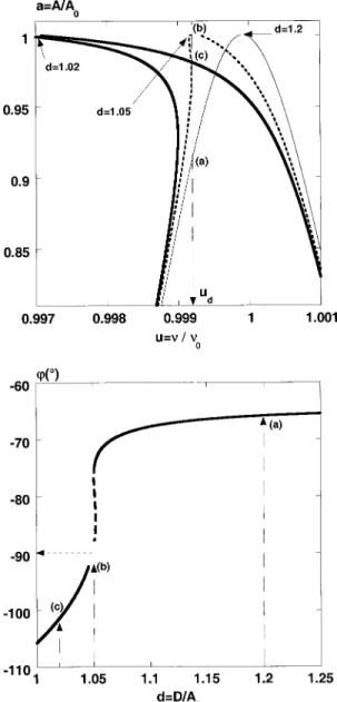
FIG. 3. ~a! Distortion of the resonance peak under the action of the attrac-tive field for three values of the distance d@Eq. ~8!#. The parameters are

A0515 nm, Q5300, and ka51.4831024. Letters indicate the transition between the stable behavior~domain ~a!, d51.2) with the free amplitude associated to ud50.9992, afree50.91, to the bistable behavior leading to an

increase of the amplitude~domain ~b!, d51.05) and then the reduction of the amplitude~domain ~c!, d51.02). For clarity, only the upper part of the resonance peak is shown.~b! Analytical approach–retract curve of the phase illustrating the distortion of the resonance peak shown in Fig. 3~a!. Arrows indicate the different points shown in Fig. 3~a! at ud50.9992.

Equation~11! predicts a nonlinear variation of the slope, but, within a selected range of amplitudes a ~see Sec. IV, Table I!, a k_s2/3 dependence is extracted that differs signifi-cantly from the one calculated for the static deflection mode. With the static mode, the slope, ssd, measured with a force

curve is given by:27

ssd5 1 11kc ks 5 1 11 1 ks , ~12!

besides a power law, the quality factor Q plays a major role. To illustrate the influence of the quality factor, the variations of the slope as a function ofksfor Q550, 500, and 5000 are

reported in Fig. 4.

A comparison with a numerical simulation@the numeri-cal simulation describing the intermittent contact is solved with the same procedure as the previous one, but the non-contact equation is replaced by a non-contact equation of the form, x¨(t)1(v0/Q)x(t)1v0

2

x(t)5( f /m)cos(vt)1(ks/m)

3(x(t)2D)] of the predicted variations of the amplitude and of the phase is given in Figs. 5~a! and 5~b!. The numerical results validate the small indentation approximation. With

ks50.0239 and Q550 a slope of about 0.22 is calculated

whereas with Q55000 and the sameks, the slope is 0.93.

The phase wR is above 290° during the entire

approach–retract curve. When the oscillator touches the sur-face, the phase increases from its free value to 0°. This result emphasizes the difference between the NC state ~phase be-low 290°! and the IC state ~phase above 290°!.

B. Attractive and repulsive fields

A more realistic description of the IC includes an attrac-tive interaction. To do so, we assume that the tip experiences

the repulsive field during the two instants @ti;tf#, and an

attractive van der Waals field during the time of the oscilla-tion @tf;T52p/v#.

Unfortunately, because of the diverging behavior of the attractive field at d5a, it is difficult to obtain a simple, tractable, analytical solution. To get an analytical solution, we first assume that the attractive field acts during the whole period T,tf being a small part of the period. Then, the

attrac-tive contribution is evaluated for d5a1d˜_c, i.e., at the clos-est NC distance from the surface, where d˜c is the reduced

coordinate of the contact distance dc50.165 nm:23 d˜c

5dc/A0. With these conditions, we get:

cos~w!5Qa~12u2!14&

3p Qksa

S

D

A

Solving Eq. ~13! gives a cubic equation from which d 5 f (a) is easily extracted.

aX3_2C50⇔X5

S

a

D

1/3

, ~14!

with C5(3p/4&)@Qa(u221)1

A

6&d˜_c3/2)(1/

A

A

H

S

D

J

S

S

D

D

Here again, a unique physical branch of solution is given by Eqs. ~15! ~see Appendix A!. As for the pure repulsive case, Eq. ~15a! predicts a (Qks)2/3 dependence, but the relative

importance of this parameter now becomes dependent of the magnitude of (Qks). While for small amplitudes~largeka)

the slope is a complex function of k_a and k_s, for large amplitudes~small ka), the OTCL becomes mostly sensitive

to a pure repulsive field. Therefore, at large amplitudes, we expect the experimental curves to be suitably described with Eqs. ~10!.

A typical IC approach–retract curve requires to combine the solutions given by Eqs. ~15! with the analytical results obtained with uniquely a pure attractive field @Eqs. ~7a! and ~7b!#. Theoretically, the equation of the surface is d5a, while a more realistic description preventing the diverging

behavior uses d5a1d˜_c. A direct consequence is that branches of solution dA1(dA2) obtained with a pure

attrac-tive field might in fact touch the surface.

For smallks ~large A0), at the bifurcation spot@point B,

Figs. 6~a! and 6~b!# the branch of solution dA2(wA2) is

above the surface d5a1d˜c, meaning that the tip jumps

to-wards the upper IC branch dAR(wAR). ~point C!. Then, the

amplitude ~phase! decreases ~increases! ~D!. When the sur-face is retracted, the oscillator follows back the branch dAR(wAR) until it reaches the maximum value of the

ampli-tude ~phase!, which is solution of the equation dAR5dA1

(wAR5wA1)~point E! ~or equivalently dAR5a1d˜c). At this

point, as it is usually observed experimentally, the value of the amplitude is larger than the free one but smaller than thee

resonance one for which a51. At the same time, the value of the phase is smaller than the free one but larger than the resonance one (w5290°). The structure of the whole curve exhibits a hysteresis cycle. At the end of the retract, the

amplitude~phase! jumps back to its free value ~F!.

At intermediateka values, more complex situations can

be found that lead to a mixing of NC and IC situations. Figures 7~a! and 7~b! display most of the situations pre-dicted. Since the bifurcation of the phase unambiguously dis-criminate between NC and IC stationary states, phase varia-tions are uniquely reported.

For values of ka not too large, the approach–retract

curve presents the structure of Fig. 6~b! @Fig. 7~a!: from A1

FIG. 5. ~a! Evaluation of the small indentations approximation leading to Eqs. ~10!. The common parameters are A0520 nm, kc53.55 N m21, H

50 J, R55 nm. The location of the surface is given by the thick

dashed-dotted line. Numerical results and curves calculated with Eq.~10a! have been performed with three different sets of parameters:~i! the analytical curve~thick continuous line! and the numerical simulation ~empty squares! were computed with Q550, u50.990 05, and ks50.085 N m21(ks

50.0239 and Qks51.195). The average slope extracted with a linear fit is s150.22. Even for a small reduced stiffnessks, the comparison between the numerical results and the analytical one gives a good agreement down to the reduced amplitude a50.4. ~ii! The analytical curve ~thin continuous line! and the numerical simulation ~empty circles! were obtained with Q

550, u50.990 05, and ks50.85 N m21(ks50.239 Qks511.95). ~iii! The third set of parameters is Q55000, u50.999 90, and ks50.085 N m21(ks

50.0239 Qks5119.5), analytical curve ~thin dotted line! and numerical simulation~empty triangles!. For these two sets of parameter, similar results are obtained on the whole range of variation of the reduced amplitude with a slope s25s350.93. ~b! Comparison of the variations of the phase between

the numerical simulations and the analytical curves calculated with Eq.

~10b!. The parameters are the same as the ones used for Fig. 5~a!. The IC

phases are above290°.

FIG. 6. ~a! An analytical approach–retract curve showing the variation of the amplitude~thick continuous line!. The attractive interaction is incorpo-rated to describe the IC regime. The thick dashed lines give the unphysical branches. The branches dA6are calculated with Eq.~7a! with A0510 nm,

Q550, u50.9900, andka51024. The branch dARis calculated with Eq.

~15a! with the additional reduced stiffness ks50.02. The path BCEF de-scribes the cycle of hysteresis. The thin dashed-dotted line gives the location of the surface.~b! Analytical approach–retract curve showing the variation of the phase associated to the variation of the amplitude shown in Fig. 6~a!. wARis above290° over the whole approach and the whole retract of the surface.

to F₁]. At a larger value ofk_a, the branches w_A1 andw_AR join exactly atw5290° @Fig. 7~a!: from A₂to F₂]. This is still a situation of IC.

Whenkais further increased, again during the approach

the OTCL jumps down to the wAR branch of solutions@Fig.

7~b!, points A3to C3], while during the retract wAR doesn’t

join wA₁ anymore. During the retract, the phase associated

to the wAR branch reaches the value of the resonance one:

290° (E3), then jumps down to thewA2 branch (F3) before

reaching thewA1branch (H3). This situation gives a second

bistable behavior of the oscillator with an intermediate NC situation.

For large values of k_a, the branch of solutions w_AR is too far to be reached during the approach @Fig. 7~b!, point B₄]. The stable branch is uniquely the NC one and the OTCL follows the usual NC path @Fig. 7~b!, points C₄ to A₄].

IV. DISCUSSION

Because of the nonlinear behavior of the OTCL and of the mixing of IC and NC stationary states, complex situa-tions can happen as those shown in Fig. 7~b!. But, while some of them will not be easy to observe experimentally, others, theoretically forbidden, will occur because of tip~or surface! pollution. In the present part are given some typical results, showing that the observed variations of the phase allow the IC and NC situations to be easily discriminated. Also some unpredicted situations are presented. Finally, we briefly discuss two points that have not been analytically solved. One is the case of dissipating samples, a rather im-portant point for soft materials, the second concerns numeri-cal results in which are included the Hertz model to describe the IC state.

The experimental results shown in Figs. 8 and 9 were performed in a glove box on silica surfaces and polystyrene polymer films of molecular weight MW5200 000. The silica

surfaces were prepared as described in Ref. 28. Both silica and polymer surfaces can be considered as hard surfaces, the polymer film for high molecular weights being mechanically inert under the action of the oscillating tip in the attractive regime.16In the glove box, the p.p.m. of water is achieved so that capillary forces are negligible ~see also Appendix B!.

FIG. 7. ~a! Analytical approach–retract curves showing the variations of the phase for two values of the drive amplitude @Eqs. ~7b! and ~15b!#. A0

520 nm ~thick lines! and A057 nm ~thin lines!. Dashed lines represent the

unstable branches and branches which cannot be reached. The parameters are Q5400, u50.9986,ks50.1, and ka53.531026, and 8.1631025 for A0520 nm and A057 nm, respectively. The path BiCiEiFi describes the cycle of hysteresis. For this two-set of parameters, the branchwA @Eq. ~7b!# is never reached.~b! Same as in Fig. 7~a! but with two others values of A0.

A056 nm ~thick lines! illustrates a second unstable behavior ~points E3to

F3) and A053 nm ~thin lines! illustrates a pure NC situation ~branchwA) for which the IC is never reached. The parameterskaare equal toka51.3

31024_{and 1.04310}23_{for A}

056 nm and A053 nm, respectively.

FIG. 8. Experimental approach–retract curves showing the variation of the phase on a polystyrene polymer film of molecular weight Mw5200 000. The experimental drive amplitudes give A0555, 44, 30, and 20 nm. The

OTCL used is the OTCL1~Appendix B!. The zero of the vertical location of the surface is set arbitrarily ~see Appendix B!. The NC stationary state occurs at a value as high as Afree50.7073A0, with A0530 nm, thus

The general trend predicted by Eqs. ~15! is in good agreement with the one measured. The relative importance of the dimensionless parameter Qkacan be checked by varying

the drive amplitude,19thus A0, or using a large tip radius~or

a crashed tip!, a larger HR product. With a crashed tip, a pure attractive regime shown by the variation of the phase occurs at a A0 value as high as 30 nm ~Fig. 8!. For NC

stationary states exhibiting a bifurcation, as soon as the OTCL had crossed the bifurcation point, the phase varies slowly and its variation is practically independent of the A0

value, thus a similar variation is observed with A0520 nm.

With a second OTCL, the pure attractive regime uniquely occurs for small values of A₀ ~below A₀54 nm,) from which is deduced that the tip is much smaller~Fig. 9!. For such a small tip radius, a bifurcation structure is more difficult to observe and the phase crosses almost continu-ously the290° value @as shown theoretically, Fig. 2~b!#.

The situations showing a jump from an IC branch to a NC one during the retraction of the surface@path E3F3G3H3,

Fig. 7~b!# were not experimentally encountered. The reason is probably that this type of jump occurs at a spot close to the one corresponding to the usual instability jumping back to the free values of the phase and amplitude. Nevertheless, bifurcation structures resembling those can be found for soft

FIG. 9. Experimental approach–retract curves performed with the OTCL2 on a silica surface. The experimental conditions are given in Appendix B. At

A059 nm, Afree56.4 nm, the OTCL remains in a well-defined IC stationary

state. The NC state is observed for values equal or below A054 nm (Afree

52.8 nm). For such a low value of the amplitude, the instability has

disap-peared and the variation of the phase resembles the theoretical one given in Fig. 2~b!.

FIG. 10. Variation of the amplitude and the phase observed on a mica surface with the OTCL3 with A0541 nm. Phase and amplitude indicate an

IC state.

FIG. 11. Variation of the amplitude and the phase observed on a mica surface with the OTCL3 with A0532 nm. The NC branch is the stable one

@see the fourth case in Fig. 7~b!#, but an instability occurs ~point F! and the

IC branch is reached~point I!. Such a jump is not predicted. Here is in-volved a possible pollution of the tip and/or of the surface~see text!.

FIG. 12. Variation of the amplitude as a function of the OTCL-surface distance calculated with Eq.~15a!. The parameters are the ones used in the Table. The dotted curve corresponds to the pure attractive case@Eq. ~7a!#. The continuous lines from the right to the left have been calculated with the Young Modulus 100, 10, 1, and 0.1 GPa, respectively. The arrows indicate the domain of variation used to fit the curve with a linear function~see Table!.

materials. In that case, the bifurcation is due to the growth of a viscoelastic nanoprotuberance under the action of the at-tractive field of the OTCL.16

It’s far beyond the scope of the present work to discuss in detail such a behavior. Moreover, the study of polymer films made of tribloc that exhibit a regular structure at the mesoscopic scale with different mechanical responses10,11,12 is more suitable. As a matter of fact such a material, and in general the mixing of hard and soft materials, exhibit a wide variety of situations that requires a specific analysis.14,15

The latter example concerns the study of a mica surface in the glove box with a rather large tip~Figs. 10 and 11!. The structure observed is reminiscent of the fourth case given in Fig. 7~b! ~path B4C4E4F4). At a very large drive amplitude,

A0541 nm, the usual variations of the IC state are observed

~Fig. 10!. At a slightly lower one, A0532 nm, the OTCL

follows the NC branch then suddenly jumps to the IC branch to reach the value w5290°. During the retract, the OTCL follows the IC branch untilw5290° is reached, then jumps down to the NC branch~Fig. 11!. This situation corresponds to the fourth case for which the NC branch is the stable one and the IC state should normally not be reached@Fig. 7~b!#. In other words, experimental results similar to the ones shown in Fig. 8 (A₀530 and 20 nm!, where uniquely the NC branch is available, should be observed.

To explain the observed IC state, the most reasonable hypothesis is the occurrence of pollution either on the tip or on the surface that allows an IC situation to happen quench-ing the OTCL in the IC state. This can be explained with the fact that the average attractive field between the OTCL and the surface varies as 1/

A

Not included in the above analysis is the influence of an additional dissipation when an IC state takes place. As stated above, great care must be taken to discuss phase variation as the result of a dissipating process. In any case, the introduc-tion of an addiintroduc-tional dissipaintroduc-tion will make almost impossible the search for an analytical solution without the use of as-sumptions making the whole attempt questionable. Numeri-cal simulations can help to identify the role of dissipation. Qualitatively some information can be used12,13,14but even in that case, the phenomenological approach does not give a clear meaning of what is really occurring. The additional

dissipation can be issue of the bulk viscoelastic properties of the sample, requiring that the volume involved is at least of the cubic micrometer.29Such a huge volume is certainly not involved in IC situations. If the dissipate process occurs at the interface between the tip and the surface, there is no simple analytical solutions and the description of the dissi-pating process remains quite complicated even in the case of the static deflection mode.27

Finally, a question arises about the validity of the simple harmonic model employed to describe the repulsive field. A somewhat more complicated approach is to introduce the Hertz model, which gives a nonlinear dependence between the indentation depth and the elastic force.25 The Hertz model describes an elastic contact between the tip and the sample and provides an evaluation of the contact stiffness as a function of the indentation depth. The introduction of the Hertz model doesn’t lead to a simple analytical solution.14 The results presented above are preserved, structure of the bifurcation, discrimination between the IC and NC states, and the main difference concerns the slope dependence as a function of the contact stiffness. The exponents found are slightly above the ones obtained with the harmonic approxi-mation~Table I and Fig. 12!.

Note that for reasonable values of k_a, numerical and analytical results give a power law close to 2/3. A simple analysis of Eq.~15a! indicates that with large amplitudes, the influence of the attractive field is reduced ask_a goes asymp-totically to zero, thus allowing the slope to have a simplest form as the one given in Eq. ~11!. Therefore, with a high amplitude it becomes easier to access the local mechanical properties more quantitatively. The other point is the impor-tant role of the quality factor Q. As shown with Eq.~11! and Eq.~15a!, the higher the quality factor, the larger the product Qks. Therefore to be very sensitive with an OTCL to access

at the nanomechanical properties of the sample requires a low Q factor, while to access the topographic structure re-quires a high Q factor and a high amplitude. The unique way to check the validity of these equations is to use a vacuum chamber in which the magnitude of the quality factor can be varied.

V. CONCLUSION

The aim of the present work was to extract analytical expressions describing the nonlinear behavior of an OTCL in

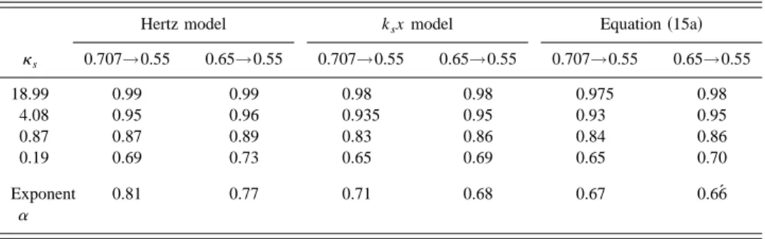
TABLE I. Comparison between the results obtained with two numerical simulations and the curve calculated with Eq.~15a!. Variations of the IC slope as a function of ks. Two domains of variations of the reduced amplitude a are chosen to be fitted with a linear approximation~from the free amplitude 0.707 to 0.55 and from 0.65 to 0.55!. The function used to extract the exponentais s51/(11C/ksa).

ks

Hertz model ksx model Equation~15a!

0.707→0.55 0.65→0.55 0.707→0.55 0.65→0.55 0.707→0.55 0.65→0.55 18.99 0.99 0.99 0.98 0.98 0.975 0.98 4.08 0.95 0.96 0.935 0.95 0.93 0.95 0.87 0.87 0.89 0.83 0.86 0.84 0.86 0.19 0.69 0.73 0.65 0.69 0.65 0.70 Exponent a 0.81 0.77 0.71 0.68 0.67 0.66´

the tapping mode. Three situations are considered: the pure attractive interaction, the pure repulsive interaction, and a mixing of the two. The analytical solutions give the variation of the amplitude and of the phase as a function of the OTCL-surface distance. The general evolutions predicted are in good agreement with the observed ones. The NC and IC stationary states can be discriminated by recording the varia-tion of the phase. The bifurcavaria-tion from a monostable to a bistable state is identified in the pure attractive regime. In the intermediate regime, because of the nonlinear behavior of the OTCL and the mixing of IC and NC stationary states, the structures of the bifurcation are more complex. Experimen-tally, it is easy to discriminate between the different situa-tions by varying the magnitude of the drive amplitude. The contribution of the attractive force can be significantly re-duced through the increase of the drive amplitude leading to an almost pure repulsive case, while a NC stationary state becomes dominant at small drive amplitudes. The quality factor Q is shown to be a key parameter. For large values of Q and large amplitudes a true topography is expected, while with a smaller value of Q, the OTCL becomes more sensitive to the local mechanical properties of the surface. Therefore, it does appear interesting to perform experiments on soft materials in a vacuum chamber in order to vary the quality factor.

APPENDIX A: THE VARIATIONAL PRINCIPLE 1. Pure attractive field

The principle of least action specifies that the action S@x(t)# being a functional of the path x(t) between two instants is extremal.

d$S@x~t!#%5d

H

E

t_i t_r

L~x;x;t!dt

J

where L is the Lagrangian of the system. The aim of the use of a variational principle is to employ a trial function x(t) allowing us to perform an analytical treatment. According to the fact that the oscillator essentially exhibits a harmonic behavior, the trial function used has the harmonic stationary form of Eq. ~2!, and therefore the action is defined on one oscillating period. The Lagrangian of the OTCL is defined as: L5T2U1W 51₂mx˙2~t!2

F

G

x~t!5A cos@vt1w#. ~A3!

The parameters of the path are A andw, and the principle of least action dS50 gives a set of two partial differential equations:

dS

dA50,

dS

dw50. ~A4!

Three terms are dissociated for the calculations of the action: S5S01Sint1Sdissip, ~A5!

where S0, Sint, and Sdissipare, respectively, the action of the

harmonic oscillator without dissipation, the action of the in-teracting term, and the action of the dissipating term.

S₀5

E

F

G

E

F

G

E

F

G

The calculation of S0 gives:

S05 pm 2vA 2_~v2_2v 0 2_!1pf v A cos~w!. ~A7!

x˙(t)52AIvsin(vt1w) is calculated along the physical

path,21 with AI andwI being fixed for the minimization. The integration gives:

Sdissip52

pmv0

Q AAI sin~w2wI !. ~A8!

The calculation of Sintrequires a more tedious, but

straight-forward, calculation:

Sint5

pHR

3vD

A

with e5A/D5a/d,1. Adding the expressions ~A7!, ~A8!, and~A9! gives the complete action:

S5pm 2vA 2_~v2_2v 0 2_!1pf v A cos~w!1 pHR 3v

A

]S ]A5 pm v A~v22v0 2_!1pf v cos~w!1 pHRA 3v~D2_2A2_!3/2 2pmv0 Q AI sin~w2wI !, ~A11!

whereas the minimization with respect towgives:

]S ]w52 pf v AI sin~w!2 pmv₀ Q AAI cos~w2wI !. ~A12! Since the underlined variables are calculated along the physi-cal path, A5AI and w5wI . With these conditions, solving

]S/]A50 and]S/]w50 and with the external drive force written as f5mv₀2A0/Q, ~A11! and ~A12! finally give the

cos~w!5Qa~12u2!2

aQk_a 3~d22a2!3/2

~A13! sin~w!52ua.

To get Eq. ~7!, the system is solved using the trigonometric relationship: cos(w)56

A

2. Pure repulsive field

The interacting term is given by:

Sint523

ks

2

E

arccos~D/A!/v

~x~t!2D!2_{dt. ~A14!}

Calculating the action, then using a Taylor’s expansion of arccos(D/A) for A'D, the calculations finally lead to Eq. ~9!:

cos~w!5Qa~12u2!14&

3p Qksa

S

D

With cos(w)56

A

two branches of variations. The fractional power law 2/3 in Eq. ~10a! implies to choose cos(w)51

A

3. Both attractive and repulsive fields The interacting term is given by:

Sint523

H

E

E

J

The attractive NC part is evaluated using the expression ~A9!. Then, a Taylor’s expansion of arccos(D/A) for A'D is used, and a physical surface given by d5a1d˜_cis introduced ~see text!. The calculations finally lead to the couple of equa-tions:

cos~w!5Qa~12u2!14&

3p Qksa

S

D

A

Here again, because of the fractional power law, only one physical branch of solution is available.

APPENDIX B: EXPERIMENTAL CONDITIONS

The experimental approach–retract curves were mea-sured with the tapping mode of a Nanoscope III from Digital

Instruments ~Santa Barbara, CA!. The cantilevers ~Nano-probe! have a typical resonance frequency around 300 kHz and a quality factor between 250 and 550~see Table B1!.

Two piezoactuators are needed to perform experiments with the tapping mode: one allowing the microlever to vi-brate at a given drive frequency with a given drive ampli-tude, and a second piezo to move the sample. During an approach–retract curve, the second piezo displaces the sample along the Z-axis while the other keeps constant the drive frequency and the drive amplitude.

1. Technical remarks: preparation of the experiment The resonance frequency and the quality factor are ex-tracted from measurements of the resonance peak~Cantilever Tune mode on the NIII!. Recording of the resonance peaks are made at distances from the surface between 500 nm and 1 mm. For distances above 10mm, it has been shown that parameters of the OTCL vary.12,30Change of the resonance amplitude and frequency had been attributed to the decrease of the thickness of a layer of air between the OTCL and the surface. The OTCL properties become stable as soon as the distance between the OTCL and the surface is around or smaller than one micrometer.

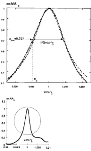
The quality factor Q is measured at A5A0/& ~at a

51/&50.707 with the reduced coordinates!. For large val-ues of Q, the quality factor is given by Q5n0/Dn, withDn

the frequency width at this amplitude. Using the reduced coordinates, a resonance curve is presented in Fig. B1 with the corresponding fit@Eq. ~4a!#. In many cases the resonance curves may exhibit an asymmetric shape and several bumps in the curve tails. Practically, the undesirable bumps can be resumed by clearing the lodgment of the cantilever and mov-ing the cantilever inside its lodgment.

At the very beginning, the resonance peak is often asymmet-ric. Typically, after three hours the asymmetry has almost completely disappeared and the resonance peak recovers a Lorentzian shape. As such a kinetic effect was observed, it might be due to a thermal equilibration of the OTCL under the action of the laser beam focalized at its upper extremity.

After a few hours, the resonance curve becomes stable and the OTCL properties do not evolve. The OTCL for which it is impossible to extract a harmonic behavior ~several oscil-lating modes, large asymmetry remaining! are rejected.

Once the OTCL had reached the thermal equilibrium with the laser beam, the stability of the whole system and the reproducibility of the experiments were excellent. Only drifts of the resonance frequency of around a few tens hertz were observed over a period of several weeks. This is particularly true in the glove box, while in-air variations of the resonance frequency and quality factor were observed over several days, those variations being probably due to change of the ambient conditions.

A drift of a few tens hertz does not alter the approach– retract curves. Several identical measurements were done time-to-time showing an identical variation of the amplitude and the phase as a function of the OTCL surface distance. When it occurs, the main change is due to a variation of the tip apex when very soft materials are investigated, meaning that some polymer had coated the tip.

2. Data treatment

At a given drive amplitude the used amplitude is chosen with the cantilever tune such that Afree50.707 A0. The

cor-responding phase data were typically between 230° and 240° ~To make the phase varying between 0° and 2180°, subtraction of the recorded data of290° was done!. Disper-sion of the values of the phase is partly due to the accuracy to set the magnitude of Afree, and the way the phase offset is

fixed with the cantilever tune.

The calibration of the amplitude is achieved by making series of approach–retract curves with different drive ampli-tudes on a hard surface chosen as a reference~usually a silica surface!. The hard surface makes the slope of the IC equal to 1. Therefore the variation of the amplitude is easily linked to the vertical displacements. Another way is to record the variation of the offset of the vertical location of the surface as a function of the drive amplitude. Nevertheless, for the small drive amplitudes, the linear relationship fails and the accuracy is not as good for Afreebelow 3 to 4 nm.

The experimental approach–retract curves were per-formed in a gloves box in which the p.p.m. in water was achieved so that capillary forces are negligible. Three differ-ent microlevers have been used called OTCL1, OTCL2, OTCL3. The parameters and the samples investigated are given in Table B1.

At a distance of 10 to 20 nm from the surface, dispersion of the value of the phasewfreewas sometimes observed as a

function of the drive amplitude: wfree5

^

&

sake of clarity, the phase reported in the figures were all set at the average value.

Finally, the location of the surface being not known, the offset of the x-axis is set arbitrarily. When several curves are compared, the offset values were calculated in order to have the first instability of the amplitude and of the phase at the same x location.

1_{F. J. Geissibl, Science 267, 68~1995!.} 2

S. Kitamura and M. Iwatsuki, Jpn. J. Appl. Phys., Part 1 35, 3954~1996!.

3_{Y. Sugarawa, M. Otha, H. Ueyama, and S. Morita, Science 270, 1646}

~1995!.

4_{A. Schwarz, W. Allers, U. D. Scwarz, and R. Wiesendanger, Appl. Surf.}

Sci. 140, 293~1999!.

5

R. Lu¨thi, E. Meyer, L. Howald, H. Haefke, D. Anselmetti, M. Dreier, M. Ru¨etschi, T. Bonner, R. M. Overney, J. Frommer, and H. J. Gu¨ntherodt, J. Vac. Sci. Technol. B 12, 1673~1994!.

6_{F. J. Geissibl, Phys. Rev. B 56, 16010~1997!.}

7_{J. P. Aime´, R. Boisgard, G. Couturier, and L. Nony, Appl. Surf. Sci. 140,}

333~1999!; J. P. Aime´, R. Boisgard, L. Nony, and G. Couturier, Phys. Rev. Lett. 89, 3388~1999!.

8

N. Sasaki and M. Tsukada, Appl. Surf. Sci. 140, 339~1999!.

9_{S. N. Magonov, V. Elings, and M. H. Wangbo, Surf. Sci. 389, 201~1997!.} 10_{W. Stocker, J. Beckmann, R. Stadler, and J. P. Rabe, Macromolecules 29,}

7502~1996!.

11_{Ph. Lecle`re, R. Lazzaronni, J. L. Bre´das, J. M. Yu, Ph. Dubois, and R.}

Je´roˆme, Langmuir 12, 4317~1996!.

12_{D. Michel, Ph.D. thesis, Universite´ Bordeaux I, 1997.} 13_{J. Tamayo and R. Garcia, Appl. Phys. Lett. 71, 2394~1997!.} 14_{L. Wang, Appl. Phys. Lett. 73, 3781~1998!.}

15_{G. D. Haugstad, J. A. Hammerschmidt, and W. L. Gladfelter, in}

Micro-structures and Tribology of Polymers Surfaces~ACS, Boston, 1998!; G.

Haugstad and J. Jones, Ultramicroscopy 76, 79~1999!; G. Haugstad, Ul-tramicroscopy~to be published!.

16_{J. P. Aime´, D. Michel, R. Boisgard, and L. Nony, Phys. Rev. B 59, 1829}

~1999!.

17

P. Gleyses, P. K. Kuo, and A. C. Boccara, Appl. Phys. Lett. 58, 2989

~1991!; R. Bachelot, P. Gleyses, and A. C. Boccara, Probe Microscopy 1,

89~1997!.

18_{B. Anczycowsky, D. Kru¨ger, and H. Fuchs, Phys. Rev. B 53, 15485}

~1996!.

19

R. Boisgard, D. Michel, and J. P. Aime´, Surf. Sci. 401, 199~1998!.

20_{J. Tamayo and R. Garcia, Langmuir 12, 4430~1996!.} 21

J. de Weger, D. Binks, J. Moleriaar, and W. Water, Phys. Rev. Lett. 76, 3951~1996!.

22_{R. Boisgard, L. Nony, and J. P. Aime´~unpublished!.}

23_{J. Israelachvili, Intermolecular and Surface Forces ~Academic, New}

York, 1992!.

24

H. Goldstein, Classical Mechanics~Addison-Wesley, Reading, 1980!.

25_{L. Landau and E. Lifchitz, The´orie de l’E´ lasticite´, ed. ~MIR, Moscow,}

1967!.

26_{Scanning Probe Microscopy in Polymers, ACS symposium Series 694,}

edited by Buddy D. Ratner and Vladimir D. Tsukruk~1998!, Chap. 16, p. 266.

27_{J. P. Aime´, Z. Elkaakour, C. Odin, T. Bouhacina, D. Michel, J. Cure´ly,}

and A. Dautant, J. Appl. Phys. 76, 754~1994!.

28_{S. Gauthier, J. P. Aime´, T. Bouhacina, A. J. Attias, and B. Desbat,}

Lang-muir 12, 5126~1996!.

29

C. Fretigny and C. Basire, J. Appl. Phys. 82~1!, 43 ~1997!.

30_{S. Weigert, M. Dreier, and M. Hegner, Appl. Phys. Lett. 69, 2834~1996!.}

TABLE B1. Experimental parameters and samples investigated. PS film is a polystyrene polymer film of molecular weight MW5200 000.

OTCL Resonance frequency ~kHz! Drive frequency ~kHz! Quality factor Q Sample OTCL1 300.069 299.718 400 PS film

OTCL2 278.809 278.490 450 Silica surface