WAVELET BASED DATA HIDING OF DEM IN THE CONTEXT OF REALTIME 3D VISUALIZATION (Visualisation 3D Temps-Réel à Distance de MNT par Insertion de Données Cachées Basée Ondelettes)

HAL Id: lirmm-00117176

https://hal-lirmm.ccsd.cnrs.fr/lirmm-00117176

Submitted on 30 Nov 2006

HAL is a multi-disciplinary open access archive for the deposit and dissemination of sci-entific research documents, whether they are pub-lished or not. The documents may come from teaching and research institutions in France or

L’archive ouverte pluridisciplinaire HAL, est destinée au dépôt et à la diffusion de documents scientifiques de niveau recherche, publiés ou non, émanant des établissements d’enseignement et de recherche français ou étrangers, des laboratoires

WAVELET BASED DATA HIDING OF DEM IN THE

CONTEXT OF REALTIME 3D VISUALIZATION

(Visualisation 3D Temps-Réel à Distance de MNT par

Insertion de Données Cachées Basée Ondelettes)

Khizar Hayat, William Puech, Marc Chaumont, Gilles Gesquière

To cite this version:

Khizar Hayat, William Puech, Marc Chaumont, Gilles Gesquière. WAVELET BASED DATA HIDING OF DEM IN THE CONTEXT OF REALTIME 3D VISUALIZATION (Visualisation 3D Temps-Réel à Distance de MNT par Insertion de Données Cachées Basée Ondelettes). RR-06055, 2006, pp.47. �lirmm-00117176�

Master Recherche en Informatique 2005-06

WAVELET BASED DATA HIDING OF DEM IN THE

CONTEXT OF REALTIME 3D VISUALIZATION

Visualisation 3D Temps-Réel à Distance de MNT par Insertion de Données

Cachées Basée Ondelettes

Khizar Hayat

Version: 2 (12 June 2006)

Supervisor

William Puech Cosupervisors:

Marc Chaumont, Gilles Gesquiere

Acknowledgement

This work owes its existence to my supervisor Mr. William Puech whose fullest cooperation made it possible. His guidance, encouragement and support were available any time I needed. Cool demeanor, humility and patience were his notable qualities during the supervision of this research.

My co-supervisors, Marc Chaumont and Gilles Gesquiere showed a lot of commitment and attended almost every meeting related to this work and gave suggestions that proved very useful. Gilles, though not working at LIRMM, was a regular visitor for this work.

Not to forget Philipe Amat and José Marconi Rodrigues who were always at my disposal whenever I faced any problem.

The members of the Group ICAR were in general very kind and the fortnightly meetings were very informative and refreshing.

Abstract

The use of aerial photographs, satellite images, scanned maps and digital elevation models necessitates the setting up of strategies for the storage and visualization of these data. In order to obtain a three dimensional visualization it is necessary to drape the images, called textures, onto the terrain geometry, called Digital Elevation Model (DEM). Practically, all these information are stored in three different files: DEM, texture and position/projection of the data in a geo-referential system. In this paper we propose to stock all these information in a single file for the purpose of synchronization. For this we have developed a wavelet-based embedding method for hiding the data in a colored image. The texture images containing hidden DEM data can then be sent from the server to a client in order to effect 3D visualization of terrains. The embedding method is integrable with the JPEG2000 coder to accommodate compression and multi-resolution visualization.

Résumé

L’utilisation de photographies aériennes, d’images satellites, de cartes scannées et de modèles numériques de terrains amène à mettre en place des stratégies de stockage et de visualisation de ces données. Afin d’obtenir une visualisation en trois dimensions, il est nécessaire de lier ces images appelées textures avec la géométrie du terrain nommée Modèle Numérique de Terrain (MNT). Ces informations sont en pratiques stockées dans trois fichiers différents : MNT, texture, position et projection des données dans un système géo-référencé. Dans cet article, nous proposons de stocker toutes ces informations dans un seul fichier afin de les synchroniser. Nous avons développé pour cela une méthode d’insertion de données cachées basée ondelettes dans une image couleur. Les images de texture contenant les données MNT cachées peuvent ensuite être envoyées du serveur au client afin d’effectuer une visualisation 3D de terrains. Afin de combiner une visualisation en multirésolution et une compression, l’insertion des données cachées est intégrable dans le codeur JPEG 2000.

Table of Contents

1. INTRODUCTION...3 1.1. Problem Evolution……..………....3 1.2. Research Problem………...4 1.3. Research Objective..………...4 1.4. Our Approach……..………...4 1.5. Outline of Dissertation...5

2. ESSENTIAL CONCEPTS AND RELATED WORKS..…………..……..6

2.1. Digital Images……….………...6

2.1.1. Image Formats………...7

2.1.2. JPEG2000………...9

2.2. Steganography………..17

2.2.1. Classification of Steganographic Techniques…………..19

2.2.2. Image Steganography………...21

2.2.3. Embedding Based on LSB Insertion………22

2.3. 3D Visualization.……….………24

2.4. Related Works: Data Hiding in Wavelets...……….29

3. METHODOLOGY………....…….……..…...30

3.1. Data Insertion………...30

3.2. Results and Discussion……….33

4. CONCLUSION……….………...42

1. INTRODUCTION

1.1 Problem Evolution

Over the years the Geographical Information systems (GIS) have developed considerably and today the manipulation and storage of data in the order of gigabytes is normal. The problem of storage is amplified by the evolution of the sensors which make it possible to obtain images of better quality and thus of increasingly important size. For example, it is currently possible to have aerial/satellite images whose precision on the ground is finer than meter. However, these data must be able to be transferred from the server towards a client application. For the department of

Bouches du Rhône of France, for example, the aerial photographs represent more than six Giga

Bytes of information compressed by JPEG 2000. The greater amount of data implies greater processing powers, greater memory sizes and speeds as well as higher bandwidths. The use of aerial photographs, scanned maps and digital elevation models necessitates the setting up of storage and visualization strategies of these data. The problem is aggravated if real-time processing is required since client server synchronization issues surface along with the higher payload. The vast diversity of platforms available today means diverse clients and thus scalability also becomes important as every client may not have the same capacity of handling the data. These problems are inflated by a demand for increased accuracy that implies a finer resolution. It thus becomes difficult to store all these data on each computer, especially if it is a media of low capacity such as, for example, a Pocket PC or Palm Pilot: hence a multi-resolution approach is required so that data is available to each kind of client according to its capacity. In essence the performance of such a client-server system is governed by four factors: the payload, the capacity of the various devices, scalability and synchronization requirements.

When it comes to visualization in three dimensions, it becomes important to link the images of the terrain, called textures, with the geometry of the terrain, called digital elevation model (DEM). This linking is possible by geo-referencing the coordinates of these elements (longitude/latitude) which depend on the scale and system of projection used. All this information is in general stored in three different files: DEM, texture and system of geo-referencing employed. One would be better off if these files are integrated into only one file.

1.2 Research

Problem

The fundamental problem this research attempts to answer is:

How to achieve optimal real-time 3D visualization in a client server environment in a scalable and synchronized way compatible with the client’s computing resources and requirements?

1.3 Research Objective

The objective of our work [1] is to develop an approach allowing us to decompose the 3D information at various resolution levels and embedding the resulting data in the related image which is itself decomposed at different resolution levels. This would enable each client to download data at a resolution compatible with its capacity and requirements. The aim is to store and synchronize all this information in only one file in order to develop a client-server application for 3D real-time visualization.

1.4 Our

Approach

In order to store all information in only one file, without having to develop any new proprietary format and to maintain the performance from a compression point of view, our intention is to use some image data hiding method based on discrete wavelet transform (DWT) as against a previous version using discrete cosine transform (DCT) [2]. DWT fits into our work because the low frequencies at various levels can offer us the corresponding resolutions needed for various clients. Since JPEG2000 is the upcoming standard, we will be utilizing the types of DWT this standard currently supports, i.e. the reversible Daubechies 5/3 and the irreversible Daubechies 9/7. As far as data hiding is concerned our requirement is not that of higher robustness or tamper resistance: what we need is to embed the third dimension (DEM) in the corresponding texture image (2D) in a perceptually transparent way. For this we intend to use an LSB based technique utilizing a pseudo-random number generator (PRNG) to allocate/earmark the texture pixels as carriers for hiding DEM with 1 bit of the later per earmarked texture pixel. We will have to keep two factors into account. Firstly, for the moment, both the texture image and DEM must be at the same resolution level of DWT at the time of embedding. Secondly there must be a correspondence in hiding the data so that low frequencies are embedded in low frequencies and higher frequencies in higher.

1.5 Outline of Dissertation

From here on this research report is arranged as follows:

Chapter 2 is concerned with the theoretical treatment of the concepts relevant to this work. These include images and image formats, data hiding and visualization in 3D. Related work on the steganography in wavelets is also presented briefly.

The experimental observations and results are discussed in chapter 3. Wherever and whenever needed diagrams, pictures and tables are utilized for elaboration.

Chapter 4 present the conclusion described in the context of the results achieved and future undertakings. In the end the bibliography lists almost all the resources we referred to in this work.

2. ESSENTIAL CONCEPTS AND RELATED WORKS

2.1 Digital Images

California Digital Library Digital Image Format Standards gives the following definition (viewed on July 9, 2001) of a digital image:

“… a raster based, 2-dimensional, rectangular array of static data elements called pixels, intended for display on a computer monitor or for transformation into another format, such as a printed page.”(www.npaci.edu/DICE/AMICO/CDL-standards.doc)

To a computer, an image is an array of numbers that represent light intensities at various points, or pixels. These pixels make up the image's raster data. Digital images are typically stored in 32-, 24- or 8-bit per pixel files. In 8-bit color images, (such as GIF files), each pixel is represented as a single byte. A typical 32 bit picture n pixels’ width and m pixels’ height can be represented by an m x n matrix of pixels (Fig. 2.1).

































− − − − − − −

)

,

,

,

(

)

,

,

,

(

)

,

,

,

(

)

,

,

,

(

)

,

,

,

(

)

,

,

,

(

)

,

,

,

(

)

,

,

,

(

)

,

,

,

(

)

,

,

,

(

)

,

,

,

(

)

,

,

,

(

1 , 1 1 , 1 0 , 1 1 , 2 1 , 2 0 , 2 1 , 1 1 , 1 0 , 1 1 , 0 1 , 0 0 , 0

B

G

R

P

B

G

R

P

B

G

R

P

B

G

R

P

B

G

R

P

B

G

R

P

B

G

R

P

B

G

R

P

B

G

R

P

B

G

R

P

B

G

R

P

B

G

R

P

n m m m n n n

α

α

α

α

α

α

α

α

α

α

α

α

M

M

M

M

M

L

L

L

L

L

L

Where

)

1

2

(

0

_≤

_α

_≤

8

₋

)

1

2

(

0

_{≤ R}

_≤

8

₋

)

1

2

(

0

_{≤ G}

_≤

8

₋

)

1

2

(

0

_{≤ B}

_≤

8

₋

|---

α

---|---R---|---G---|---B---|

The three 8 bit parts – red (R), green (G) and blue (B) - constitute 24 bits which means that a pixel should have 24 bits. 32 bit refers to the image having an "alpha channel". An alpha channel is like an extra color, although instead of displaying it as a color, it is rendered translucently (see-through) with the background.

2.1.1 Image Formats

There are several image formats in use nowadays. Since raw image files are quite large, some suitable compression technique is applied to reduce the size. Based on the kind of compression employed a given image format can be classified as lossy or lossless. Lossy compression is used mostly with JPEG files and may not maintain the original image's integrity despite providing high compression. Obviously it would infect any data embedded in the image. Lossless compression does maintain the original image data exactly but does not offer such high compression rates as lossy compression. PNG, BMP, TIFF and GIF etc are example lossless formats.

Some commonly used formats are JPEG, BMP, TIFF, GIF and PNG: the last two types of images are also called palette images. We discuss here all these formats briefly: [Common Formats (from www.worldstart.com/guides/imagefile.htm)]

I. TIFF

-

Tagged Image File Format (TIFF), which was developed by the Aldus Corp. in the 1980's, stores many different types of images ranging from monochrome to true color. It is a lossless format using LZW (Lempel-Ziv Welch) compression, a form of Huffman Coding. It is not lossless when utilizing the new JPEG tag that allows for JPEG compression. There is no major advantage over JPEG though the quality of original image is retained. It is not as user-controllable as claimed.

II. BMP- This is a system standard graphics file format for Microsoft Windows and hence proprietary and platform dependent. It is capable of storing true-color bitmap images and used in MS Paint and Windows wallpapers etc. Being an uncompressed file format, it requires high storage.

III. GIF – The Graphics Interchange Format (GIF) is a lossless format that uses the LZW algorithm which is modified slightly for image scan line packets (line

grouping of pixels). UNISYS Corp. and CompuServe introduced this format for transmitting graphical images over phone lines via modems. It is limited to only 8-bit (256) color images, suitable for images with few distinctive colors (e.g., graphics drawing). GIF format is also used for non-photographic type images, e.g. buttons, borders etc. It supports simple animation.

IV. PNG - (Portable Network Graphic) is a lossless image format, properly pronounced "ping". The PNG format was created in December 1994 and was endorsed by The World Wide Web Consortium (W3C) for its faster loading, and enhanced quality platform-independent web graphics. It was designed to replace the older and simpler GIF format. Like GIF you can make transparent images for buttons and icons, but it does not support animation. The compression is asymmetric, i.e. reading is faster than writing.

V. JPEG – It is a creation of Joint Photographic Expert Group that was voted as international standard in 1992. It takes advantage of limitations in the human vision system (HVS) to achieve high rates of compression. Primarily it is a lossy type of format but lossless compression is possible. JPEGs are extremely popular since they compress into a small file size, retain excellent image quality allows user to set the desired level of quality/compression. A general procedure of JPEGing an image involves the following steps:

a. The pixels are first transformed into a luminance-chrominance space.

b. Since HVS is less sensitive to chrominance changes than to luminance changes, the former is down-sampled in the second step to reduce the volume of the data.

c. The image is then divided into disjoint groups of 8 × 8 pixels and Discrete Cosine Transform (DCT) is applied to these groups.

d. The lossy step is the quantization step where the DCT coefficients are scalarly quantized.

e. Finally these reduced coefficients are also compressed and a header is added to the JPEG image.

2.1.2 JPEG2000

JPEG2000 is the upcoming standard compressed image format which, it is expected to replace JPEG in the future. Unless otherwise stated our discussion on this standard is entirely based on [5] and [6].

In 1982 the International Organization for Standardization (ISO) and International Telecommunication Union Standardization Sector (ITUT) decided to launch a collaborative effort in order to find out a suitable compression technique for still images. For avoiding redundancy and duplication in their quest, the two organizations formed a working group in 1986 called the Joint Photographic Experts Group (JPEG). After opting for DCT (Discrete Cosine Transformation) in 1988, the international JPEG standard was finally published in 1992 after many deliberations. Various additions were then made in the following years. Since its launching, JPEG has become the most popular image format due to its high and variable rate of compression and its royalty-free nature. But JPEG format has its weaknesses and deficiencies. Moreover with the independent efforts to develop new image compression algorithms it emerged that wavelet based algorithms like CREW (compression with reversible embedded wavelets) and EZW (embedded zero-tree wavelet) provide better compression performance along with a new set of features not present in JPEG. This compelled the approval of the JPEG 2000 project as a new work item in 1996. Work on the JPEG-2000 standard commenced with an initial call for contributions in March 1997 with the following key objectives [6]:

1. to allow efficient lossy and lossless compression within a single unified coding framework,

2. to provide superior image quality, both objectively and subjectively, at low bit rates, 3. to support additional features such as rate and resolution scalability, region of interest

coding, and a more flexible file format,

4. To avoid excessive computational and memory complexity.

5. To ensure that a minimally-compliant JPEG-2000 codec can be implemented free of royalties.

JPEG 2000 standard is, for most of its part, written from the decoder point of view, rather than the encoder, though there are enough specifications to assure a reasonable performance encoder. For better comprehension we will follow [6] and describe the JPEG 2000 from the

encoder perspective. Before defining the codec three things are essential to ascertain. Firstly understanding of the source image model in terms the number of components which may vary from 1 to 214 but typically it is either 1(grayscale) or 3 (RGB, YCrCb, HSV etc). Secondly know-how of the reference grid with none of its height and width exceeding 232 -1, e.g. monitor screen at a given resolution is our reference grid. Thirdly, if the image is very large it is divided into tiles of equal dimensions and each tile is treated independently.

Fig. 2.2: JPEG2000 codec structure a) Encoder b) decoder [6].

A general simplified encoding can consist of the following steps. It must be borne in mind that not all steps are necessary and some steps can be skipped.

1. Preprocessing: Input data should not be skewed but centered on 0, e.g. for grayscale images the pixel value must be in the range [-128, 128] and thus 128 must be subtracted from all the pixel values in the typical range [0-255]. In the decoder this step is cancelled by post-processing in the last step.

2. Intercomponent Transform: This step involves passing from RGB to YCrCb (also called YUV) or RCT (reversible color transform) space. The RGB to YCrCb transform involves the following equation:

                    − − − − =           B G R Cb Cr Y 08131 . 0 41869 . 0 5 . 0 5 . 0 33126 . 0 16875 . 0 114 . 0 587 . 0 299 . 0

The YCrCb to RGB transformation is given by:                     − − − =           Cb Cr Y B G R 0 772 . 1 1 71414 . 0 34413 . 0 1 402 . 1 0 1

3. Intracomponent Transform: In image coding, typically, a linear orthogonal or

biorthogonal transform is applied to operate on individual components to pass from the space domain to the transform domain. This results in the decorrelation of the pixels and their energy is compacted into a small number of coefficients. This situation is ideal for entropy coding since most of the energy is compacted into a few large transform coefficients: an entropy coder easily locates these coefficients and encodes them. The decorrelation of transform coefficients enables the quantizer and entropy coder to model them as independent random variables. The image community prefers to use block based transforms like DCT and wavelet for obvious reasons. DCT for its quick computation, good energy compaction and coefficient decorrelation was adopted for JPEG. Since the DCT is calculated independently on blocks of pixels, a coding error causes discontinuity between the blocks resulting in annoying blocking artifact. That is why the JPEG2000 coding avoided DCT and opted for the discrete wavelet transform (DWT) that operates on the entire image, (or a tile of a component in the case of large color image). DWT offers better energy compaction than the DCT without any blocking artifact after coding. In addition the DWT decomposes the image into an L-level dyadic wavelet pyramid, as shown in Fig. 2.3a: the resultant wavelet coefficient can be easily scaled in resolution as one can discard the wavelet coefficients at the finest M-levels and thus reconstruct an image with 2M times smaller size.

(a) _(b) Fig. 2.3: a) Wavelet Transform [5], b) Subband structure [6]

Thus the multi-resolution nature of DWT makes it ideal for scalable image coding. As can be seen in Figure 2.3b the DWT split a component into numerous frequency bands called subbands. For each level DWT is applied twice, once row-wise and once column-wise (their order does not matter thanks to the symmetric nature) and hence four subbands are resulted: 1) horizontally and vertically lowpass (LL), 2) horizontally lowpass and vertically highpass (LH), 3) horizontally highpass and vertically lowpass (HL), and 4) horizontally and vertically highpass (HH). Let us consider the input image signal (or tile-component signal if image is large) as the LLR-1 band. Such a (R-1)–level wavelet decomposition is associated with R resolution levels, numbered from

0 to R-1: 0 corresponds to the coarsest and R-1 to the finest resolution. Each subband of the decomposition is identified by its orientation (e.g., LL, LH, HL, and HH) and its corresponding resolution level (e.g., 0, 1,…… R-1). At each resolution level (except the lowest) the LL band is further decomposed. For example, the LLR-1 band is

decomposed to yield the LLR-2, LHR-2, HLR-2 and HHR-2 bands. Then, at the next level,

the LLR-2 band is decomposed, and so on. This process repeats until the LL0 band is

obtained, and results in the subband structure illustrated in Fig. 2.3b. If no transform is applied (R=1) then there is only one subband: the LL0 band.

Currently the baseline codec supports two kinds of codecs: the reversible integer-to-integer Daubechies (5/3) and the irreversible real-to-real Daubechies (9/7) with the former being lossless and the latter being lossy. Two filtering modes are there in the standard: convolution-based and lifting-based. In our work the wavelet transform has been implemented using the lifting approach of [7] and [8]. This approach is efficient

and can handle both the lossy (Daubechies - 9/7) and lossless (Daubechies - 5/3) JPEG2000 supported transforms [9]. Both these transforms are 1-D in nature and 2-D transformation is done by separately applying the 1-D version horizontally and vertically one after the other. This can also be done in a non-separable manner but the separable form is usually preferred for its lesser computational complexity.

Let the 1D (pixel row or pixel column) input signal be S₁ ,S₂ ,S₃ ,S₄………,S_n then for the reversible 5/3 wavelet transform the lowpass subband signal L1, L2, L3 ,…… Ln/2

and highpass subband signal H1, H2, H3, ……Hn/2









₊

₊

+

=









₊

−

=

− + +

2

1

)

(

4

1

)

(

2

1

1 2 2 2 2 1 2 i i i i i i i i

H

H

S

L

S

S

S

H

For the lossy version we define a new set of variables S’1 , S’2 , S’3 , S’4 ,………….S’n

where the odd numbered variables (S’2n+1) will hold the first stage lifting outcomes

and the even numbered (S’

2n) will hold those of second stage lifting. Let a, b, c and d

are the first, second third and fourth stage parameters, respectively, then for bi-orthogonal 9/7 wavelet transform:

))

.(

S'

.(

))

S'

S'

.(

S'

'.(

)

S'

S'

.(

S

S'

)

S

S

.(

S

S'

1 2i 2 2i 2i 1 2i 1 2i 1 -2i 2i 2i 2 2i 2i 2 2i 1 2i i i i i

H

H

d

L

c

H

b

a

+

+

=

+

+

=

+

+

=

+

+

=

− + + + + + +

β

β

Where a ≈ - 1.586134 b ≈ - 0.052980 c ≈ 0.882911 d ≈ 0.443506

With β and β’, the scaling parameters, having the values:

β ≈ 0.812893 β’ ≈ 1/ β

The boundaries in both types of transforms are handled by utilizing symmetric extension. For more elaborated details, readers should consult [5].

4. Quantization: The coefficients are now quantized to a minimum necessary precision level necessary for a desired quality. Mathematically, the output signal of quantization step can be described as :

) ( I I O sign S S S     ∆ =

Where SI and SO are the input and output subband signals, respectively. Default value of ∆, the quantization step size, is 1/128. This step is one of the two steps involving information loss hence ∆ must be set to unity for lossless coding.

5. Tier-1 Coding: Each subband is now divided into non-overlapping rectangles of equal size. Three rectangles corresponding to the same space location at the three directional subbands HL, LH, HH of each resolution level comprise a packet. The packet partition provides spatial locality as it contains information needed for decoding image of a certain spatial region at a certain resolution. The packets are further divided into non-overlapping rectangular code-blocks, which are the fundamental entities in the entropy coding operation. A code block must have height and width in the power of 2 and their product, the nominal size a free parameter -must not exceed 4096. In JPEG 2000, the default size of a code-block is 64x64.

After all partitioning the resulting code blocks are independently coded using a bit-plane coder having two peculiarities, viz no inter-band dependency and three coding passes (i.e. significance, refinement and cleanup passes) per bit plane instead of two. The former ensures that each code block is completely contained within a single sub-band, and code blocks are coded independently of one another: improved error resilience can thus be achieved. The latter reduces the amount of data associated with each coding pass, facilitating finer control over rate. Each of these passes scan the samples of a code block in the form of horizontal stripes (each having a nominal height of 4 samples) scanned from top to bottom and Within a stripe, columns are scanned from left to right while Within a column, samples are scanned from top to bottom.

The cleanup pass compulsorily involves arithmetic coding but for the other passes it may involve raw coding (involving simple stuffing) too. For error resilience the arithmetic and raw coding processes ensure certain bit patterns to be forbidden in

the output. The bit-plane encoding produces a sequence of symbols for each coding pass, some or all of these symbols may be entropy coded through a context-based adaptive binary arithmetic coder. For context selection the state information for either the 4-connected or 8-connected neighbors (Fig. 2.4) is taken into account.

a. b.

Fig. 2.4: a. 4-Connected Neighbors b. 8-Connected Neighbors

The context, which is dependent on the bits already coded by the encoder, classifies the bits and signs into different classes expected to follow an independent uniform probability distribution. Let the number of classes be N, and let there be ni bits in class

i, with the probability of the bits, to take value ‘1’, be pi then the entropy (H) of the bit-array according to Shannon’s information theory is given by:

[

]

∑

− = − − − − = 1 0 2 2 (1 )log (1 ) log N i i i i i i p p p p n H

An entropy coder converts these pairs of bit and context into a compressed bitstream with length as close to the ideal, i.e. Shannon limit, as possible. There are many such coders and JPEG2000 has borrowed the coder of the JBIG2 standard, i.e. the MQ-coder [10].

6. Tier-2 Coding: In this step the coding pass information is packaged into data units called packets by the process of packetization that imposes a particular organization on coding pass data in the output code stream thus facilitating many of the desired codec features including rate scalability and progressive recovery by fidelity or resolution. The packet header indicates which coding passes are included in the packet, while the body contains the actual coding pass data itself. For rate scalability the coded data for each tile is organized into one or more (quality) layers, numbered from 0 to l -1, l being the number of layers. The lower layers contain the coding passes having the most important data whereas the upper layers have those with details thus enabling the decoder to reconstruct the image incrementally with quality improving at each increment. Lossy compression involves discarding of some coding passes by not

including them in any layer while the lossless case must not discard any coding pass. The code blocks from tier-& coding are grouped into what are called precincts. For every component-resolution-layer-precinct combination one packet is generated even if it conveys no information at all: empty packets. A precinct partitioning for a particular subband is derived from the partitioning of its parent LL band. Each resolution level has a nominal precinct dimensions which must be a power of two but not exceeding 215. Precinct sizes are to be kept smaller sincesmaller precincts reduces the amount of data contained in each packet due to the fact that coding pass data from different precincts are coded in separate packets. Thus with lesser data in a packet, a bit error is likely to result in less information loss and higher improved error resilience at the expense of coding efficiency since packet population is increased. JPEG2000 supports more than one ordering or progressions of packets in the code stream.

7. Rate Control: As already seen there are two sources of information loss in JPEG2000, viz. quantization and discarding of certain coding passes in tier-2 coding. As a consequence there can be two choices for rate control:

a. The choice of quantizer step size

b. The choice of the subset of coding passes that will make up the final bitstream. With the real-to-real transforms either or both of the above mechanisms are employed but with integer-to-integer transforms only the first one is utilized by fixing ∆ = 1. Apart from the above steps there are other optional operations too. One of these is region-of- interest-coding (ROI) which enables the encoder to code different parts of the same image at different fidelity. The file format associated with JPEG2000 is JP2 format having an extension “jp2”. An example implementation of the above process to the image Lena is given in Fig. 2.5.

Fig. 2.5: Generalized JPEG2000 scheme as applied to Lena [5].

TRANS QUAN ENTROPY

CODING ASSEMBLYBITSTR FINAL BITSTR COMP & TILE COLOR IMAGE Y COMP CR COMP CB COMP

TRANS QUAN ENTROPY

CODING ASSEMBLYBITSTR FINAL BITSTR COMP & TILE COLOR IMAGE Y COMP CR COMP CB COMP

2.2 Steganography

The birth of the field of computer Science dawned a new era of rejuvenation in some fields of knowledge once considered being on the verge of extinction. One such field is steganography, which is originated from Greek. Steganography, which literally means ‘covered writing’, is the art of concealment of messages inside some media, e.g. text, audio, video, still images etc. It can thus said to be an effective exponent of secret communication.

Steganography is an old art which has been in practice since time unknown. In written history the earliest records of steganography are found in the works of Greek historian Herodotus whose story about the Greek tyrant Histiaeus is quoted in several works on steganography in recent times. King Darius in Susa held Histiaeus as a prisoner during the 5th century BCE. The prisoner had to send a secret message to his son-in-law Aristagoras in Miletus. Histiaeus shaved the head of a slave and tattooed a message on his scalp. When the slave's hair had grown long enough he was dispatched to Miletus [11]. In another story from Herodotus, Demeratus, who needed to notify Sparta that Xerxes intended to invade Greece, removed the wax from a writing tablet, wrote the message on the wood and covered the tablet with wax again in order to warn the King of Persia of an attack. The art was not restricted to Greece as [12] mentions the ancient Chinese practice of embedding code ideogram at a prearranged place in a dispatch. Readers are encouraged to consult [11] for somewhat detailed history.

The recent interest in the field may be traced back to the Simmons’ formulation of the famous prisoners’ problem [13]. The scenario is that two inmates of a jail, Alice and Bob, are hatching a plan of escape. Their communication is closely monitored by the jail warden, Willie, who if discovers something malicious would throw them into solitary confinement. To dodge the warden both the inmates must have to adopt some secret way to conceal their messages inside innocuous looking covered text.

With the advent of digital media new avenues has been and being explored for effective information hiding. Today if Alice and bob are advanced and well equipped with digital technology, Willie is not behind by any means. The basic scheme is however the same and is diagrammatically represented in Fig. 2.6. Any data, encrypted or otherwise, is embedded into any media using some agreed upon algorithm and the resultant media is transmitted to the receiver via some channel. Upon receipt the receiver extracts the embedded message from the transported media using the reverse of the embedding algorithm. During transit the data can be attacked,

intentionally or unintentionally, or subjected to unfavorable conditions, which may introduce noise into the media. The choice of technique is determined by the conditions, which the embedded information has to survive during transit. Fig. 2.6 becomes more and more complex to achieve the goal that the change in the carrying media must be imperceptible.

Figure 2.6: General scheme of steganography [14]

People use to confuse steganography with cryptography, which is wrong. Steganography and cryptography, though closely related, they are altogether different. The former hides the existence of the message, while the latter scrambles a message so that it cannot be understood [11]. But the two techniques must not be perceived as mutually exclusive and if used together can prove more powerful. As we have said of steganography, the embedded data is not necessarily encrypted; hidden message may be plaintext, ciphertext, or anything that can be represented as a bit stream. Embedding encrypted message could be more secure and effective.

Generally the convention of terminology followed in the field of steganography defines the adjectives cover, embedded and stego. The term cover is used to describe the original, innocent message, data, audio, still, video and so on. The information to be hidden in the cover data is known as the embedded data. The stego data is the data containing both the cover signal and the embedded information. The term warden is after the role of Willie, the jailer, and describes the eavesdropper. Warden may be active or passive depending on the way he/she monitors. The process of putting the message data to cover signal is known as embedding.

The goal of steganography is to avoid drawing suspicion to the transmission of a hidden message. If suspicion is raised, then this goal is defeated. Discovering and rendering useless such covert messages is another art form known as steganalysis [15]. In this context the following quote is attributed to Kuhn:

“ the goal of steganography is to hide messages inside other harmless messages in a way that does not allow any enemy to even detect that there is a second secret message present.'' [11].

In the context of steganalysis attacks on steganography are directed in two angles, viz. detection and destruction of the embedded message.

2.2.1 Classification of Steganographic Techniques

Bender et al. [16] have underlined the following restrictions and features during the embedding process:

• It is important that the embedding occur without significant degradation or loss of perceptual quality of the cover.

• For data consistency, original data of the cover rather than header or wrapper must be used for embedding.

• Intelligent attacks or anticipated manipulations such as filtering and re-sampling should not mutilate the embedded data.

• If only a part of the cover is available, the embedded data should still be recoverable, i.e. “self-clocking or arbitrarily re-entrant”

• “Some distortion or degradation of the embedded data can be expected when the cover data is modified. To minimize this, error correcting codes should be used.” Lin and Delp [17] summarize all the above points when they mention four main factors that characterize the data hiding techniques in steganography:

1. Hiding Capacity: the size of information that can be hidden relative to the size of the cover.

2. Perceptual Transparency: It is important that the embedding occur without significant degradation or loss of perceptual quality of the cover. 3. Robustness: the ability of embedded data to remain intact if the

stego-image undergoes transformations

4. Tamper Resistance: refers to the difficulty for an attacker to alter or forge a message once it has been embedded.

According to [17], in addition to the above four, other factors like Computational complexity of encoding and decoding and resistance to collusion attacks etc also have to be considered.

Figure 2.7: Types of steganography techniques [14].

Based on the kind of protection needed there can be three groups of steganography [14] (as shown in Fig. 2.7):

1. Data hiding provides protection against detection. Used for data regarding error hiding between encoder and decoder. Must be secure but robustness is not that important.

2. (Semi)fragile watermarking which protect against forgery is used for authenticating digital material.

3. Copyright marking protect against the removal of some hidden mark in a digital content. It must be robust. Based on the origin of the identification mark it can be subdivided to two groups

a. Fingerprinting that embeds a different mark for each of the recipients to track transition in the digital content.

b. Watermarking for embedding the owner/originator’s mark onto the digital content. It may be:

i. Private: when only selected people are allowed to check the watermark. It must be robust to malicious attacks.

ii. Public: which ‘make the images “smart” as embedding a copyright notice into the images.’ These are not robust to attacks.

2.2.2 Image Steganography

Image is, probably, the most widely used medium in steganography. The image steganography is all about exploiting the limited powers of the human visual system (HVS) [16]. Information can be hidden in many different ways inside the images. Straight message insertion can be done, which will simply encode every bit of information in the image. More complex encoding can be done to embed the message only in ``noisy'' areas of the image: that will attract less attention. The message may also be scattered randomly throughout the cover image [15]. The most common techniques to hide information in images are: Least significant bit (LSB) insertion, Masking and filtering techniques and techniques involving Algorithms and transformations. Each of these can be applied to various images, with varying degrees of success. All of these are affected to varying degrees by operations performed on images, such as cropping, or resolution decrementing, or decreases in the color depth etc.

Digital data can be embedded in many ways into the images, e.g. sequential, random, non-random (looking for ‘noisy’ areas of the image, that will attract less attention), redundant etc. Each one of these has its own merits and demerits. The most common techniques of data hiding in images are:

• Least significant bit (LSB) insertion • Public Key Steganography

• Transform domain based embedding • Masking and filtering techniques

be human-perceptible. LSB embedding is simple, popular and many techniques use these methods. The problem is its vulnerability to image manipulation.

According to Lenti [18] Public Key Steganography requires the pre-existence of a shared secret key to designate pixels which should be tweaked. Thus both the sender and the receiver must have this secret. The idea of private/public key pair doesn’t work since the eavesdropper can use the public key to sabotage the whole affair.

Transform Embedding Techniques embed the data by modulating coefficients in a transform domain, such as Discrete Fourier Transform (DFT), Discrete Cosine Transform (DCT) (used in JPEG compression), or Discrete Wavelet Transform (DWT). Modifying the transform coefficients provides more robustness to the compression (especially to lossy), cropping, or some image processing, than LSB techniques. The Spread-Spectrum Image Steganography (SSIS) hides the data within noise which is then added to the cover. The noise is of the type usually incurred during the image acquisition process. Such a noise is imperceptible to humans if kept to limited extent. The decoding process involves image restoration techniques and error control coding [19].

In sharp contrast to other embedding techniques, the masking or image-adaptive

techniques embed information to perceptually significant areas of the image. The use of

‘significant parts’ make these techniques very robust. Masking refers to the phenomenon where a signal can be imperceptible to an observer in the presence of another signal -referred to as the masker [17]. The phenomenon of camouflage is manifestation of this human weakness. The image must be analyzed in advance for the information to determine appropriate regions to place the message data so that it is camouflaged in the environment.

2.2.3 Embedding Based on LSB Insertion

Probably the most popular, LSB embedding techniques embed data bits in the least significant bits of the image under the assumption that the resultant change would be highly imperceptible due to obvious limitations of HVS. A significant amount of information can be embedded without visible loss of quality of the cover image. Fig. 2.8 shows the process of LSB embedding when one bit each is embedded in all the LSB’s of red green and blue portions of

pixel. It must be noted here that with JPEG and JPEG2000 the YCrCb space, rather than the RGB space, is utilized for embedding

Figure 2.8: An Example LSB Insertion [18].

A variety of approaches are followed for LSB insertion. Some of these are:

• The simplest approach is the straightforward way to embed data in consecutive pixels and thus embed all the pixels. It provides high capacity but is the least robust.

• In the sequential approach some sort of mathematical sequence is employed to earmark pixels for data embedding. [20] describes two approaches: One replaces the LSB of the image with a pseudo-noise (PN) sequence whereas the other adds a PN sequence to the LSB of the data.

• One can initialize a pseudo-random number generator (PRNG) with a stego-key and combine the output with the data to be inserted, which is then embedded in a cover image [18]. Fig. 2.9 illustrates the method. The advantage is that the warden would not be able to locate the embedded places in the stego image easily.

• The MIT’s Patchwork algorithm selects random n pairs (ai; bi) of pixels, and increases

the brightness of the brighter pixel (ai) by one unit while decreasing the brightness of the

other (bi). The algorithm had shown a high resistance to most nongeometric image

modifications [18].

• For small messages redundant pattern encoding can be employed to repeatedly scatter hidden information throughout the cover image.

Figure 2.9: Use of Stego Key [18]. The advantages of LSB techniques are:

1. Popularity

2. Easy to understand and comprehend

3. High perceptual transparency.

4. Low degradation in the image quality

5. More and more commercial software available which follow this approach. Examples are WebStego, Stego, S-Tools etc.

The disadvantages are:

1. Low robustness to malicious attacks

2. Vulnerable to accidental or environmental noise 3. Low tamper resistance

2.3 3D Visualization

Historically mapmaking had been concerned, on part of the geospatial professionals, with inventing ways to fit Earth's 3D surface onto a 2-D map. Many methods and projection systems had been developed to flatten the 3D surface more accurately but the results were far from reality. With the advent of 3D computer graphics it became easier to create 3D computer models to view different 3D objects from various angles as well as rotate, zoom in and out, fly through and

manipulate them. However, the thousand-year-old challenge persisted because the viewer just observed a snapshot of the 3D models projected to a 2-D computer screen. The recent technological developments have now made it possible to create realistic 3D terrain models from scanned contour maps and other data sources [21].

The availability of geographic data varies from country to country, state to state or region to region and depends on the resources of the particular country or organization responsible for its collection and distribution. For resourceful countries the data is usually easily available for free. In France, for example, IGN (« Institut Geographique National ») can provide data related to the terrain of France, on request. Geographic data can be broadly classified into four fundamental classes [22] :

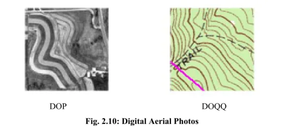
1. Images: These include aerial photos, scanned maps, satellite imagery, screen captures etc. Aerial photographs are the starting point for many mapping projects. Digital aerial photos are called Digital Orthophotos (DOP) or Digital Orthographic Quarter Quads (DOQQ). IGN France can provide aerial photos in ECW format: a format owned by ER Mapper (http://www.ermapper.com/). There are many sources of free DOP data all over the world, particularly in US e.g. the Microsoft TerraServer. DOP and DOQQ files (which are usually distributed on CDs due to their size) can also be purchased from a number of commercial vendors. For base maps different organizations provide digital topographic maps called Digital Raster Graphics (DRG).

DOP DOQQ

Fig. 2.10: Digital Aerial Photos

2. Vector Data: Traditionally geometric structures like lines, points, surfaces etc have been used to represent roads, streams, power lines, lakes, county boundaries, topographic lines, well sites, section corners, tower locations, etc., on a particular scale. In digital form (e.g.

Digital Line Graphs – DLG) this representation has the advantage of having a lot lesser heavy files than images. Moreover such a data can be resized without any loss of clarity. 3. Elevations: These are usually in the form of arrays or grid of terrain heights represented

usually by a wire frame or colors and recorded at regularly spaced horizontal intervals: the result being a Digital Elevation Model (DEM). DEM are used to create 3D images of a landscape by overlaying the corresponding 2D aerial photos or satellite images on them thus, for example, producing lighting effects to reveal hills, valleys etc. Many types of DEM are available to the public at various resolutions and scales. For example in USA the USGS provides DEM with 10m and 30m resolution and in France the IGN provides DEM with 50m resolution, i.e. one point for every 50 meters.

4. Spatial Databases: these include census data, resource inventory data, spatial event data, etc. In mapmaking such a data may sometimes be used to highlight some region(s) in the map, say, according to the population density. They may also help us forecasting changes in the terrain.

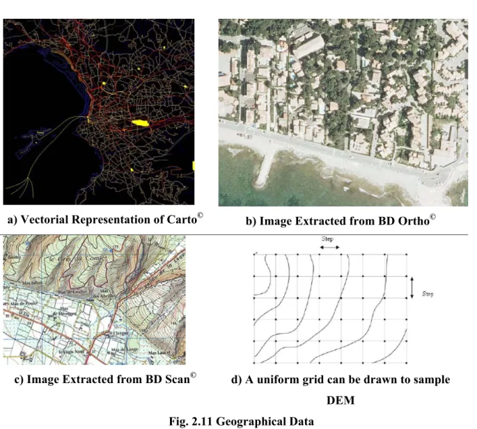
For 3D visualization, the former three types of data are essential. In our work we have relied on the data by IGN France which are:

• Vectorial data in the form carto©.

• Texure data in the form BD Ortho © and BD Scan ©. • DEM usually at 50m resolution

To obtain a three dimensional visualization, one has to link the texture with the terrain DEM. This link is allowed by geo-referencing coordinates (longitude / latitude) depending on the projection system used. These informations are usually stored in three different files (One for the DEM, one for the texture and one for the geo-referenced coordinates) [23].

Raster to Vector conversion is necessary for 3D visualization. This is done by scanning and saving the contour or topographic map in a raster image file format such as TIFF or JPEG. The raster image is converted to a vector format when contour lines are extracted and labeled by their elevation values: some specialized software can be utilized for this purpose. The vector data then can be saved in one of the many standard GIS formats, e.g. AutoCAD's DXF. These vectorized contour lines are used to create 3D digital elevation models (DEM’s) which is a

computer-intensive process. Interpolation algorithms are utilized to fill the space with elevation values using contours.

a) Vectorial Representation of Carto©

b) Image Extracted from BD Ortho©

c) Image Extracted from BD Scan© _{d) A uniform grid can be drawn to sample}

DEM Fig. 2.11 Geographical Data

Terrain representation implies to use two kinds of data combined for the visualization [2]:

• Height field data which correspond to the elevation of terrain (Figure 2.11d). These points are used to generate the geometry and are connected by triangles (Figure 2.12a).

• Different aerial photography can be computed in different spectrum (visible, infrared, etc). Theses ones are used to map 3D triangles previously computed (Figure 2.12b).

(a) 3D triangulated surface of the DEM. (b) Texture draped on the DEM Fig. 2.12: Example of 3D Visualization.

To obtain a 3D visualization, the simplest solution consists of using a uniform discretization of the terrain, which gives a good precision but leads to a quite large number of triangles. For example, if we use a uniform grid, with a step of 50 meters in each direction (see Fig. 2.11d) the department of the Bouches du Rhône in France corresponds to more than ten millions triangles (Around 13000 km²) which pertain to about 6 GB of data even if compressed. This implies a considerable cost, in terms of memory requirements, for the 3D visualization of a large area.

Many methods have been proposed in the literature to reduce the number of triangles provided by the uniform discretization, while preserving a good approximation of the original surface. One of the main approaches consists of obtaining an irregular set of triangles (TIN: Triangulated Irregular Network). A great deal of work has been done in order to create the TIN starting from a height field by using, for example, a Delaunay triangulation [24]. Hierarchical representations of these triangulations have been proposed, thus making it possible to introduce the concept of level of details [25]. Consequently one can obtain various levels of surfaces with an accuracy which is similar to a uniform grid but with a lower number of triangles. Another approach consists in breaking up the terrain in a set of nested regular grid of different level of details [26 - 28]. This approach has the advantage of allowing an optimal use of the capacities of the graphics cards and thus an increased speed of visualization. The main problem remains to connect the set of grids among themselves without cracks.

By draping a satellite/aerial image on a 3D terrain model, a realistic 3D model can be

created with the elevation and the surface texture. “First, the image region that covers the exact geographic area is defined and draped onto the surface of the terrain model. Then other images, even the original scanned map, can be used as the surface image to create a certain display effect.

The 3D display can be visualized and animated by changing the viewing angle and can be saved to a 3D file using formats such as” DEM, MNT (modèle numérique de terrain).

2.4 Related Works: Data Hiding in Wavelets

Many methods have been proposed for wavelet-based data hiding but few of these are compatible with the JPEG2000 scheme. According to [29] data hiding methods for JPEG2000 images must process the code blocks independently and that is why methods like inter-subband embedding [30], hierarchical multi-resolution embedding [31] and correlation-based methods [32] as well as non-blind methods are not recommended.

Xia et al [33] and Kundur and Hatzinakos [34] have embedded invisible watermarks by adding pseudorandom codes to the large coefficients of the high and middle frequency bands of DWT but the methods have the disadvantage of being non-blind.

Wang and Wiederhold [35] have proposed a system, they call WaveMark, for digital watermarking using Daubechies’ advanced wavelets along with the Hamming codes and smoothless analysis of the image. Highly smooth regions are the least preferred for their noticeable distortion and are applied with low strength watermarking.

Su, Wang and Kuo [36] have proposed a blind scheme to integrate EBCOT(Embedded Block Coding with Optimized Truncation) and image watermarking by embedding during the formation of compressed bit stream. The scheme is claimed to have robustness and good perceptual transparency.

In [37] watermark is embedded in the JPEG2000 pipeline after the stages of quantization and ROI scaling but before the entropy coding. For reliability purposes the finest resolution subbands have been avoided. A window sliding approach is adopted for embedding with the lowest frequencies having higher payload.

Piva et al [38] have proposed the embedding of image digest in a DWT based authentication scheme where the data is inserted in the layers containing the metadata. An N x N image is first wavelet transformed and the resultant LL subband is passed to DCT domain. The DCT coefficients are scaled down and of these some which are likely to be the most significant. After further scaling the DCT coefficients are substituted to the higher frequency DWT coefficients and the result is inverse DWTed to get the embedded image.

3. METHODOLOGY

As was discussed in the introductory chapter, the optimal real-time 3D visualization in a heterogeneous client-server environment requires synchronization and resolution scalability. The proposed solution was to reduce/compress the data as well as the number of files necessary for visualization. DWT, being an integral part of the JPEG2000 codec, was appropriate for us as its resolution scalability property perfectly coincided with the achievement of our scalability goal. We borrowed only the DWT aspect of the JPEG2000 in our work [1] and not followed the rest of the steps of the codec, e.g. for quantization we used just the floor function. As stated elsewhere that the lifting approach of wavelet transformation has its advantages over the convolution based approach, we adopted the former. As far as the reduction in the number of files was concerned we integrated those into one file by using a simple LSB based data hiding technique. LSB based approach was appropriate since high robustness was never the requirement as we were not guarding against some kind of malign attack.

3.1 Data Insertion

Our method, which is outlined in Fig. 3.1, consists of the following steps:

1. RGB to YCrCb: The texture image (in the PPM format) was passed from the RGB space to the luminance-chrominance space (YCrCb) thus resulting three different grayscale (PGM) images.

2. Wavelet Transformation: Both the DEM (PGM) and the three YCrCb planes were wavelet transformed at a desired level L. The DEM was both lossy (Daubechies - 9/7) and lossless (Daubechies - 5/3) transformed. Typically the texture images have considerably large sizes which call for utilizing every chance to reduce their sizes and that’s why for the YCrCb transformed texture images the lossy (Daubechies 9/7) transformed was exclusively employed.

3. Insertion: For the insertion of the DEM the luminance plane (Y), being the least sensitive of the other two planes, of the texture was used as a carrier. The DEM provided by the IGN France had 50m resolution, i.e. 1 altitude per 50m. Starting from the texture image of size, say, N² and a DEM file size m² a factor of insertion (E = m²/ N² coefficients/ pixel) was deduced. The texture image is thus must had to be divided into square blocks of size = 1/E pixels and every such block would be embedded with

one altitude coefficient. In this work, more specifically, corresponding to every 32x32 block of the texture image there were two bytes of altitude. Thus embedding was done by taking this correspondence into account, i.e. hiding in each 32x32 block its corresponding 2 bytes (16 bits) altitude. Since robustness and tamper resistance are not that important, i.e. as we are not guarding against attacks, LSB based insertions were made. Using a suitable seed, preferably prime, a pseudo-random number generator (PRNG) was initialized for earmarking the texture pixels thus hiding DEM with 1 bit of the later per earmarked texture pixel. Special care was taken to avoid collisions, i.e. not to assign the same pixel twice to embedding. Two things were taken into account. Firstly both the texture image and DEM must be at the same level of DWT transform at the time of embedding. This is not obligatory but for the start and for this work we persisted with this. Secondly there must have to be a correspondence in hiding the data and that’s why low frequencies were embedded in low frequencies and higher frequencies in higher.

4. Final Interleaved Image: The resultant interleaved Y plane along with the Cr and Cb plane gave us what we called the stego-image. The term stego is a misnomer over here since in the strict since it is not steganography. The resultant image can be transferred over a network channel from the server to clients. At the reception the DEM would be extractable even if part of this stego-image is transferred.

Depending on client’s resources the server may send the whole stego-image in which case the client would have to undo the whole process above and get very high quality visualization at the expense of the storage space. Otherwise a part of the stego-image is transmitted, i.e. lower frequencies (the higher frequencies have to be discarded and set to zero), thus giving lower quality but smaller size.

Fig. 3.1: Description of the Method Embedding DEM in the Texture Map

To asses the quality of an image with respect to some reference image the measure of PSNR (peak signal to noise ratio) has been employed which is given by:

MSE PSNR 2 10 255 log 10 =

Where MSE (the Mean Square Error) is a measure used to quantify the difference between the initial and the distorted/noisy image. Let pi represent the ith pixel of one image of size N and qi

that of other then:

N q p MSE N i i i

∑

− = − = 1 0 ) (

Fig. 3.2: Texture Image with the original scale.

3.2 Results and Discussion

The method was applied to a 2048 x 2048 pixels texture map of Bouches du Rhône France (Fig. 3.2) provided by the IGN associated with an altitude map of 64x64 coefficients (Fig. 3.3). Every altitude coefficient was coded in 2 bytes and associated with a 32x 32 texture block.

Fig. 3.3: Altitude (DEM) with the original scale

In the rest of this discussion for purpose of comparison and explanation we will resize all the images to the same size and hence they would not be according to the original scale. Hence images of Fig. 3.2 and 3.3 are re-shown in Fig. 3.4.a and 3.4.c. Fig 3.4b shows a magnified/detailed part (128x128 pixels) of the texture image.

We have used lossy DWT for the Texture image and lossless DWT for the DEM data up to level 3. The resultant transformed images are shown in Fig. 3.4 for level 1 and in Fig. 3.5 for level 3. Keeping synchronization in view, data embedding has been done for any level L in 3L+1 steps corresponding to the number of subbands: hence for level 1 it is in four steps (corresponding to LL, LH, HL and HH subbands) - Fig. 3.4a – and for level 3 insertion is in 10 steps ( Fig. 3.5a).

For each of the three levels the difference between the wavelet transformed luminance image before and after insertion of data corresponded to a PSNR of around 69.20dB which implies no marked loss of quality. This is understandable since we embedded just 16 bits per 32 byte by 32 bytes, i.e. 1 bit per 64 bytes.

a. b.

c.

a. b.

Fig. 3.5 – DWT at level 1: a. Texture, b. Altitude

a. b.

Table 3.1 summarizes the results obtained when images were reconstructed from the images of approximation, i.e. lowest frequency subband (e.g. LL for level 1), at various levels. Note that if we utilize all the data for DWT-1 we get a PSNR of 37.32 dB for the resultant texture image which is understandable since we had applied the lossy transform to texture image. For altitude the value is infinity since lossless transform was applied to it. Fig. 3.7 shows the results in case where the approximation image from an already embedded level 3 image is inverse wavelet transformed. By carrying out the difference between this rebuilt texture image of Fig 3.7a and the original texture we obtain a PSNR of 20.90 dB. The detailed portion of Fig 3.4b can be compared with that of rebuilt one illustrated in Fig. 3.7b. The difference is obvious but this difference is small given the fact that a very small portion of data has been employed. From the image of approximation of level 3, if we carry out the extraction of the hidden data followed by an inverse DWT, we obtain the illustrated altitude image of Fig. 3.7c. The PSNR between original altitude and the rebuilt is then 29.25 dB. Note that while using the image of approximation of the level 3 we needed only 1.6% of the initial data. For level 1 and 2 the corresponding altitude images are given in Fig. 3.8.

Resolution Level 0 * 1 2 3

% Transmitted Data 100% 25% 6.25% 1.6%

Texture (dB) _37.62 26.54 22.79 20.90

Altitude (dB) ∞ 40.37 33.51 29.25

MSE Altitude (m²) 0 5.97 29.00 77.37

* All the data utilized for DWT-1

Table 3.1: Results obtained after the extraction and reconstruction as a function of the data utilized

a. b.

c.

Fig 3.7 – Reconstruction of the images from the image of approximation at Level 3: a) Texture, b) Magnified part of texture corresponding to that of Fig.3.4.b and c)

a. b.

Fig. 3.8 – Reconstruction of altitude map from the approximation image of: a) level 2 and b) level 1.

The rebuilding of the 3D DEM for the image of approximation from various levels (0-3) resulted in the images of Fig. 3.9. By draping the texture on the DEM Fig. 9.a and 9.b allow us to compare the final result between visualization with all the data and visualization only with level 3 composed of 1.6% of the initial data.

Fig 3.9 – 3D visualization of the Altitude from the lowest frequency subband: a) with all the

a. b.

4. CONCLUSION

In this work we adopted the strategy of using the orthophotograph as a carrier for hiding the corresponding DEM data on which it would be draped for 3D visualization. Within the client-server framework, that we want to establish, we can thus synchronize this information, thus avoiding any error related to an erroneous combination of the data or a lack thereof due to their transfer. The use of wavelets provided us the resolution scalability thus making it possible to transfer the levels necessary for an optimal visualization according to the choice or resources of the user. Moreover our method is integrable with the JPEG2000 coder, since we have used the types of wavelet supported by the standard, which means that any JPEG2000 supported image viewing softwares can be used for the visualization of the texture. The results have been encouraging and with a data as small as 1.6% of the original (that is the approximation image from level 3) we were able to get fairly good quality visualization.

Despite having interesting results we would, in the continuation of our work, wish to set up a finer DEM storage. We solely concentrated on wavelets supported by JPEG2000 but not the other aspects of the standard. Hence it may eventually prove beneficial to take into account the JPEG2000 standard as a whole and, to standardize the results, utilize an open source popular implementation e.g. OpenJPEG (http://www.openjpeg.org/), for experimentation instead of our own implementation used in this work. Even in the domain of wavelets one can go further and, for example, explore the geometrical wavelets. We will also study the possibility of no more using a uniform grid at various levels of details, thus allowing us to decrease the number of triangles necessary for a good representation of the terrain wherever variations in the terrain are not very important. For data hiding just the luminance plane was used as a carrier because of its lower sensitivity and it remains to be seen whether it would work with the two chrominance planes or not. For the moment the altitude data is small but with the possibility of finer but larger data in the future it would be desirable to evaluate the data hiding capacities and eventually explore the chrominance planes for embedding.