Experimental study of Elementary Cellular Automata dynamics using the density parameter

HAL Id: hal-01183311

https://hal.inria.fr/hal-01183311

Submitted on 11 Aug 2015

HAL is a multi-disciplinary open access

archive for the deposit and dissemination of

sci-entific research documents, whether they are

pub-lished or not. The documents may come from

teaching and research institutions in France or

abroad, or from public or private research centers.

L’archive ouverte pluridisciplinaire HAL, est

destinée au dépôt et à la diffusion de documents

scientifiques de niveau recherche, publiés ou non,

émanant des établissements d’enseignement et de

recherche français ou étrangers, des laboratoires

publics ou privés.

dynamics using the density parameter

Nazim Fatès

To cite this version:

Nazim Fatès. Experimental study of Elementary Cellular Automata dynamics using the density

parameter. Discrete Models for Complex Systems, DMCS’03, 2003, Lyon, France. pp.155-166.

�hal-01183311�

Experimental study of Elementary Cellular

Automata dynamics using the density

parameter

Nazim Fat`es

1

46, all´ee d’Italie - 69 364 Lyon Cedex 07 - France.

Nazim.Fates@ens-lyon.fr

Classifying cellular automata in order to capture the notion of chaos algorithmically is a challenging problem than can be tackled in many ways. We here give a classification based on the computation of a macroscopic parameter, the d-spectrum, and show how our classifying scheme can be used to separate the chaotic ECA from the non-chaotic ones.

Keywords: Cellular Automata, Classification, Discrete Dynamical Systems, Density

1

Introduction

In [Gut89] Howard Gutowitz writes :

“A fundamental problem in theory of cellular automata is classification. A good classification divides cellular automata into groups with meaningfully related properties. In general there are two types of classifications : phenotypic and genotypic. A phenotypic classification divides a population into groups according to their observed behaviour. A genotypic classification divides a population into groups accord-ing to the intrinsic structure of the entities in the population.”

In 1984, the first phenotypic classification has been proposed by Wolfram [Wol84] dividing cellular automata (CA) according to their “observed dynamics”. This classification was very important since it motivated numerous researches but was at the same time criticised by many authors on grounds that no formal definitions of the classes were given.

In 1989, Culik and Yu in [ ˇCPY89] proposed a formal definition of the classes according to some asymp-totic behaviour of the cellular automaton and showed the undecidability of the classifying scheme.

The class of CA that has drawn much attention is the class of the 256, 2-state 3-neighbours CA, or so-called Elementary CA (ECA). An interesting axis of investigation was the application of topological analysis theory to cellular automata. In 1998, Cattaneo et al. in [CFM99] proposed a genotypic classi-fication of all of the 256 ECA that has the advantage to rely on formal definitions as well as theoretical justifications.

In this work, we propose a phenotypic classification based on the observation of the statistical evolu-tion of a “macroscopic parameter”, the density, that can easily be computed and that is the result of the aggregation of the data obtained at the cell scale. We then compare the results obtained experimentally to Wolfram’s and Cattaneo’s classification and examine the similarities and differences with both authors.

2

Classifying ECA dynamics

2.1

Position of the problem

The finite ECA have an advantage over CA with higher states or dimension : their dynamics can be easily represented using space-time diagrams in which the cell array x(t) is represented by a horizontal sequence

of light and dark cells that symbolise the states 0 and 1 and time as the vertical axis.

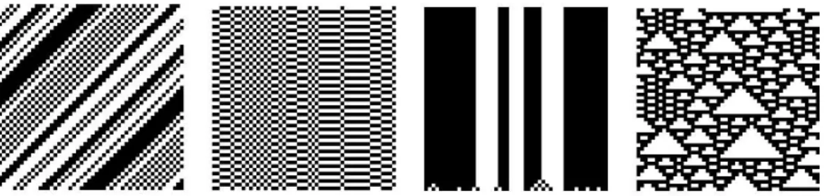
Fig. 1 represents 4 examples of space-time diagrams. Intuition leads to consider the first three as very regular and the last one as more irregular, or more “chaotic”.

Fig. 1. Time goes from bottom to top, space-time diagrams are displayed for the rules 170 , 51 , 232 ,

126 (see§2.3 for the rule encoding).

The purpose of our classification is to discriminate the ECA that produce “chaotic looking” space-time diagrams from the others. From a theoretical point of vue, the work of Culik & al. [ ˇCPY89] showed that the problem of knowing, for a given CA, whether every (infinite) configuration evolves to a global (unique) fixed point in a finite number of steps, is undecidable. A classifying scheme can thus be shown undecidable even with a classification defined in a very simple an intuitive way.

From the work of Mazoyer and Rapaport [MR99], we know that it stills remains undecidable whether every circular (thus finite) configuration of a given one-dimensional CA evolves to the same fixed point. This result is ever more convincing as it shows that a classification in which we demand a given propriety to be verified for all of the configurations can be undecidable even when the classes are defined in very simple and intuitive ways.

An alternative approach, proposed in [Wol84] is to classify each ECA by looking at its behaviour and judging by eye whether most of the CA behaviour is periodic or chaotic. The goal of this work is to present a classification which tries to algorithmically capture the informal notion of “most of the CA behaviour is periodic or chaotic” in order to have a classifying scheme that is effective and that can be implemented to test the 256 ECA.

2.2

The idea behind our classification

To characterise formally the qualitative behaviour of a space-time diagram, several macroscopic param-eters such as spatial or time entropy, Lyapunov exponent, etc. have been proposed. To our knowledge, none of them have been shown to be fully satisfying in regard to accounting for the “chaotic behaviour” of a CA. As far as the ECA space is concerned, we can say that we found very few tables in which the 256 ECA are exhaustively classified according to the computation of a macroscopic parameter.

One difficulty for establishing such an exhaustive study might be that the computation of a macroscopic parameter (e.g. entropy) is too slow and thus cannot be performed for a great number of initial conditions and for all the 256 ECA. The density parameter, i.e. the number of 1’s divided by the total number of cells, is an efficiently computed macroscopic parameter. We wondered whether it could be used to characterise the notion of chaos in the evolution of a CA.

An investigation of the statistical evolution of this parameter lead us to make the following observation:

• In a chaotic-looking ECA, for almost all of the initial conditions, the density parameter evolves with

large statistical distributions.

• In a periodic-looking ECA, for almost all of the initial conditions, the evolution of the density

stabilises after a transient time and enters into a cycle of small length, i.e. less or equal to 3. This work is aimed at testing experimentally the validity of this observation and deriving a classification of the ECA from it.

2.3

General definitions

The cellular automata we here study are objects which act on a one-dimensional finite lattice of cells, where each cell is assigned a state in A= {0, 1}. Let n be the size of the lattice, a configuration is an

assignment of states to the cells of the lattice, it is a word in An, denoted x= x0· · · xn−1, with xi∈ A. The

set of all possible words of size n, An, is the phase space. The configurations are cyclic and all indices have to be considered in Z/nZ. Our finite 1D lattice is then a ring and we have x−1= xnand xn= x0.

An ECA is a function f : A3→ A , called the local transition rule, to which we associate the global

transition function Ff : An→ Andefined by :

Ff(x0· · · xn−1) = y0· · · yn−1

where

yi= f (xi−1, xi, xi+1)

Following [Wol84] we associate to each ECA f its code :

W( f ) = f (0, 0, 0) · 20_{+ f (0, 0, 1) · 2}1_{+ · · · + f (1, 1, 0) · 2}6_{+ f (1, 1, 1) · 2}7

An ECA f having the code R= W ( f ) is denoted by R and we do not distinguish the rule from its code.

D

of size n. We denote by x(t) = FRt(x) the tthiterate of F on x, with x(0) = x and call an orbit the function

x(t).

Since the phase space is finite, every orbit is ultimately periodic, so:

2.4

Definition of the

d

-spectrum

The density is the function d : An_{→ [0, 1] such that d(x) =} #1(x)

n where #1(x) denotes the number of 1 in

x and n is the size of the configuration x.

For a given DDS

D

whose image under the rule F is invariant, i.e., such that F(C) = C. The transient time of the orbit, T (x),

is the size of the complement T of C in H.

The shift-invariant macroscopic parameter that we use as the discriminating factor of our classification is called the d-spectrum of x, denoted byτ(x) and defined by:

τ(x) = |{d(x), x ∈ C}|

It measures the number of different densities that appear in the cycle of an orbit. This number is clearly bounded by n+ 1, as : ∀x ∈ An_{, d(x) ∈ F} n= { k n, k ∈ [0, n]}

3

Experimental protocol

We present here the protocol we have used to perform the numerical experiments.

3.1

d

-spectrum estimation

For a given DDS

D

The estimation is performed by letting the dynamical system

D

then measure the evolution of the density parameter during Tsamplingtime steps. Ttransientand Tsamplingare

two constants that are chosen as an approximation of the transient time T(x) and the cycle length |C|. This

results in the application of the following algorithm :

Let h be an array of integers with index in [0..n], initialise h to 0

initialise τ˜(x) to 0

For t ← 1 to Ttransient+ Tsampling do x ← F(x)

if t > Ttransient then h(d(x).n)++ For i ← 0 to n do

if h(i) 6= 0 then τ˜(x)++ .

At the end, h is the array containing in place i the number of times density _ni has been observed. The numerical d-spectrum ˜τ(x) is computed as being the number of non-zero values of the histogram h.

3.2

Class estimation

In this work, we propose to estimate experimentally the number of different densities obtained in the orbits when starting from almost all of the initial conditions. Since the computation of all initial conditions is impossible in practice, we have to start from a limited set I⊂ An _{of initial conditions to perform the}

computation.

For a DDS

D

all the values in TIare smaller than Kpfor a periodic-looking rule. Similarly, there should exist a constant

Kcsuch that Kc> kpand such that all the values in TIare greater than Kpfor a chaotic-looking rule.

We thus apply the following classifying scheme :

• R is in class P if TI⊂ [1, Kp],

• R is in class C if TI⊂ [Kc,∞[,

• R is in class H if it is neither in P nor in C.

To test our conjecture, we expect the classifying algorithm to fulfil the following requirements :

• The results can be obtained in a reasonable computing time. • The algorithm produces the same results for different runs. • The cardinal of the class H is small.

• The results are stable for different n provided that n is big enough.

So, we have to find a set of initial conditions I, and two constants Kpand Kc, such that the requirements

stated above are verified.

3.3

How to fix the the constants

3.3.1

The case of

n

,

T

,

T

The ring size n should be chosen as large as possible in order to guarantee that the asymptotic behaviour of the orbits no longer depends on n. The limiting factor in the choice of n is the computing abilities available for the numerical experiments. It has been shown experimentally that the values of the average transient time Ttransient and the average cycle length|C| grow exponentially with D for some chaotic-looking rules

[Gut91].

We tune the value of Ttransientby ensuring that for all the periodic-looking ECA, for all initial conditions,

the computed ˜τ() is no longer varying for higher values of Ttransient. While doing the experiments, we

observed that the value of Tsamplinghas little influence on the results as long as Tsampling≥ n, so we simply

take Tsampling= n .

3.3.2

The case of

I

Let us recall that the definition of our classification is based on the estimation of the behaviour of a given rule on almost all of the initial conditions. We thus have to a assign a precise meaning to the expression “almost all”. Clearly, we cannot take all the phase space Anas the set of initial conditions I since we know that Ancontains some configurations which behaviour is not dependent on the rule. However, we cannot exclude too many configurations in Anwithout taking the risk that I is not representative of almost all the configurations of An. The criteria we take in this paper is to say that a set configurations Vndefined for

every n, is representative if limn→∞|V₂nn| = 1; i.e., if the limit set of Vnhas a measure 1 with the uniform

measure.

For example, we can notice that whatever the rule and whatever the ring size, we have : τ( ¯0) ≤ 2,

containing the configuration ¯0, any rule verifies 1∈ TIor 2∈ TI (see§3.2 for the definition of TI). This

implies, according to our definitions of the classes, that no rule would ever be classified in C if its sampling set I contains ¯0. So, we have to exclude the configurations ¯0 and ¯1 from I just as well as other special configurations.

In this work, we take the following set as a representative set of initial conditions:

Vn= {x ∈ An, 11 ⊂ x and 00 ⊂ x}

Vnis the set of configurations in which not all the 1’s or 0’s are isolated. The motivation for using(Vn)n∈N comes from the fact that for some ECA, such as rule 180, any configuration in which all the 1s are isolated (surrounded by 0’s) or all the 0’s are isolated (surrounded by 1’s) have a large d-spectrum indicating a chaotic behaviour, whereas all other configurations have small d-spectrum indicating a periodic behaviour. A more detailed description of such “strange” behaviours can be found in [CM98].

The most natural way of constructing I is to select configurations randomly with a uniform sampling in

Anand discard the configurations which are not in Vn. This would be correct and satisfying according to

our criteria but we can notice that the greatest part of the selected configurations would have density close to 1/2. In order to have different densities represented, we take a set of densities D= {d1, d2, · · · , dk} and

build I as follows:

I= [ d∈D

INs(d)

where INs(d) denotes a subset of Vn, constructed with Nsinitial configurations of density d, that is words resulting from the concatenation of letters that have probability d to be 1 and probability 1− d to be 0.

3.3.3

The case of

K

,

K

In order to guarantee that P and C are disjoint, we require that Kc> Kp. Recall that we have conjectured

that Kp= 3 would be suitable and that we want the class H to have a cardinal as small as possible.

3.4

Results

For n= 50, it appears empirically that Ttransient= 200 was suitable in order to have the stability of the

results. For the results here provided, we take n= 100 and Ttransient= 1000.

Concerning the initial condition sampling, we always take 150 initial conditions for each ECA, with

D= {0.3, 0.4, 0.5, 0.6, 0.7} and Ns= 30.

Because we conjectured that non-chaotic ECA would produce d-spectra less or equal to 3, we take

Kp= 3 for all n. To detect the chaotic rules, we observe that taking Kc= 4 for n = 50 and Kc= 7 for

n= 100 provides a classification which fulfils the criteria of §3.2.

Using this numerical values, it appears that the output of the algorithm is stable when we run it several times. However, some particular rules (e.g rule 9) are sometimes classified as H instead of P. This indicates that not all orbits enter into a cycle after 1000 steps and that Ttransient should be

cho-sen bigger in order to guarantee the stability of the results. Unfortunately, we here reach the limit of our computing abilities as the number of elementary steps (application of the rule) is given by :

nop= 256 · Ns· (Ttransient+ Tsampling) · n = 256 · 150 · 1200 · 100 ∼ 1010.

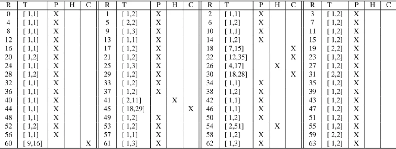
The numerical results are shown in the table at the end of the article. ECA are given with rule number R, the smallest interval T that contains TIand the class. We find out that 204 ECA are P, 30 ECA are C

and 22 ECA are H. This results confirms that Kp= 3 and Kp= 7 is a suitable choice : t allows to fully

discriminate 204+30 ECA as P or C, letting the 22 ECA in H with an undetermined behaviour. Thus, a natural clusterisation of the ECA space seems to emerge.

3.5

Symmetries of the ECA space

One means of verification of the consistence of the table is the use of symmetries. Indeed, for any ECA defined by local transition function f , we can associate the following ECA:

1. f0, the reflected rule of f defined by :

∀(x−1, x0, x1) ∈ A3, f0(x−1, x0, x1) = f (x1, x0, x−1).

2. f∗, the conjugate rule of f defined by :

∀(x−1, x0, x1) ∈ A3, f∗(x−1, x0, x1) = [ f (x∗−1, x∗0, x∗1)]∗. where∗ denotes the operation of changing 0’s into 1’s and 1’s into 0’s.

3. f0∗, the reflected conjugate rule of f defined by :

∀(x−1, x0, x1) ∈ A3, f0∗(x−1, x0, x1) = [ f (x∗1, x∗0, x∗−1)]∗.

As f , f∗, f0and f0∗are obtained using symmetries (they are isometrically conjugate), we expect that the classifying scheme attributes the same class to each of this rule. This requirement appears to be verified experimentally with our classifying scheme.

4

Analysis of the results

We here compare the numerical results to two different classifications.

4.1

Comparison with Cattaneo’s et al. classification

In [CFM99] Cattaneo et al. provide a table in which the 256 ECA are classified according to the properties of their transition table. This genotypic classification is based on topology and uses three main classes

C1, C2, C3formally defined for an infinite one-dimensional lattice. The three main classes are subdivided into smaller classes using some particular proprieties of the local rule. Some of the defined sub-classes explicitly group rules that have the same asymptotic behaviour whereas some other sub-classes cannot allow qualitative predictions to be made.

For example, if we look at a sub-class which is characterised by “Periodic-1 attractor containing reach-able ¯0”, we expect all the orbits to reach the ¯0 configuration and to have a d-spectrum of 1. Indeed, we find that all rules of this subclass are P in our classification (rules 72, 104, 200, 232, 4, 36, 132, 164).

Some other classes provided in Cattaneo’s et al. classification are not regrouping ECA that have a homogeneous behaviour. The most interesting case of non homogeneity appears for the rules 18, 22, 26, 82, 94, 122, 126, 146, 182, 218 which are classified in the same sub-class denoted “sub 90”. Using our classification, we find that:

• rules 26, 82, 94 are H,

• rule 218 is P.

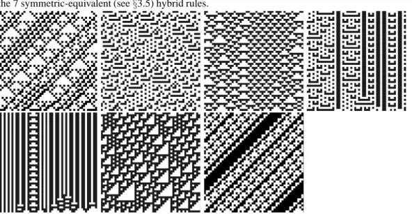
Indeed, one can verify experimentally that rule 218 seems to always converge (quickly) to a fixed point. On the other hand rules 18, 22, 122, 126, 146, 182 do exhibit a chaotic-looking behaviour. Rule 26 and 82, which are isometrically conjugate, have a behaviour that cannot be clearly identified as periodic or chaotic: the space-time diagrams it produces are reminiscent of the shift (rule 170 see fig. 1) but shows some kind of “complexity” (see fig. 2). The rule 94 appears as an exception as it has a very stable signature having TI⊂ [1, 6] and could be classified in P with Kp= 6.

It thus appears that the predictions given by topological analysis are verified experimentally and that the numerical results we provide might be useful to allow a finer analysis of the classes for which no theoretical prediction can be made.

Fig. 2. Some space-time diagrams obtained with the rules 26, 41, 54, 73, 94, 110, 154 which represent the 7 symmetric-equivalent (see§3.5) hybrid rules.

4.2

Comparison with Wolfram’s phenotypic classification

The classification proposed by Wolfram in [Wol84] divides the CA space into 4 classes : Class W1 evolution of the CA leads to homogeneous stable configuration Class W2 evolution of the CA leads to a set of separated simple or periodic structures

Class W3 evolution of the CA leads to a chaotic pattern

Class W4 evolution leads to complex localised structures sometimes long-lived

Concerning class W4, which is the class of the most “complex” ECA, the fuzziness of the definition does not allow to classify an ECA as W4 without making a somehow arbitrary choice. It has been con-jectured that class W4 is constituted out of the ECA that are capable of universal computation, that is, that are able to calculate the result of any function defined algorithmically. So far, only rule 110 (and its isometrically conjugated rules 137,124,193) was clearly identified having this ability (see [Wol02]). Rule

54 is also another good candidate for having the computation universal ability but so far no evidence was given. As there is no “official” Wolfram classification, each author is allowed to make his own and we compared our results to the Wolfram classification given in [CFM99].

We observe that that any ECA that we classify P is classified W1 or W2, and that any ECA that we classify C is classified W3. For the ECA that we classify H, we find out that some of them, e.g rule 94, are W2 whereas some others, e.g rule 26, are W3. This agreement confirms the

It is worth noticing that rule 54 and rule 110 are both in class H. Recall that our class H is defined as the class of ECA that have a set of d-spectrum that is neither all inside[1, Kp] nor inside [Kc,∞[. Thus, an

ECA which is H has the ability to produce small spectrum, like non-chaotic ECA, as well as large d-spectrum, like chaotic ECA. These particular ECA exhibit a behaviour that we can qualify to be “hybrid”. Their characterisation using the d-spectrum might confirm the idea that rules which exhibit a “complex” behaviour are situated in a transition zone in rule space, between chaotic ECA and ordered ECA [LPL90].

5

Conclusion and perspectives

We proposed to use an efficiently computable macroscopic parameter, the d-spectrum, to classify the 256 rules of the ECA space. The most important features of the classifying scheme might be its coherence with other classifications and its ability to find “complex” rules of the ECA space (rules 54 and 110).

Because we have worked on finite lattices, the classificiation operates on couples rule/lattice and might depend on the size of the lattice. In order to prove the membership of a rule for any ring size, it might be worth to formalise the classification and to obtain theoretic results.

The characterisation of chaos we proposed for the ECA can be generalised to cellular automata with higher number of states and higher dimensions and even to objects which are not cellular automata such as boolean networks. One may wonder how the constants Tsamplingand Ttransientvary for such objects and

whether a clusterisation of the space can still be exhibited. Another axis of investigation is to use this macroscopic parameter to characterise other concepts related to cellular automata, such as the “robust-ness” of a cellular automaton, that is its ability to keep its behaviour constant when submitted to little perturbation of its topology or synchronicity.

References

[CFM99] G. Cattaneo, E. Formenti, and L. Margara. Topological chaos and ca. In M. Delorme and J. Mazoyer, editors, Cellular Automata - A Parallel model, volume 460, pages 213–259. Kluwer Academic Publishers, 1999.

[CM98] G. Cattaneo and L. Margara. Generalized sub-shifts in elementary cellular automata: The ”strange case” of chaotic rule 180. Theorectical Computer Science, 201(1-2):171–187, 1998. [ ˇCPY89] K. ˇCulik, Y. Pachl, and S. Yu. On the limit sets of cellular automata. SIAM Journal of

Comput-ing, 18:831–842, 1989.

[Gut89] H. Gutowitz. Mean field vs. wolfram classification of cellular automata (unpublished). Avail-able on : http://www.santafe.edu/˜xhag, 1989.

[Gut91] H. Gutowitz. Transients, cycles and complexity in cellular automata. Physical Review A, 44(12):7881–7884, December 1991.

[LPL90] W. Li, N. Packard, and C. G. Langton. Transition phenomena in CA rule space. Physica D, 45:77, 1990.

[MR99] J. Mazoyer and I. Rapaport. Global fixed points attractors of circular cellular automata and periodic tilings of the plane : undecidability results. Discrete Mathematics, 199:103–122, 1999.

[Wol84] S. Wolfram. Universality and complexity in cellular automata. Physica D, 10:1–35, 1984.

[Wol02] S. Wolfram. A new kind of science. Wolfram Media Inc., 2002.

Tab. 1: Experimental results for: X= 100, Ns= 30, D = {0.30, · · · , 0.70}, Ttransient= 1000 , Tsampling= 100, Kp= 3, Kc= 7

R T P H C R T P H C R T P H C R T P H C 0 [ 1,1] X 1 [ 1,2] X 2 [ 1,1] X 3 [ 1,2] X 4 [ 1,1] X 5 [ 2,2] X 6 [ 1,2] X 7 [ 1,2] X 8 [ 1,1] X 9 [ 1,3] X 10 [ 1,1] X 11 [ 1,2] X 12 [ 1,1] X 13 [ 1,1] X 14 [ 1,2] X 15 [ 1,2] X 16 [ 1,1] X 17 [ 1,2] X 18 [ 7,15] X 19 [ 2,2] X 20 [ 1,2] X 21 [ 1,2] X 22 [ 12,35] X 23 [ 1,2] X 24 [ 1,1] X 25 [ 1,3] X 26 [ 4,17] X 27 [ 1,2] X 28 [ 1,2] X 29 [ 1,2] X 30 [ 18,28] X 31 [ 2,2] X 32 [ 1,1] X 33 [ 1,2] X 34 [ 1,1] X 35 [ 1,2] X 36 [ 1,1] X 37 [ 1,2] X 38 [ 1,2] X 39 [ 1,2] X 40 [ 1,1] X 41 [ 2,11] X 42 [ 1,1] X 43 [ 1,2] X 44 [ 1,1] X 45 [ 18,29] X 46 [ 1,1] X 47 [ 1,2] X 48 [ 1,1] X 49 [ 1,2] X 50 [ 1,2] X 51 [ 1,2] X 52 [ 1,2] X 53 [ 1,2] X 54 [ 2,51] X 55 [ 1,2] X 56 [ 1,1] X 57 [ 1,1] X 58 [ 1,2] X 59 [ 2,2] X 60 [ 9,16] X 61 [ 1,3] X 62 [ 1,3] X 63 [ 1,2] X

R T P H C R T P H C R T P H C R T P H C 64 [ 1,1] X 65 [ 1,3] X 66 [ 1,1] X 67 [ 1,3] X 68 [ 1,1] X 69 [ 1,1] X 70 [ 1,2] X 71 [ 1,2] X 72 [ 1,1] X 73 [ 2,30] X 74 [ 1,1] X 75 [ 17,27] X 76 [ 1,1] X 77 [ 1,1] X 78 [ 1,1] X 79 [ 1,1] X 80 [ 1,1] X 81 [ 1,2] X 82 [ 3,17] X 83 [ 1,2] X 84 [ 1,2] X 85 [ 1,2] X 86 [ 18,27] X 87 [ 1,2] X 88 [ 1,1] X 89 [ 17,28] X 90 [ 10,18] X 91 [ 1,2] X 92 [ 1,1] X 93 [ 1,1] X 94 [ 1,6] X 95 [ 1,2] X 96 [ 1,1] X 97 [ 2,4] X 98 [ 1,1] X 99 [ 1,1] X 100 [ 1,1] X 101 [ 16,26] X 102 [ 11,17] X 103 [ 1,3] X 104 [ 1,1] X 105 [ 10,17] X 106 [ 16,31] X 107 [ 2,4] X 108 [ 1,2] X 109 [ 3,29] X 110 [ 2,19] X 111 [ 1,3] X 112 [ 1,1] X 113 [ 1,2] X 114 [ 1,2] X 115 [ 1,2] X 116 [ 1,1] X 117 [ 1,2] X 118 [ 1,3] X 119 [ 1,2] X 120 [ 17,29] X 121 [ 3,4] X 122 [ 7,28] X 123 [ 1,2] X 124 [ 2,19] X 125 [ 1,3] X 126 [ 7,28] X 127 [ 1,2] X 128 [ 1,1] X 129 [ 7,30] X 130 [ 1,1] X 131 [ 1,3] X 132 [ 1,1] X 133 [ 1,6] X 134 [ 1,2] X 135 [ 17,28] X 136 [ 1,1] X 137 [ 2,18] X 138 [ 1,1] X 139 [ 1,1] X 140 [ 1,1] X 141 [ 1,1] X 142 [ 1,2] X 143 [ 1,2] X 144 [ 1,1] X 145 [ 1,3] X 146 [ 7,14] X 147 [ 2,51] X 148 [ 1,2] X 149 [ 18,30] X 150 [ 9,15] X 151 [ 22,35] X 152 [ 1,1] X 153 [ 10,18] X 154 [ 3,19] X 155 [ 1,2] X 156 [ 1,2] X 157 [ 1,2] X 158 [ 1,2] X 159 [ 1,2] X 160 [ 1,1] X 161 [ 7,28] X 162 [ 1,1] X 163 [ 1,2] X 164 [ 1,1] X 165 [ 9,18] X 166 [ 2,22] X 167 [ 4,19] X 168 [ 1,1] X 169 [ 16,29] X 170 [ 1,1] X 171 [ 1,1] X 172 [ 1,1] X 173 [ 1,1] X 174 [ 1,1] X 175 [ 1,1] X 176 [ 1,1] X 177 [ 1,2] X 178 [ 1,2] X 179 [ 1,2] X 180 [ 2,17] X 181 [ 3,14] X 182 [ 7,15] X 183 [ 7,15] X 184 [ 1,1] X 185 [ 1,1] X 186 [ 1,1] X 187 [ 1,1] X 188 [ 1,1] X 189 [ 1,1] X 190 [ 1,1] X 191 [ 1,1] X 192 [ 1,1] X 193 [ 2,21] X 194 [ 1,1] X 195 [ 10,18] X 196 [ 1,1] X 197 [ 1,1] X 198 [ 1,2] X 199 [ 1,2] X 200 [ 1,1] X 201 [ 1,2] X 202 [ 1,1] X 203 [ 1,1] X 204 [ 1,1] X 205 [ 1,1] X 206 [ 1,1] X 207 [ 1,1] X 208 [ 1,1] X 209 [ 1,1] X 210 [ 2,15] X 211 [ 1,2] X 212 [ 1,2] X 213 [ 1,2] X 214 [ 1,2] X 215 [ 1,2] X 216 [ 1,1] X 217 [ 1,1] X 218 [ 1,1] X 219 [ 1,1] X 220 [ 1,1] X 221 [ 1,1] X 222 [ 1,1] X 223 [ 1,1] X 224 [ 1,1] X 225 [ 16,29] X 226 [ 1,1] X 227 [ 1,1] X 228 [ 1,1] X 229 [ 1,1] X 230 [ 1,1] X 231 [ 1,1] X 232 [ 1,1] X 233 [ 1,1] X 234 [ 1,1] X 235 [ 1,1] X 236 [ 1,1] X 237 [ 1,1] X 238 [ 1,1] X 239 [ 1,1] X 240 [ 1,1] X 241 [ 1,1] X 242 [ 1,1] X 243 [ 1,1] X 244 [ 1,1] X 245 [ 1,1] X 246 [ 1,1] X 247 [ 1,1] X 248 [ 1,1] X 249 [ 1,1] X 250 [ 1,1] X 251 [ 1,1] X 252 [ 1,1] X 253 [ 1,1] X 254 [ 1,1] X 255 [ 1,1] X