Cortical Pitch Regions in Humans Respond Primarily to Resolved Harmonics and Are Located in Specific Tonotopic Regions of Anterior Auditory Cortex

Cortical Pitch Regions in Humans Respond Primarily

to Resolved Harmonics and Are Located in Specific

Tonotopic Regions of Anterior Auditory Cortex

The MIT Faculty has made this article openly available.

Please share

how this access benefits you. Your story matters.

Citation

Norman-Haignere, S., N. Kanwisher, and J. H. McDermott. “Cortical

Pitch Regions in Humans Respond Primarily to Resolved Harmonics

and Are Located in Specific Tonotopic Regions of Anterior Auditory

Cortex.” Journal of Neuroscience 33, no. 50 (December 11, 2013):

19451–19469.

As Published

http://dx.doi.org/10.1523/jneurosci.2880-13.2013

Publisher

Society for Neuroscience

Version

Final published version

Citable link

http://hdl.handle.net/1721.1/89140

Terms of Use

Article is made available in accordance with the publisher's

policy and may be subject to US copyright law. Please refer to the

publisher's site for terms of use.

Systems/Circuits

Cortical Pitch Regions in Humans Respond Primarily to

Resolved Harmonics and Are Located in Specific Tonotopic

Regions of Anterior Auditory Cortex

Sam Norman-Haignere,

_{Nancy Kanwisher,}

_{and Josh H. McDermott}

1_{McGovern Institute for Brain Research and}2_{Department of Brain and Cognitive Sciences, Massachusetts Institute of Technology, Cambridge,} Massachusetts 02139

Pitch is a defining perceptual property of many real-world sounds, including music and speech. Classically, theories of pitch perception

have differentiated between temporal and spectral cues. These cues are rendered distinct by the frequency resolution of the ear, such that

some frequencies produce “resolved” peaks of excitation in the cochlea, whereas others are “unresolved,” providing a pitch cue only via

their temporal fluctuations. Despite longstanding interest, the neural structures that process pitch, and their relationship to these cues,

have remained controversial. Here, using fMRI in humans, we report the following: (1) consistent with previous reports, all subjects

exhibited pitch-sensitive cortical regions that responded substantially more to harmonic tones than frequency-matched noise; (2) the

response of these regions was mainly driven by spectrally resolved harmonics, although they also exhibited a weak but consistent

response to unresolved harmonics relative to noise; (3) the response of pitch-sensitive regions to a parametric manipulation of

resolv-ability tracked psychophysical discrimination thresholds for the same stimuli; and (4) pitch-sensitive regions were localized to specific

tonotopic regions of anterior auditory cortex, extending from a low-frequency region of primary auditory cortex into a more anterior and

less frequency-selective region of nonprimary auditory cortex. These results demonstrate that cortical pitch responses are located in a

stereotyped region of anterior auditory cortex and are predominantly driven by resolved frequency components in a way that mirrors

behavior.

Key words: pitch; auditory cortex; fMRI; tonotopy; resolved harmonics; periodicity

Introduction

Pitch is the perceptual correlate of periodicity (repetition in

time), and is a fundamental component of human hearing (

Plack

et al., 2005

). Many real-world sounds, including speech, music,

animal vocalizations, and machine noises, are periodic, and are

perceived as having a pitch corresponding to the repetition rate

(the fundamental frequency or F0). Pitch is used to identify

voices, to convey vocal emotion and musical structure, and to

segregate and track sounds in auditory scenes. Here we

investi-gate the cortical basis of pitch perception in humans.

When represented in the frequency domain, periodic sounds

exhibit a characteristic pattern: power is concentrated at

har-monics (multiples) of the fundamental frequency. Because the

cochlea filters sounds into frequency bands of limited resolution,

the frequency and time domain can in principle provide distinct

information (

Fig. 1

). Models of pitch perception have thus

fo-cused on the relative importance of temporal versus spectral

(frequency-based) pitch cues (

Goldstein, 1973

;

Terhardt, 1974

;

Meddis and Hewitt, 1991

;

Patterson et al., 1992

;

Bernstein and

Oxenham, 2005

). A central finding in this debate is that sounds

with perfect temporal periodicity, but with harmonics that are

spaced too closely to be resolved by the cochlea, produce only a

weak pitch percept (

Houtsma and Smurzinski, 1990

;

Shackleton

and Carlyon, 1994

). This finding has been taken as evidence for

the importance of spectral cues in pitch perception.

In contrast, the large majority of neuroimaging studies have

focused on temporal pitch cues conveyed by unresolved pitch

stimuli (

Griffiths et al., 1998

;

Patterson et al., 2002

;

Hall et al.,

2005

;

Barker et al., 2011

). As a consequence, two questions

re-main unanswered. First, the relative contribution of spectral and

temporal cues to cortical responses remains unclear. One

previ-ous study reported a region with greater responses to resolved

than unresolved pitch stimuli (

Penagos et al., 2004

), but it is

unknown whether this response preference is present throughout

putative pitch regions and if it might underlie behavioral effects

of resolvability. Second, the anatomical locus of pitch responses

remains unclear. Some studies have reported pitch responses in a

specific region near anterolateral Heschl’s gyrus (HG) (

Griffiths

Received July 5, 2013; revised Oct. 23, 2013; accepted Oct. 27, 2013.

Author contributions: S.V.N.-H., N.K., and J.M. designed research; S.V.N.-H. performed research; S.V.N.-H. ana-lyzed data; S.V.N.-H., N.K., and J.M. wrote the paper.

This study was supported by the National Eye Institute (Grant EY13455 to N.K.) and the McDonnell Foundation (Scholar Award to J.M.). We thank Alain De Cheveigne, Daniel Pressnitzer, and Chris Plack for helpful discussions; Kerry Walker, Dan Bendor, and Marion Cousineau for comments on an earlier draft of this paper; and Jessica Pourian for assistance with data collection and analysis.

The authors declare no competing financial interests.

Correspondence should be addressed to Sam Norman-Haignere, MIT, 43 Vassar Street, 46-4141C, Cambridge, MA 02139. E-mail: svnh@mit.edu.

DOI:10.1523/JNEUROSCI.2880-13.2013

et al., 1998

;

Patterson et al., 2002

), whereas other studies have

reported relatively weak and distributed pitch responses (

Hall

and Plack, 2007

,

2009

). These inconsistencies could plausibly be

due to the use of unresolved pitch stimuli: such stimuli produce a

weak pitch percept, and might be expected to produce a

corre-spondingly weak neural response.

Here we set out to answer these two questions. We first

mea-sured the response of pitch-sensitive regions to stimuli that

para-metrically varied in resolvability. These analyses revealed larger

responses to resolved than unresolved harmonics throughout

cortical pitch-sensitive regions, the parametric dependence of

which on resolvability closely tracked a standard behavioral

mea-sure of pitch perception. We then used the robust cortical

re-sponse to resolved harmonics to measure the anatomical and

tonotopic location of pitch responses in individual subjects. In

the Discussion, we show how our results help to reconcile a

num-ber of apparently divergent results from the prior literature.

Materials and Methods

Overview

Our study was composed of three parts. In Part 1, we measured the response of pitch-sensitive voxels in auditory cortex to a parametric ma-nipulation of resolvability. We identified pitch-sensitive voxels based on a greater response to harmonic tones than noise, irrespective of resolv-ability, and then measured their response to resolved and unresolved stimuli in independent data. In Part 2, we measured the anatomical

distribution of pitch-sensitive voxels across different regions of auditory cortex and tested whether any response preference for resolved harmon-ics is found throughout different cortical regions. In Part 3, we tested whether pitch responses occur in specific regions of the cortical tono-topic map. We examined tonotopy because it one of the most well estab-lished organizational principles in the auditory system and because neurophysiology studies have suggested that pitch-tuned neurons are localized to specific tonotopic regions of auditory cortex in the marmoset (Bendor and Wang, 2005,2010), raising the question of whether a ho-mologous organization is present in humans. We also conducted a follow-up experiment to rule out the possibility that our results can be indirectly explained by frequency adaptation. For clarity, this control experiment is described in a separate section at the end of the Methods and Results.

For the purposes of this paper, we refer to a greater response to har-monic tones than to frequency-matched noise a “pitch response” and we refer to brain regions or voxels with pitch responses as “pitch-sensitive.” We use these terms for ease of discussion, acknowledging that the precise role of these regions in pitch perception remains to be determined, a topic that we return to in the Discussion. We begin with some back-ground information on how harmonic resolvability can be manipulated experimentally.

Background

A large behavioral literature has converged on the idea that pitch percep-tion in humans depends on the presence of harmonic frequency compo-nents that are individually resolved on the cochlea—that is, that produce detectable peaks in the cochlea’s excitation pattern (Oxenham, 2012).

A

B

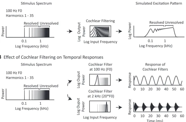
Figure 1. Effects of cochlear filtering on pitch cues. A, Spectral resolvability varies with harmonic number. Left, Power spectrum of an example periodic complex tone. Any periodic stimulus contains power at frequencies that are multiples of the F0. These frequencies are equally spaced on a linear scale, but grow closer together on a logarithmic scale. Middle, Frequency response of a bank of gammatone filters (Slaney, 1998;Ellis, 2009) intended to mimic the frequency tuning of the cochlea. Cochlear filter bandwidths are relatively constant on a logarithmic frequency scale (though they do broaden at low frequencies). Right, Simulated excitation pattern (giving the magnitude of the cochlear response as a function of frequency) for the complex tone shown at left. Cochlear filtering has the effect of smoothing the original stimulus spectrum. Low-numbered harmonics yield resolvable peaks in the excitation pattern, providing a spectral cue to pitch. High-numbered harmonics, which are closely spaced on a log scale, are poorly resolved after filtering because many harmonics fall within a single filter and thus do not provide a spectral pitch cue.

B, Temporal pitch cues in the cochlea’s output. Left, Power spectrum of a periodic complex tone. Middle, Frequency response of two example cochlear filters superimposed on the example stimulus

spectrum. Right, Response of each example filter plotted over a brief temporal interval. Both resolved and unresolved harmonics produce periodic fluctuations in the temporal response of individual cochlear filters.

A

B

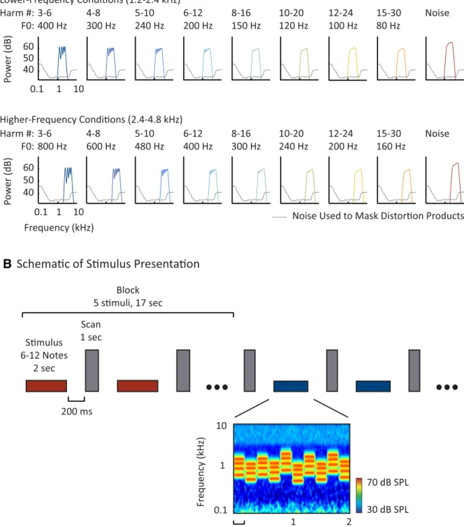
Figure 2. Study design. A, Simulated excitation patterns for example notes from each harmonic and noise condition in the parametric resolvability experiment (see Materials and Methods for details). Two frequency ranges (rows) were crossed with eight sets of harmonic numbers (columns) to yield 16 harmonic conditions. As can be seen, the excitation peaks decrease in definition with increasing harmonic number (left to right), but are not greatly affected by changes in F0 or absolute frequency that do not alter harmonic number (top to bottom). Complexes with harmonics below the eighth are often considered resolved because they are believed to produce excitation peaks and troughs separated by at least 1 dB (Micheyl et al., 2010). For each frequency range, a spectrally matched noise control was included as a nonpitch baseline (the spectrum level of the noise was increased by 5 dB relative to the harmonic conditions to equalize perceived loudness). B, Schematic of stimulus presentation. Stimuli (denoted by horizontal bars) were presented in a block design, with five stimuli from the same condition presented successively in each block (red and blue indicate different conditions). Each stimulus was 2 s in duration and included 6 –12 different notes. After each stimulus, a single scan was collected (vertical, gray bars). To minimize note-to-note adaptation, notes within a given stimulus/condition varied in their frequency and F0 within a limited range specified for that condition (such that harmonic number composition did not vary across the notes of a condition). A cochleogram for an example stimulus is shown at the bottom (plotting the magnitude of the cochlear response as a function of frequency and time, computed using a gammatone filterbank). Masking noise is visible at low and high frequencies.

Resolvability is believed to be determined by the spacing of harmonics relative to cochlear filter bandwidths, a key consequence of which is that the resolvability of a harmonic depends primarily on its number in the harmonic sequence (i.e., the ratio between its frequency and the F0) rather than on absolute frequency or absolute F0 (Figs. 1A,2A;Houtsma and Smurzinski, 1990;Carlyon and Shackleton, 1994;Shackleton and Carlyon, 1994;Plack et al., 2005). This is because auditory filter band-widths increase with the center frequency of the filter on a linear fre-quency scale and are relatively constant when plotted on a logarithmic scale (although not perfectly constant, seeGlasberg and Moore, 1990), whereas harmonics are separated by a fixed amount on a linear scale and thus grow closer together on a logarithmic scale as harmonic number increases. As a result, low-numbered harmonics, which fall under filters that are narrow relative to the harmonic spacing, produce detectable peaks in the cochlea’s excitation pattern, whereas high-numbered har-monics do not (Figs. 1A,2A). In contrast, both resolved and unresolved

harmonics produce periodic fluctuations in the temporal response of individual cochlear nerve fibers (Fig. 1B), because multiple harmonics

passed through the same frequency channel produce beating at the fre-quency of the F0.

The key piece of evidence that resolved harmonics are important for pitch perception is that complexes with only high-numbered harmonics produce a weaker pitch percept than complexes with low-numbered harmonics (Houtsma and Smurzinski, 1990;Shackleton and Carlyon, 1994). Behaviorally, this effect manifests as a sharp increase in pitch discrimination thresholds when the lowest harmonic in a complex (gen-erally the most resolved component) is higher than approximately the eighth harmonic (Bernstein and Oxenham, 2005). This “cutoff” point is relatively insensitive to the absolute frequency range or F0 of the com-plex, as can be demonstrated experimentally by fixing the stimulus fre-quency range and varying the F0 or, conversely, by fixing the F0 and varying the frequency range (Shackleton and Carlyon, 1994;Penagos et al., 2004).

General methods

Stimuli for parametric resolvability manipulation. Because controlling for

stimulus frequency content is particularly important in studying audi-tory neural responses, we presented harmonics within a fixed absolute frequency range when manipulating resolvability (Fig. 2A, each row has

the same frequency range). The resolvability of each harmonic complex was varied by changing the F0, which alters the harmonic numbers pres-ent within the fixed frequency range (Fig. 2A, harmonic numbers

in-crease from left to right). To control for effects of F0, we tested two different frequency ranges, presenting the same harmonic numbers with different F0s (Fig. 2A; top and bottom rows have the same harmonic

numbers, but different F0s and frequency ranges). Behaviorally, we ex-pected that pitch discrimination thresholds would be high (indicating poor performance) for complexes in which the lowest component was above the eighth harmonic and that this cutoff point would be similar across the two frequency ranges (Shackleton and Carlyon, 1994; Bern-stein and Oxenham, 2005). The goal of this part of the study was to test whether pitch-sensitive brain regions preferentially respond to harmon-ics that are resolved and, if so, whether they exhibit a nonlinear response cutoff as a function of harmonic number, similar to that measured behaviorally.

There were 18 conditions in this first part of the study: 16 harmonic conditions and two noise controls. Across the 16 harmonic conditions, we tested eight sets of harmonic numbers (Fig. 2A, columns) in two

different frequency ranges (Fig. 2A, rows). The noise conditions were

separately matched to the two frequency ranges used for the harmonic conditions.

Stimuli were presented in a block design with five stimuli from the same condition presented successively in each block (Fig. 2B). Each

stim-ulus lasted 2 s and was composed of several “notes” of equal duration. Notes were presented back to back with 25 ms linear ramps applied to the beginning and end of each note. The number of notes per stimulus varied (with equal probability, each stimulus had 6, 8, 10, or 12 notes) and the duration of each note was equal to the total stimulus duration (2 s) divided by the number of notes per stimulus. After each stimulus, a single

scan/volume was collected (“sparse sampling”;Hall et al., 1999). Each scan acquisition lasted 1 s, with stimuli presented during the 2.4 s interval between scans (for a total TR of 3.4 s). A fixed background noise was present throughout the 2.4 s interscan interval to mask distortion prod-ucts (see details below).

To minimize note-to-note adaptation, we varied the frequency range and F0 of notes within a condition over a 10-semitone range. The F0 and frequency range covaried such that the power at each harmonic number remained the same, ensuring that all notes within a condition would be similarly resolved (Fig. 2B, cochleogram). This was implemented by first

sampling an F0 from a uniform distribution on a log scale, then generat-ing a complex tone with a full set of harmonics, and then band-pass filtering this complex in the spectral domain to select the desired set of harmonic numbers. The filter cutoffs for the notes within a condition were thus set relative to the note harmonics. For example, the filter cutoffs for the most resolved condition were set to the third and sixth harmonic of each note’s F0 (e.g., a note with a 400 Hz F0 would have a passband of 1200 –2400 Hz and a note with 375 Hz F0 would have a passband of 1125–2250 Hz).

The 8 passbands for each frequency range corresponded to harmonics 3– 6, 4 – 8, 5–10, 6 –12, 8 –16, 10 –20, 12–24, and 15–30. For the 8 lower frequency conditions, the corresponding mean F0s were 400 Hz (for harmonics 3– 6), 300 Hz (for harmonics 4 – 8), 240 Hz (5–10), 200 Hz (6 –12), 150 Hz (8 –16), 120 Hz (10 –20), 100 Hz (12–24), and 80 Hz (15–30). These conditions spanned the same frequency range because the product of the mean F0 and the lowest/highest harmonic number of each passband was the same for all 8 conditions (e.g., 400*[3 6]⫽ 300*[4 8] ⫽ 240*[5 10] etc.). For the 8 conditions with a higher-frequency range, the corresponding F0s were an octave higher (800 Hz for harmonics 3– 6, 600 Hz for harmonics 4 – 8, etc.).

For all conditions, harmonics were added in sine phase, and the skirts of the filter sloped downward at 75 dB/octave (i.e., a linear decrease in amplitude for dB-amplitude and log-frequency scales). We chose to ma-nipulate the harmonic content of each note via filtering (as opposed to including a fixed number of equal-amplitude components) to avoid sharp spectral boundaries, which might otherwise provide a weakly re-solved pitch cue, perhaps due to lateral inhibition (Small and Daniloff, 1967;Fastl, 1980).

The two noise conditions were matched in frequency range to the harmonic conditions (with one noise condition for each of the two fre-quency ranges). For each noise note, a “reference frefre-quency” (the analog of an F0) was sampled from a uniform distribution on a log-scale and Gaussian noise was then band-pass filtered relative to this sampled ref-erence frequency. For the lower frequency noise condition, the mean reference frequency was 400 Hz and the passband was set to 3 and 6 times the reference frequency. For the high-frequency noise condition, the mean reference frequency was increased by an octave to 800 Hz.

Figure 2A shows simulated excitation patterns for a sample note from

each condition (for illustration purposes, F0s and reference frequencies are set to the mean for the condition). These excitation patterns were computed from a standard gammatone filter bank (Slaney, 1998;Ellis, 2009) designed to give an approximate representation of the degree of excitation along the basilar membrane of the cochlea. It is evident that harmonics above the eighth do not produce discernible peaks in the excitation pattern.

Harmonic notes were presented at 67 dB SPL and noise notes were presented at 72 dB SPL; the 5 dB increment was chosen based on pilot data suggesting that this increment was sufficient to equalize loudness between harmonic and noise notes. The sound level of the harmonic conditions was chosen to minimize earphone distortion (see below).

Measuring and controlling for distortion products. An important

chal-lenge when studying pitch is to control for cochlear distortion products (DPs)—frequency components introduced by nonlinearities in the co-chlea’s response to sound (Goldstein, 1967). This is particularly impor-tant for examining the effects of resolvability because distortion can introduce low-numbered harmonics not present in the original stimulus. Although an unresolved pitch stimulus might be intended to convey purely temporal pitch information, the DPs generated by an unresolved stimulus can in principle act as a resolved pitch cue. To eliminate the

potentially confounding effects of distortion, we used colored noise to energetically mask distortion products, a standard approach in both psy-chophysical and neuroimaging studies of pitch perception (Licklider, 1954;Houtsma and Smurzinski, 1990;Penagos et al., 2004;Hall and Plack, 2009).

Cochlear DPs were estimated psychophysically using the beat-cancellation technique (Goldstein, 1967; Pressnitzer and Patterson, 2001). This approach takes advantage of the fact that cochlear DPs are effectively pure tones and can therefore be cancelled using another pure tone at the same amplitude and opposite phase as the DP. The effect of cancellation is typically made more salient with the addition of a second tone designed to produce audible beating with the DP when present (i.e., not cancelled). Because the perception of beating is subtle in this para-digm, the approach requires some expertise, and thus DP amplitudes were estimated by author S.N.-H. in both ears and replicated in a few conditions by two other laboratory members. We used the maximum measured DP across the two ears of S.N.-H. as our estimate of the distor-tion spectrum. The DP amplitudes we measured for our stimuli were similar to those reported byPressnitzer and Patterson (2001)for an unresolved harmonic complex.

We found that the amplitude of cochlear DPs primarily depended on the absolute frequency of the DP (as opposed to the harmonic number of the DP relative to the primaries) and that lower-frequency DPs were almost always higher in amplitude (a pattern consistent with the results ofPressnitzer and Patterson, 2001, and likely in part explained by the fact that the cancellation tone, but not the DP, is subject to the effects of middle ear attenuation). As a conservative estimate of the distortion spectrum (e.g., the maximum cochlear DP generated at each frequency), we measured the amplitude of DPs generated at the F0 for a sample harmonic complex from every harmonic condition (with the F0 set to the mean of the condition) and used the maximum amplitude at each abso-lute frequency to set our masking noise at low frequencies.

Distortion can also arise from nonlinearities in sound system hard-ware. In particular, the MRI-compatible Sensimetrics earphones we used to present sound stimuli in the scanner have higher levels of distortion than most high-end audio devices due to the piezo-electric material used to manufacture the earphones (according to a personal communication with the manufacturers of Sensimetrics earphones). Sensimetrics ear-phones have nonetheless become popular in auditory neuroimaging be-cause (1) they are MRI-safe, (2) they provide considerable sound attenuation via screw-on earplugs (necessary because of the loud noise produced by most scan sequences), and (3) they are small enough to use with modern radio-frequency coils that fit snugly around the head (here we use a 32-channel coil). To ensure that earphone distortion did not influence our results, we presented sounds at a moderate sound level (67 dB SPL for harmonic conditions) that produced low earphone distortion, and we exhaustively measured all of the earphone DPs generated by our stimuli (details below). We then adjusted our mask-ing noise to ensure that both cochlear and earphone DPs were ener-getically masked.

Distortion product masking noise. The masking noise was designed to

be at least 10 dB above the masked threshold of any cochlear or earphone DP, i.e. the level at which the DP would have been just detectable. This relatively conservative criterion should render all DPs inaudible. To ac-complish this while maintaining a reasonable signal-to-noise ratio, we used a modified version of threshold-equalizing noise (TEN) (Moore et al., 2000) that was spectrally shaped to have greater power at frequencies with higher-amplitude DPs. The noise took into account the DP level, the auditory filter bandwidth at each frequency, and the efficiency with which a tone can be detected at each frequency. For frequencies between 400 Hz and 5 kHz, both cochlear and earphone DPs were low in ampli-tude (never exceeding 22 dB SPL) and the level of the TEN noise was set to mask pure tones below 32 dB SPL. At frequencies below 400 Hz, cochlear DPs always exceeded earphone DPs and increased in amplitude with decreasing frequency. We therefore increased the spectrum of the TEN noise at frequencies below 400 Hz by interpolating the cochlear distortion spectrum (measured psychophysically as described above) and adjusting the noise such that it was at least 10 dB above the masked

threshold of any DP. For frequencies above 5 kHz, we increased the level of the TEN noise by 6 dB to mask Sensimetrics earphone DPs, which reached a peak level of 28 dB SPL at 5.5 kHz (due to a high-frequency resonance in the earphone transfer function). This 6 dB increment was implemented with a gradual 15 dB per octave rise (from 3.8 to 5 kHz). The excitation spectrum of the masking noise can be seen inFigure 2A

(gray lines).

Earphone calibration and distortion measurements. We calibrated

stim-ulus levels using a Svantek 979 sound meter attached to a G.R.A.S. mi-crophone with an ear and cheek simulator (Type 43-AG). The transfer function of the earphones was measured using white noise and was in-verted to present sounds at the desired level. Distortion measurements were made with the same system. For each harmonic condition in the experiment, we measured the distortion spectrum for 11 different F0s spaced 1 semitone apart (to span the 10-semitone F0 range used for each condition). For each note, DPs were detected and measured by comput-ing the power spectrum of the waveform recorded by the sound meter and comparing the measured power at each harmonic to the expected power based on the input signal and the transfer function of the ear-phones. Harmonics that exceeded the expected level by 5 dB SPL were considered DPs. Repeating this procedure across all notes and conditions produced a large collection of DPs, each with a specific frequency and power. At the stimulus levels used in our experiments, the levels of ear-phone distortion were modest. Below 5 kHz, the maximum DP measured occurred at 1.2 kHz and had an amplitude of 22 dB SPL. Above 5 kHz, the maximum DP measured was 28 dB SPL and occurred at 5.5 kHz. We found that higher stimulus levels produced substantially higher ear-phone distortion for stimuli with a peaked waveform, such as the unre-solved pitch stimuli used in this study, and such levels were avoided for this reason.

Tonotopy stimuli. We measured tonotopy using pure tones presented

in one of six different frequency ranges spanning a six-octave range, similar to the approach used byHumphries et al. (2010). The six fre-quency ranges were presented in a block design using the same approach as that for the harmonic and noise stimuli. For each note, tones were sampled from a uniform distribution on a log scale with a 10-semitone range. The mean of the sampling distribution determined the frequency range of each condition and was set to 0.2, 0.4, 0.8, 1.6, 3.2, and 6.4 kHz. There were more notes per stimulus for the pure tone stimuli than for the harmonic and noise stimuli (with equal probability, a stimulus contained 16, 20, 24, or 30 notes), because in pilot data we found that frequency-selective regions responded most to fast presentation rates. The sound level of the pure tones was set to equate their perceived loudness in terms of sones (8 sones, 72 dB SPL at 1 kHz), using a standard loudness model (Glasberg and Moore, 2006).

Stimuli for efficient pitch localizer. Based on the results of our

paramet-ric resolvability manipulation, we designed a simplified set of pitch and noise stimuli to localize pitch-responsive brain regions efficiently in each subject while minimizing earphone distortion. Specifically, our pitch localizer consisted of a resolved pitch condition contrasted with a frequency-matched noise control. We chose to use resolved harmonics exclusively because they produced a much higher response in all cortical pitch regions than did unresolved harmonics. Moreover, the use of a single resolved condition allowed us to design a harmonic stimulus that produced very low Sensimetrics earphone distortion even at higher sound levels (achieved by minimizing the peak factor of the waveform and by presenting sounds in a frequency range with low distortion). Given the increasing popularity of Sensimetrics earphones, this localizer may provide a useful tool for identifying pitch-sensitive regions in future research (and can be downloaded from our website). To assess the effec-tiveness of this localizer, we used it to identify pitch-sensitive voxels in each subject and compared the results with those obtained using the resolved harmonic and noise stimuli from the main experiment. The results of this analysis are described at the end of Part 2 in the Results. We also used the localizer to identify pitch-sensitive voxels in the four sub-jects who participated in a follow-up scan.

Harmonic and noise notes for the localizer stimuli were generated using the approach described previously for our parametric experimental

stimuli and were also presented in a block design. The mean F0 of the harmonic localizer conditions was 333 Hz and the passband included harmonics 3 through 6 (equivalent to the most resolved condition from the parametric manipulation in Part 1 of this study). Harmonic notes were presented at 75 dB SPL and noise notes were presented at 80 dB SPL (instead of the lower levels of 67 and 72 dB SPL used in the parametrically varied stimuli; we found in pilot experiments that higher presentation levels tend to produce higher BOLD responses). Harmonics were added in negative Schroeder phase (Schroeder, 1970) to further reduce ear-phone DPs, which are largest for stimuli with a high peak factor (percep-tually, phase manipulations have very little effect for a resolved pitch stimulus because the individual harmonics are filtered into distinct re-gions of the cochlea). Cochlear DPs at the F0 and second harmonic were measured for complexes with three different F0s (249, 333, and 445 Hz, which corresponded to the lowest, highest, and mean F0 of the har-monic notes), and modified TEN noise was used to render DPs inau-dible. The spectrum of the TEN noise was set to ensure that DPs were at least 15 dB below their masked threshold (an even more conserva-tive criterion than that used in Part 1 of the study). Specifically, below 890 Hz (the maximum possible frequency of the second harmonic), the level of the TEN noise was set to mask DPs up to 40 dB SPL. Above 890 Hz, the noise level was set to mask DPs up to 30 dB SPL. The 10 dB decrement above 890 Hz was implemented with a gradual 15 dB per octave fall-off from 890 Hz to 1.4 kHz. Earphone DPs never exceeded 15 dB SPL for these stimuli.

Participants. Twelve individuals participated in the fMRI study (4

male, 8 female, all right-handed, ages 21–28 years, mean age 24 years). Eight individuals from the fMRI study also participated in a behavioral experiment designed to measure pitch discrimination thresholds for the same stimuli. To obtain robust tonotopy and pitch maps in a subset of individual subjects, we rescanned four of the 12 subjects in a follow-up session.

Subjects were non-musicians (with no formal training in the 5 years preceding the scan), native English speakers, and had self-reported nor-mal hearing. Pure-Tone detection thresholds were measured in all participants for frequencies between 125 Hz and 8 kHz. Across all fre-quencies tested, 7 subjects had a maximum threshold at or below 20 dB HL, 3 subjects had a maximum threshold of 25 dB HL, and 1 subject had a maximum threshold of 30 dB HL. One subject had notable high-frequency hearing loss in the right ear (with thresholds of 70 dB HL and higher for frequencies 6 kHz and above; left ear thresholds were⬍20 dB HL at all frequencies and right ear thresholds were at or below 30 dB for all other frequencies). Neural data from this subject was included in our fMRI analyses, but the inclusion or exclusion of their data did not qual-itatively alter the results. This subject did not participate in the behavioral experiment. Two additional subjects (not included in the 12 described above) were excluded from the study either because not enough data were collected (due to a problem with the scanner) or because the subject reported being fatigued throughout the experiment. In the latter case, the decision to exclude the subject was made before analyzing their data to avoid any potential bias. The study was approved by the Committee On the Use of Humans as Experimental Subjects (COUHES) at the Massa-chusetts Institute of Technology (MIT), and all participants gave in-formed consent.

Procedure. Scanning sessions lasted 2 h and were composed of multiple

functional “runs,” each lasting 6 –7 min. Two types of runs were used in the study. The first type (“resolvability runs”) included all of the har-monic and noise stimuli for our parametric resolvability manipulation (i.e., all of the conditions illustrated inFig. 2A). The second type

(“tono-topy runs”) included all of the tono(“tono-topy stimuli as well as the pitch and noise conditions for the efficient pitch localizer. Runs with excessive head motion or in which subjects were overly fatigued were discarded before analysis. Not including discarded runs, each subject completed 7– 8 re-solvability runs and 3 tonotopy runs. The 4 subjects who participated in a second scanning session completed 10 –12 tonotopy runs (these extra 7–9 runs were not included in group analyses across all 12 subjects to avoid biasing the results). Excessive motion was defined as at least 20 time points whose average deviation (Jenkinson, 1999) from the previous time point exceeded 0.5 mm. Fatigue was obvious due a sudden drop in

re-sponse rates on the repetition-detection task (e.g., a drop from a 90% response rate to a response rate⬍50%, see below). Across all 12 subjects, a total of two runs were discarded due to head motion and two runs were discarded due to fatigue. In addition, data from a second scanning ses-sion with a fifth subject was excluded (before being analyzed) because response rates were very low in approximately half of the runs.

Each resolvability run included one stimulus block for each of the 18 conditions shown inFigure 2A (each block lasting 17 s) as well as four

“null” blocks with no sound stimulation (also 17 s) to provide a baseline (each run included 114 scans and was 385 s in total duration). Each tonotopy run included two stimulus blocks for each of the six pure-tone conditions, four stimulus blocks for each of the harmonic and noise conditions from the pitch localizer, and five null blocks (129 scans, 436 s). The order of stimulus and null blocks was counterbalanced across runs and subjects such that, on average, each condition was approxi-mately equally likely to occur at each point in the run and each condition was preceded equally often by every other condition in the experiment. After each run, subjects were given a short break (⬃30 s).

To help subjects attend equally to all of the stimuli, subjects performed a “1-back” repetition detection task (responding whenever successive 2 s stimuli were identical) across stimuli in each block for both resolvability and tonotopy runs. Each block included four unique stimuli and one back-to-back repetition (five stimuli per block). Each of the unique stim-uli had a different number of notes. Stimstim-uli were never repeated across blocks. Performance on the 1-back task was high for all of the harmonic and noise conditions in the experiment (hit rates between 84% and 93% and false alarm rates between 0% and 2%). Hit rates for the pure-tone conditions varied from 71% (6.4 kHz condition) to 89% (1.6 kHz condition).

Data acquisition. All data were collected using a 3T Siemens Trio

scan-ner with a 32-channel head coil (at the Athinoula A. Martinos Imaging Center of the McGovern Institute for Brain Research at MIT). T1-weighted structural images were collected for each subject (1 mm isotro-pic voxels). Each functional volume (e.g., a single whole-brain acquisition) comprised 15 slices oriented parallel to the superior tempo-ral plane and covering the portion of the tempotempo-ral lobe superior to and including the superior temporal sulcus (3.4 s TR, 1 s TA, 30 ms TE, 90 degree flip angle; the first 5 volumes of each run were discarded to allow for T1 equilibration). Each slice was 4 mm thick and had an in-plane resolution of 2.1 mm⫻ 2.1 mm (96 ⫻ 96 matrix, 0.4 mm slice gap).

Preprocessing and regression analyses. Preprocessing and regression

analyses were performed using FSL 4.1.3 and the FMRIB software librar-ies (Analysis Group, FMRIB, Oxford;Smith et al., 2004). Functional images were motion corrected, spatially smoothed with a 3 mm FWHM kernel, and high-pass filtered (250 s cutoff). Each run was fit with a general linear model (GLM) in the native functional space. The GLM included a separate regressor for each stimulus condition (modeled with a gamma hemodynamic response function) and six motion regressors (three rotations and three translations). Statistical maps from this within-run analysis were then registered to the anatomical volume using FLIRT (Jenkinson and Smith, 2001) followed by BBRegister (Greve and Fischl, 2009).

Surface-based analyses. For anatomical and tonotopy analyses, these

within-run maps were resampled to the cortical surface, as estimated by Freesurfer (Fischl et al., 1999), and combined across runs within subjects using a fixed effects analysis. For simplicity, we use the term “voxel” in describing all of our analyses rather than switching to the slightly more accurate term “vertex” when discussing surface-based analyses (vertices refer to a 2D point on the cortical surface).

Analyses for Part 1: Cortical responses to resolved and

unresolved harmonics

ROI analyses of cortical pitch responses. To test the response of

pitch-sensitive brain regions, we first identified voxels in the superior temporal plane of each subject that responded more to all 16 harmonic conditions compared with the two frequency-matched noise conditions (the localize phase) and then measured the response of these voxels in independent (left-out) data to all 18 conditions (the test phase;Fig. 3A, B,D).

resolvabil-ity effects because it included both resolved and unresolved harmonics. We considered only voxels that fell within an anatomical constraint re-gion encompassing the superior temporal plane. This constraint rere-gion spanned HG, the planum temporale, and the planum polare and was defined as the combination of the 5 ROIs used in the anatomical analyses (Fig. 4A). We chose the superior temporal plane as a constraint region

because almost all prior reports of pitch responses have focused on this region and because, in practice, we rarely observed consistent pitch re-sponses outside of the superior temporal plane.

We implemented this localize-and-test procedure using a simple leave-one-out design performed across runs, similar to the approach typically used in classification paradigms such as multivoxel pattern analysis (Norman et al., 2006). With 3 runs, for example, there would be 3 localize/test pairs: localize with runs 2 and 3 and test with run 1, localize with runs 1 and 3 and test with run 2, and localize with runs 1 and 2 and test with run 3. For each localize-test pair, we identified pitch-sensitive voxels using data from every run except the test run and we then measured the mean response of these localized voxels to all 18 harmonic and noise conditions in the test run. Each run therefore provided an unbiased sample of the response to every condi-tion and we averaged responses across runs to derive an estimate of the response to each condition in each subject.

For the localize phase, we computed subject-specific significance maps using a fixed-effects analysis across all runs except the test run and se-lected the 10% of voxels with the most significant response within the anatomical constraint region (due to variation in brain size, the total volume of these voxels ranged from 1.1 to 1.6 cm3_{across subjects). We} chose to use a fixed percentage of voxels instead of a fixed significance threshold (e.g., p⬍ 0.001) because differences in significance values across subjects are often driven by generic differences in signal-to-noise that are unrelated to neural activity (such as amount of motion). In the test phase, we then measured the response of these voxels in independent data.

For the test phase, we measured the mean response time course for each condition by averaging the signal from each block from that condi-tion. Time courses were then converted to percent signal change by sub-tracting and dividing by the mean time course for the null blocks (pointwise, for each time point of the block). The mean response to each condition was computed by averaging the response of the second through fifth time points after the onset of each block. Response time courses are shown inFigure 3A and the gray area indicates the time points

included in the average response for each condition.

Behavioral pitch discrimination experiment. To assess the perceptual

effects of our resolvability manipulation, we measured pitch discrimina-tion thresholds for all of the harmonic condidiscrimina-tions in the study for a subset of eight subjects from the imaging experiment (Fig. 3C,E). Subjects were

asked to judge which of two sequentially presented notes was higher in pitch. We used an adaptive procedure (3-up, 1-down) to estimate the F0 difference needed to achieve 79% accuracy (Levitt, 1971). Subjects com-pleted between one and three adaptive sequences for each of the 16 harmonic conditions tested in the imaging experiment (five subjects completed two sequences, two subjects completed three sequences, and one subject completed a single sequence). In each sequence, we measured 12 reversals and the threshold for a given subject and condition was defined as the geometric mean of the last eight reversal points of each sequence. The frequency difference at the start of the sequence was set to 40% and this difference was updated by a factor of 1.414 (square root of 2) for the first 4 reversals and by a factor of 1.189 (fourth root of 2) for the last 8 reversals.

The “notes” used as stimuli in the behavioral experiment were de-signed to be as similar as possible to the notes used in the imaging exper-iments, subject to the constraints of a discrimination experiment. To encourage subjects to rely on pitch cues as opposed to overall frequency cues, each pair of notes on a given trial was filtered with the same filter, such that the frequency range was constant across the notes of a single trial. This was partially distinct from the imaging experiment, in which each note had a unique filter defined relative to its F0, but was necessary to isolate F0 discrimination behaviorally. The filter cutoffs for a note pair were set relative to the center frequency (geometric mean) of the F0s for

the two notes using the same procedure as that for the imaging experi-ment. Center frequencies were varied across trials (uniformly sampled from⫾10% of the mean F0 for that condition) to encourage subjects to compare notes within a trial instead of making judgments based on the distribution of frequencies across trials (e.g., by judging whether a note is higher or lower in frequency than the notes in previous trials). The mean F0 of each condition was the same as that used in the imaging experi-ment. Each note was 333 ms in duration and pairs of notes were separated by a 333 ms interstimulus interval. We used the same MRI-compatible earphones to measure behavioral thresholds and the same colored noise to mask cochlear and earphone distortion. Masking noise was gated on 200 ms before the onset of the first note and was gated off 200 ms after the offset of the second note (25 ms linear ramps). Conditions with the same frequency range were grouped into sections and participants were en-couraged to take a break after each section. The order of low- and high-frequency sections was counterbalanced across subjects and the order of conditions within a section was randomized.

Analyses for Part 2: Anatomical location of cortical pitch responses

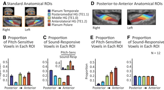
pitch-sensitive brain regions, we divided the superior temporal plane into five nonoverlapping anatomical ROIs (based on prior literature, as detailed below;Fig. 4A) and measured the proportion of pitch-sensitive voxels

that fell within each region.

We again identified pitch-sensitive voxels as those responding prefer-entially to harmonic tones compared with noise (the top 10% of voxels in the superior temporal plane with the most significant response to this contrast) and then measured the number of pitch-sensitive voxels that fell within each subregion of the superior temporal plane (Fig. 4B).

Be-cause the 5 anatomical ROIs subdivided our superior temporal plane ROI, this analysis resulted in a 5-bin histogram, which we normalized to sum to 1 for each subject. As a baseline, we also measured the proportion of sound-responsive voxels that fell within each region (Fig. 4C).

Sound-responsive voxels were defined by contrasting all 18 stimulus conditions with silence (voxel threshold of p⬍ 0.001). To compare the anatomical distribution of pitch and sound responses directly, we also computed the proportion of sound-responsive voxels in each region that exhibited a pitch response (Fig. 4C, inset).

The five ROIs corresponded to posteromedial HG (TE1.1), middle HG (TE1.0), anterolateral HG (TE1.2), planum temporale (posterior to HG), and planum polare (anterior to HG). The HG ROIs are based on human postmortem histology (Morosan et al., 2001) and the temporal plane ROIs (planum polare and planum temporale) are based on human mac-roscopic anatomy (distributed in FSL as the Harvard Cortical Atlas; Desi-kan et al., 2006). To achieve better surface-based alignment and to facilitate visualization, the ROIs were resampled to the cortical surface of the MNI305 template brain (Fig. 4A).

The distribution of pitch responses across these five ROIs suggested that pitch responses might be more concentrated in anterior regions of auditory cortex. To test this idea directly, we performed the same analysis using a set of five novel ROIs that were designed to run along the posterior-to-anterior axis of the superior temporal plane, demar-cated so as to each include an equal number of sound-responsive voxels (Figs. 4D–F ). We created these five ROIs by: (1) flattening the

cortical surface (Fischl et al., 1999) to create a 2D representation of the superior temporal plane, (2) drawing a line on the flattened sur-face that ran along the posterior-to-anterior axis of HG, (3) sorting voxels based on their projected location on this line, and (4) grouping voxels into five regions such that, on average, each region would have an equal number of sound-responsive voxels. This final step was im-plemented by computing a probability map expressing the likelihood that a given voxel would be classified as sound-responsive and then constraining the sum of this probability map to be the same for each region. The main effect of this constraint was to enlarge the size of the most anterior ROI to account for the fact that auditory responses occur less frequently in the most anterior portions of the superior temporal plane. The anatomical ROIs used in the study can be down-loaded from our website.

Anatomical distribution of resolvability effects across auditory cortex. To

test whether effects of resolvability are present throughout auditory cor-tex, we performed the localize-and-test ROI analysis within the five posterior-to-anterior ROIs from the previous analysis (Fig. 5). For a given ROI, we identified the 10% of voxels (within that ROI) in each subject with the most significant response preference for harmonic tones compared with noise and measured their response to each condition in independent data.

Analyses for Part 3: The tonotopic location of pitch-sensitive

brain regions

The results from Parts 1 and 2 of our study suggested that pitch-sensitive regions are localized to the anterior half of auditory cortex and that pitch responses throughout auditory cortex are driven predominantly by the presence of resolved harmonics. To further clarify the anatomical orga-nization of pitch responses, we computed whole-brain maps of pitch responses and tonotopy. Because these analyses were qualitative, we quantified and validated the main results from these analyses by per-forming within-subject ROI analyses.

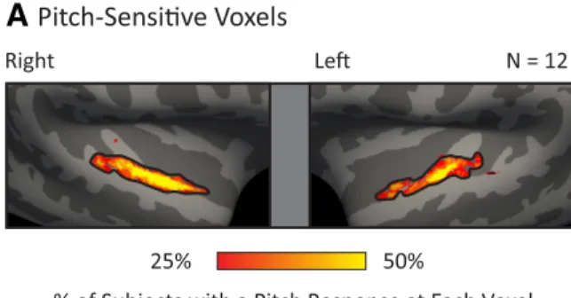
Whole-brain map of pitch responses. For comparison with tonotopy

maps, we computed a whole-brain summary figure indicating the proportion of subjects with a pitch response at each point on the cortical surface (Fig. 6A). We focused on pitch responses to

condi-tions with resolved harmonics (defined as having harmonics below the eighth component) because we found in Part 1 that resolved pitch stimuli produced larger pitch responses throughout auditory cortex and thus provide the most robust measure of pitch sensitivity. Pitch-sensitive voxels were defined in each subject as the 10% of voxels in the superior temporal plane that responded most significantly to tones with resolved harmonics compared with noise. For each voxel, we then counted the proportion of subjects in which that voxel was identified as pitch-sensitive. To help account for the lack of exact overlap across subjects in the location of functional responses, anal-yses were performed on lightly smoothed significance maps (3 mm FWHM kernel on the surface; without this smoothing, group maps appear artificially pixelated).

Whole-brain map of best frequency. For each subject, we computed

best-frequency maps by assigning each voxel in the superior temporal plane to the pure-tone condition that produced the maximum response, as estimated by the␤-weights from the regression analysis (Fig. 6B).

Because not all voxels in a given subject were modulated by frequency, we masked this best-frequency map using the results of a one-way, fixed-effects ANOVA across the six pure-tone conditions ( p⬍ 0.05). Group tonotopy maps were computing by smoothing (3 mm FWHM) and av-eraging the individual-subject maps, masking out those voxels that did not exhibit a significant frequency response in at least three subjects (as determined by the one-way ANOVA).

ROI analysis of low- and high-frequency voxels. To further quantify the

relationship between pitch responses and frequency tuning, we measured the response of low- and high-frequency-selective voxels to the harmonic and noise conditions (Fig. 6C). Voxels selective for low frequencies were

identified in each subject individually as the 10% of voxels with the most significant response preference for low versus high frequencies (using responses to the tonotopy stimuli: 0.2⫹ 0.4 ⫹ 0.8 kHz ⬎ 1.6 ⫹ 3.2 ⫹ 6.4 kHz). High-frequency voxels were defined in the same way using the reverse contrast (1.6⫹ 3.2 ⫹ 6.4 kHz ⬎ 0.2 ⫹ 0.4 ⫹ 0.8 kHz). We then measured the average response of these voxels to the resolved harmonic and noise conditions used to identify pitch responses in the whole-brain analysis.

Whole-brain map of frequency selectivity. To estimate the distribution

of (locally consistent) frequency selectivity across the cortex, we also computed maps plotting the degree of variation in the response of each voxel to the six pure-tone conditions (Fig. 6D). This was quantified as the

standard deviation in the response of each voxel to the six pure-tone conditions (estimated from regression␤-weights), divided by the mean response across all six conditions. Because such normalized measures become unstable for voxels with a small mean response (due to the small denominator), we excluded voxels that did not exhibit a significant mean response to the six pure-tone conditions relative to silence ( p⬍ 0.001)

and truncated negative responses to zero. Frequency-selectivity maps were computed for each subject, smoothed (3 mm FWHM), and aver-aged across subjects. Voxels that did not exhibit a significant sound re-sponse in at least three subjects were again excluded.

Statistical comparison of pitch responses and frequency selectivity. To

further test the relationship between pitch responses and frequency se-lectivity, we measured the frequency selectivity of pitch-sensitive voxels as a function of their posterior-to-anterior position (Fig. 6E). As in the

whole-brain analysis, pitch-sensitive voxels were identified as the 10% of voxels in each subject with the most significant response preference for resolved harmonics compared with noise. Frequency selectivity was computed for each pitch-sensitive voxel in each subject individually and was defined as the standard deviation of the response across the six pure-tone conditions divided by the mean. We then grouped voxels into 10 bins (each containing 10% of all pitch-sensitive voxels) based on their posterior-to-anterior position in that subject and averaged selectivity measures within each bin.

Maps of pitch and tonotopy within individual subjects. To demonstrate

that the effects we observed at the group level are present in individual subjects, we also present individual subject maps of pitch responses, tonotopy, and frequency selectivity for four subjects who completed an extra scanning session to increase the reliability of their tonotopic maps (Fig. 7). Pitch maps were computed by contrasting responses to resolved harmonics with noise, using data from the “efficient pitch localizer” described earlier (whole-brain maps plot the significance of this con-trast). Maps of best-frequency and frequency selectivity were computed using the same approach as the group analyses, except that there was no additional smoothing on the surface and we used a stricter criterion for defining voxels as frequency-selective when computing best-frequency maps ( p⬍ 0.001). We were able to use a stricter threshold because we had three to four times as much tonotopy data within each subject.

Control experiment: Are resolvability effects dependent on

frequency variation?

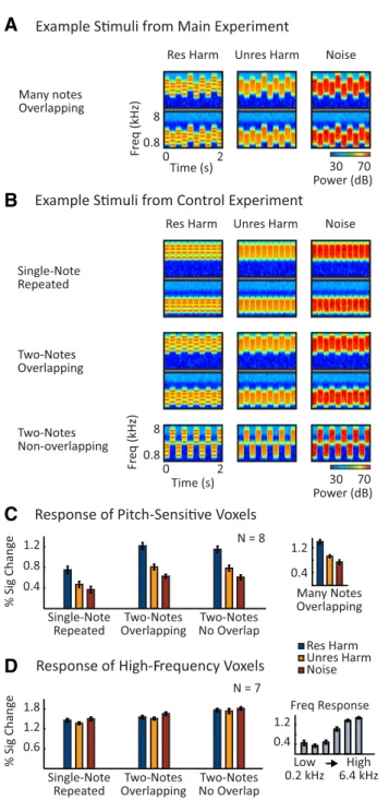
One notable feature of our main experiment was that the stimuli varied in pitch and frequency (Figs. 2B,8A). We made this design choice

be-cause in pilot experiments we repeatedly found that this variation en-hanced the cortical response and thus improves statistical power. However, it is conceivable that frequency/pitch variation could bias cor-tical responses in favor of resolved harmonics, because notes with sparser spectral representations (e.g., on the cochlea) will tend to overlap less with each other. Less note-to-note spectral overlap for resolved stimuli could reduce the effects of frequency adaptation and inflate responses to resolved harmonics relative to stimuli without resolved spectral peaks for reasons potentially unrelated to their role in pitch perception.

To rule out the possibility that resolvability effects are merely a by-product of note-to-note frequency/pitch variation, we tested whether neural resolvability effects persist for stimuli with a single, repeated note (Fig. 8B, top row). We also measured responses to stimuli with two

alternating notes and manipulated the spectral overlap between notes directly (Fig. 8B, bottom two rows). This allowed us to test whether

differences in note-to-note spectral overlap have any significant effect on the response to resolved and unresolved harmonics. In addition to con-trolling for frequency adaptation, these experiments help to link our findings more directly with those of prior studies of pitch responses, which have primarily used stimuli with repeated notes (Patterson et al., 2002;Hall and Plack, 2009).

The experiment had a 3⫻ 3 factorial design, illustrated inFigure 8B.

Each stimulus was composed of either (1) a single, repeated note, (2) two alternating notes designed to minimize spectral overlap in the resolved condition while maximizing overlap in the unresolved condition (two-notes overlapping), or (3) two alternating (two-notes with nonoverlapping frequency ranges (two-notes nonoverlapping). This manipulation was fully crossed with a resolvability/pitch manipulation: each note was ei-ther a resolved harmonic complex (harmonics 3– 6), an unresolved har-monic complex (harhar-monics 15–30), or frequency-matched noise.

All nine conditions were designed to span a similar frequency range as the stimuli in the main experiment. For the two-note stimuli with non-overlapping frequency ranges, the lower-frequency note spanned 1.2–2.4

kHz and the higher-frequency note spanned 2.88 –5.76 kHz, resulting in a 20% spectral gap between the notes (e.g., [2.88 –2.4]/2.4⫽ 0.2). For resolved complexes, the F0s of the low- and high-frequency notes were 400 and 960 Hz, respectively; for unresolved complexes, the F0s were 80 and 192 Hz, respectively. These same notes were used for the single-note condition, but each note was presented in a separate stimulus.

For the two-note conditions with overlapping frequency ranges, there was a low-frequency and a high-frequency stimulus, each with two alter-nating notes (Fig. 8B). The notes of each stimulus were separated by 2.49

semitones, an amount that minimized spectral overlap between resolved frequency components (2.49 semitones is half of the log distance between the first two resolved frequency components of the notes). The frequency range and F0s of the frequency stimuli straddled the lower-frequency notes of the nonoverlapping and single-note conditions on a log-scale (F0s and frequency ranges were 1.25 semitones above and below those used for the nonoverlapping stimuli). Similarly, the frequency and F0s of the higher-frequency stimuli straddled the higher-frequency notes of the nonoverlapping and single-note stimuli. For 4 of the 8 subjects scanned, the higher-frequency stimuli had a frequency range and F0 that was 7% lower than intended due to a technical error. This discrepancy had no obvious effect on the data, and we averaged responses across all eight subjects.

To enable the identification of pitch-sensitive voxels using the localizer contrast from our main experiment, we also presented the resolved (har-monics 3– 6), unresolved (har(har-monics 15–30), and noise stimuli from that experiment. We also included tonotopy stimuli, which allowed us to test whether frequency-selective regions (which might be expected to show the largest effects of frequency adaptation) are sensitive to differences in spectral overlap between resolved and unresolved harmonics.

Participants. Eight individuals participated in the control experiment

(3 male, 5 female, 7 right-handed, 1 left-handed, age 19 –28 years, mean age 24 years). All subjects had self-reported normal hearing and were non-musicians (7 subjects had no formal training in the 5 years preced-ing the scan; 1 subject had taken music classes 3 years before the scan). Subjects had normal hearing thresholds (⬍25 dB HL) at all tested fre-quencies (125 Hz to 8 kHz). One of the eight subjects was also a partici-pant in the main experiment. Three additional subjects (not included in the eight described above) were excluded because of low temporal signal-to-noise (tSNR) caused by excessive head motion (two before analysis, and one after). tSNR is a standard measure of signal quality in fMRI analyses (Triantafyllou et al., 2005) and was calculated for each voxel as the mean of the BOLD signal across time divided by the standard devia-tion. All of the excluded subjects had substantially lower tSNR in the superior temporal plane than nonexcluded subjects (mean tSNR of ex-cluded subjects: 54.5, 58.2, 59.0; mean tSNR for nonexex-cluded subjects: 70.4, 71.7, 78.2, 80.3, 81.2, 81.8, 83.7, 92.7). A higher percentage of sub-jects were excluded compared with the main experiment because we used a quieter scanning sequence (described below) that we found to be more sensitive to motion (possibly because of longer-than-normal echo times).

Procedure. The procedure was similar to the main experiment. There

were two types of runs: “experimental” runs and “localizer” runs. The nine conditions shown inFigure 8B were scanned in the experimental

runs. The harmonic and noise stimuli from the main experiment (used to identify pitch-sensitive regions) were scanned in the localizer runs, as were the tonotopy stimuli.

For the experimental runs, we used a quieter scanning sequence with very little acoustic power at the frequencies of the experimental stimuli (Schmitter et al., 2008;Peelle et al., 2010) to avoid any scanner-induced frequency adaptation. This quieter sequence had a single acoustic reso-nance at 516 Hz and an overall level of 75– 80 dB SPL (measured using an MRI-compatible microphone), which was further attenuated by screw-on earplugs attached to the Sensimetrics earphones. For the local-izer runs, we used the same echoplanar sequence as the main experiment to ensure that our localizer contrasts identified the same regions. We did not use the quiet sequence in the main experiment because it produces a lower-quality MR signal (lower spatial resolution and slower acquisition times for the same spatial coverage), making it difficult to test a large number of conditions.

Each subject completed 10 –12 experimental runs and 4 – 6 localizer runs. Each experimental run consisted of nine stimulus blocks, one for each condition, and three blocks of silence. Each block was 19.5 s in duration and included 5 scan acquisitions spaced 3.9 s apart. During stimulus blocks, a 2 s stimulus was presented during a 2.4 s gap between scan acquisitions. Within a block, stimuli were always composed of the same notes, but the number and duration of the notes varied in the same way as in the main experiment (each stimulus had 6, 8, 10, or 12 notes; example stimuli shown inFig. 8B have 10 notes per stimulus). The order

of stimulus and null blocks was counterbalanced across runs and subjects in the same way as the main experiment. Each localizer run consisted of 12 stimulus blocks (one for each of the six tonotopy conditions and two for each resolved, unresolved, and noise condition) and three null blocks. The design of the localizer blocks was the same as the main experiment. For both localizer and experimental runs, subjects performed a 1-back task. Scans lasted⬃2 h as in the main experiment.

Data acquisition. With the exception of the quiet scanning sequence,

all of the acquisition parameters were the same as the main experiment. For the quiet scanning sequence, each functional volume comprised 18 slices designed to cover the portion of the temporal lobe superior to and including the superior temporal sulcus (3.9 s TR, 1.5 s TA, 45 ms TE, 90 degree flip angle; the first 4 volumes of each run were discarded to allow for T1 equilibration). Voxels were 3 mm isotropic (64⫻ 64 matrix, 0.6 mm slice gap).

Analysis. We defined pitch-sensitive voxels as the 10% of voxels in the

anterior superior temporal plane with the most significant response pref-erence for resolved harmonics compared with noise (using stimuli from the localizer runs). In contrast to the main experiment, pitch responses were constrained to the anterior half of the superior temporal plane (defined as the three most anterior ROIs from the posterior-to-anterior analysis) because we found in the main experiment that the large of majority of pitch responses (89%) were located within this region. We also separately measured responses from pitch-sensitive voxels in the middle ROI from the posterior-to-anterior analysis (the most posterior ROI with a substantial number of pitch responses) and the most anterior ROI (pitch-sensitive voxels were again defined as 10% of voxels with the most significant response preference for resolved harmonics compared with noise in each region). This latter analysis was designed to test whether more anterior pitch regions show a larger response preference for stimuli with frequency variation, as suggested by prior studies ( Pat-terson et al., 2002;Warren and Griffiths, 2003;Puschmann et al., 2010). To test this possibility, we measured the relative difference in response in each ROI to the two-note and one-note conditions using a standard selectivity measure ([two-note⫺ one-note]/[two-note ⫹ one-note]) and then compared this selectivity measure across the two ROIs.

For the tonotopy analyses, we focused on regions preferring high fre-quencies because they are distinct from pitch-sensitive regions (as dem-onstrated in the main experiment) and because our stimuli spanned a relatively high-frequency range (above 1 kHz). High-frequency voxels were defined as the 10% of voxels in the superior temporal plane with the most significant response preference for high (1.6, 3.2, 6.4 kHz) versus low (0.2, 0.4 0.8 kHz) frequencies. One of the eight subjects was excluded from the tonotopy analysis because of a lack of replicable high-frequency preferring voxels in left-out test data.

Results

Part 1: Cortical responses to resolved and

unresolved harmonics

To assess the response of pitch-sensitive brain regions to spectral

and temporal cues, we first identified voxels in each subject that

respond more to harmonic complex tones than noise regardless

of resolvability (by selecting the 10% of voxels from anywhere in

the superior temporal plane with the most significant response to

this contrast). We then measured the response of these voxels to

each harmonic and noise condition in independent data.

Figure

3

A plots the average time course across these voxels for each

harmonic and noise condition, collapsing across the two

fre-quency ranges tested, and

Figure 3

B shows the response averaged

across time (shaded region in

Fig. 3

A indicates time points

in-cluded in the average).

Pitch-sensitive voxels responded approximately twice as

strongly to harmonic tones as to noise when low-numbered,

re-solved harmonics were present in the complex. In contrast, these

same brain regions responded much less to tones with only

high-numbered, unresolved harmonics, which are thought to lack

spectral pitch cues (

Figs. 1

A,

2

A). This difference resulted in a

highly significant main effect of harmonic number (F

⫽

14.93, p

⬍ 0.001) in an ANOVA on responses to harmonic

con-ditions averaged across the two frequency ranges. These results

are consistent with those of

Penagos et al. (2004)

and suggest that

spectral pitch cues are the primary driver of cortical pitch

re-sponses. Responses to unresolved harmonics were nonetheless

significantly higher than to noise, even for the most poorly

re-solved pitch stimulus we used (harmonics 15–30, t

⫽ 2.80, p ⬍

0.05), which is consistent with some role for temporal pitch cues

(

Patterson et al., 2002

).

The overall response pattern across the eight harmonic

con-ditions was strongly correlated with pitch discrimination

thresh-olds measured behaviorally for the same stimuli (r

⫽ 0.96 across

the eight stimuli;

Fig. 3

C). Neural responses were high and

dis-crimination thresholds low (indicating good performance) for

complexes for which the lowest (most resolved) component was

below the eighth harmonic. Above this “cutoff,” neural responses

and behavioral performance declined monotonically. This

find-ing suggests that spectral pitch cues may be important in drivfind-ing

cortical pitch responses in a way that mirrors, and perhaps

un-derlies, their influence on perception.

Figure 3

D plots the

re-sponse of these same brain regions separately for the two stimulus

frequency ranges we used. The response to each harmonic

con-dition is plotted relative to its frequency-matched noise control

to isolate potentially pitch-specific components of the response.

For both frequency ranges, we observed high responses (relative

to noise) for tones for which the lowest component was below the

eighth harmonic and low responses for tones with exclusively

high-numbered components (above the 10th harmonic).

Behav-ioral discrimination thresholds were also similar across the two

spectral regions (

Fig. 3

E), consistent with many prior studies

(

Shackleton and Carlyon, 1994

;

Bernstein and Oxenham, 2005

),

and were again well correlated with the neural response (r

⫽ 0.95

and 0.94 for the low- and high-frequency conditions,

respec-C

D

E

A

B

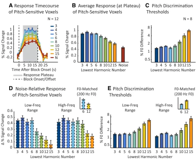
Figure 3. Response of pitch-sensitive voxels to resolved and unresolved harmonics with corresponding behavioral discrimination thresholds. A, The signal-averaged time course of pitch-sensitive voxels to each harmonic and noise condition collapsing across the two frequency ranges tested. The numeric labels for each harmonic condition denote the number of the lowest harmonic of the notes for that condition (seeFig. 2A for reference). The average time course for each condition contained a response plateau (gray area) extending from⬃5 s after the block onset (dashed vertical

line) through the duration of the stimulus block. Pitch-sensitive voxels were identified in each individual subject by contrasting all harmonic conditions with the noise conditions. B, Mean response to each condition shown in A, calculated by averaging the four time points in the response plateau. C, Pitch discrimination thresholds for the same conditions shown in A and B measured in a subset of eight subjects from the imaging experiment. Lower thresholds indicate better performance. D, The mean response difference between each harmonic condition and its frequency-matched noise control condition plotted separately for each frequency range. The inset highlights two conditions that were matched in average F0 (both 200 Hz) but differed maximally in resolvability: a low-frequency condition with low-numbered resolved harmonics (left bar, blue) and a high-frequency condition with high-numbered unresolved harmonics (right bar, yellow). E, Pitch discrimi-nation thresholds for each harmonic condition plotted separately for each frequency range. The inset plots discrimidiscrimi-nation thresholds for the same two conditions highlighted in D. Error bars indicate one within-subject SEM.