Cyber security risk analysis framework : network traffic anomaly detection

Cyber Security Risk Analysis Framework -Network Traffic Anomaly Detection by

Lwin P. Moe B.A. Computer Science New York University, 2004

SUBMITTED TO THE SYSTEM DESIGN AND MANAGEMENT PROGRAM IN PARTIAL FUFILLMENT OF THE REQURIEMENTS FOR DEGREE IN

MASTERS OF SCIENCE IN ENGINEERING AND MANAGEMENT

AT THE

MASSACHUSETTS INSTITUTE OF TECHNOLOGY JUNE 2018

2018 Lwin P. Moe. All rights reserved.

The author herby grants to MIT permission to reproduce and to distribute publicly paper and electronic copies of this thesis

document in whole or in part in any mediom now or known hereafter created'

-Signature redacted

Signature of Author:

Department of System Design and Management May 25, 2018

Signature redacted

Certified by:

Abel Sanchez Principal Investigator, Research Scientist, Geospatial Data Center Thesis Supervisor

Signature redacted

Accepted by:

IJoan _{S. Rubin}

Executive Director, System Design & Management Program

MASSACHUSETTS INSTITUTEH OF TECHNOLOGY

Cyber Security Risk Analysis Framework - Network Traffic Anomaly Detection by

Lwin P. Moe

Submitted to the Department of System Design and Management Program on May 25, 2018 in Partial Fulfillment of the Requirements for the Degree of

Master of Science in Engineering and Management

ABSTRACT

Cybersecurity is a growing research area with direct commercial impact to organizations and companies in every industry. With all other technological advancements in the Internet of Things (IoT), mobile devices, cloud computing, 5G network, and artificial intelligence, the need for cybersecurity is more critical than ever before. These technologies drive the need for tighter cybersecurity implementations, while at the same time act as enablers to

provide more advanced security solutions.

This paper will discuss a framework that can predict cybersecurity risk by identifying normal network behavior and detect network traffic anomalies. Our research focuses on the analysis of the historical network traffic data to identify network usage trends and security vulnerabilities.

Specifically, this thesis will focus on multiple components of the data analytics platform. It explores the big data platform architecture, and data ingestion, analysis, and

engineering processes. The experiments were conducted utilizing various time series algorithms (Seasonal ETS, Seasonal ARIMA, TBATS, Double-Seasonal Holt-Winters, and Ensemble methods) and Long Short-Term Memory Recurrent Neural Network algorithm. Upon creating the baselines and forecasting network traffic trends, the anomaly detection algorithm was implemented using specific thresholds to detect network traffic trends that show significant variation from the baseline.

Lastly, the network traffic data was analyzed and forecasted in various dimensions: total volume, source vs. destination volume, protocol, port, machine, geography, and network structure and pattern. The experiments were conducted with multiple

approaches to get more insights into the network patterns and traffic trends to detect anomalies.

1

Table of Contents

1 . In tro d u ctio n ... 1 1 1 .1 P ro b le m Statem en t... 1 1

1 .2 O b je ctiv e ... 1 3 1 .3 M e th o d o lo g y ... 1 4

2. Design of the Platform Architecture ... 16

2.1 Private Data Center (Computing Platform and Infrastructure)... 16

2.2 Data Flow Pipeline Architecture ... 19

2.3 Data Analytics, Machine Learning Tools, and Applications ... 20

2.3.1 Network Traffic Forecasting with Time Series Methods ... 20

2.3.2 Network Traffic Forecasting with Long Short-Term Memory (LSTM) Method... 22

2.3.3 Anomaly detection with Bayesian Networks... 23

2 .3 .4 T e n so rF lo w ... 2 3 2.4 Detecting Network Traffic Anomaly ... 24

2.4.1 Volume Based Detection... 25

2.4 .2 T im e-B ased D etection ... 26

2.4.3 Protocol-Based Detection... 27

2.4.4 Geographic and Location Based Detection... 28

2.4.5 Network Pattern Based Detection ... 29

2.5 Experiment Design Selection and Trade Space ... 29

3. Experiment: Data Analysis and Engineering ... 31

3.1 Data Acquisition and Data Ingestion ... 31

3 .2 D ata M a n a g e m en t ... 3 1 3 .3 D ata E x p lo ra tio n ... 3 1 3 .4 F ie ld D e scrip tio n s ... 3 2 3 .5 D a ta S a m p lin g ... 3 3 3 .6 D a ta E n cry p tio n ... 3 4 4. Experiment: Network Traffic Anomaly Baseline, Prediction, and Detection... 35

4.1 Total Volume and Time-Based Anomaly Detection ... 36

4.1.1 Seasonal ETS Model - 1-W eek Data ... 36

4.1.1.1 Data Plot (Time -Hours vs. Traffic Volume - Bytes Transferred Count)... 37

4.1.1.2 Identifying Multiple Seasonal Levels... 38

4.1.1.3 Decomposing the Data into the trend and seasonality... 39

4.1.1.4 Season al ET S Forecast... 4 0 4.1.1.5 Network Traffic Anomaly Detection... 42

4.1.2 LSTM Model - 1-W eek Data ... 45

4.1.3 Double Seasonal Holt-W inters Model - 4-W eek Data ... 47

4.1.3.1 Data Plot (Time vs. Traffic Volume - GB Transferred)... 48

4.1.3.2 Identifying Multiple Seasonal Levels... 49

4.1.3.3 Decomposing Seasonality and Trend ... 49

4.1.3.4 Double Seasonal Holt-W inters Forecast... 50

4.1.3.5 Network Traffic Anomaly Detection... 53

4.2 Total Volume of Source vs. Destination Machines... 59

4.2.1 Seasonal ARIMA Forecasting ... 60

4.2.1.1 Network Traffic Anomaly Detection... 63

4.2.2 Double Seasonal Holt-Winters Forecast... 64

4.2.2.1 Network Traffic Anomaly Detection... 68

4.3 Port, Protocol, and M achine ... 68

4.3.1 Double Seasonal Holt-Winters method... 69

4.3.1.1 Network Traffic Anomaly Detection... 71

4 .4 G e o g ra p h y ... 7 2 4 .5 N etw o rk P attern ... 7 3 4 .5.1 N etw ork P rop erties ... 74

4.5.2 Network Behavior Baseline and Forecast (Number of Machines and C om m u n icatio n P attern)... 74

4.5.2.1 Anomaly Detection (Number Machines and Communication Pattern)... 76

4.5.3 Network Behavior Baseline and Forecast (Most Connected Machine)... 77

4.5.3.1 Anomaly Detection of the Most Connected Machine... 78

4.5.4 Network Behavior Baseline and Forecast (Network Density)... 79

4.5.4.1 Anomaly Detection of the Network Density ... 80

5 . D iscu ssio n an d In sigh ts ... 8 1 6. Conclusion and Future Research... 83 7 . R e fe re n ce s ... 8 4

2 Table of Figures

Figure 1- Number of Records Breached by Industry in First Half of 2017 [2]... 12

Figure 2 -Percentage and count of breaches and incidents per pattern [3]... 12

Figure 3 -Situational Awareness Framework for Risk Ranking (SAFARI) [4] ... 14

Figure 4 -Situational Awareness Framework [4]... 15

Figure 5 -O p enStack Platform ... 16

Figure 6 - Big Data Processing with Spark ... 17

Figu re 7 -S park D ata Clu ster... 18

Figu re 8 - Server-sid e R Studio ... 18

Figure 9 - OPM Diagram - Data Pipeline... 19

Figure 10 -Time Series Network Traffic Data [7]... 21

F igu re 1 1 - L ST M M o d e [9] ... _{2 2} Figure 12 -Neural Network TensorFlow [12]... 24

Figure 13 -Data Transferred (Source and Destination IPs)... 25

Figure 14 -Total Bytes Transferred (Each Source IP)... 26

Figure 15 -Total Bytes Transferred (Port, IP)... 26

Figure 16 -Bytes Transferred Based on Time... 27

Figure 17 -Number of Connections Based on Time... 27

Figure 18 - Protocols and Destination Ports Used ... 27

Figure 19 -Destination Port Usage ... 28

Figure 20 -Digital Attack Map (Top Daily DDoS Attacks) [17]... 29

Figure 21 -Architecture -Tools Trade Space Diagram... 30

Figure 22 - Tools Trade Space Selection ... 30

Figure 23 -Data Pipeline and Processing... 35

Figu re 24 -T im e vs. T otal B ytes ... 36

Figure 25 -Time vs. Traffic Volume... 37

Figure 26 -Time vs. Traffic Volume -Excluding Outliers... 38

Figure 27 -Multiple Seasonal Levels... 38

Figure 28 -Decomposing Trend and Seasonality... 39

Figure 29 -Seasonal ETS Forecasting ... 40

Figure 30 -Seasonal ETS Residuals ... 41

Figure 31 -Seasonal ETS Residual Histogram... 42

Figure 32 -Anomaly Detection (Seasonal ETS) ... 43

Figure 33 - LSTM Forecasting - 1-Week Data ... 45

Figure 34 - LSTM Forecasting - 1-W eek Data ... 46

Figure 35 -Time vs. Traffic Volume... 48

Figure 36 -Time vs. Traffic Volume -Excluding Outliers... 48

Figure 37 -Multiple Seasonal Levels... 49

Figure 38 -Decomposing Seasonality and Trend... 50

Figure 39 -Double Seasonal Holt-Winters Forecast - Validation Data ... 50

Figure 40 -Double Seasonal Holt-W inters Forecast -Training and Validation Data... 51

Figure 41 -Double Seasonal Holt-W inters Forecast -Validation Data ... 51

Figure 44 -Anomaly Detection (Double Seasonal Holt-Winters Forecast)... 54

Figure 45 - TBATS Forecast - Validation Data ... 54

Figure 46 - TBATS Forecast -Validation Data ... 55

Figure 47 - Multi-Seasonal TBATS Residuals ... 56

Figure 48 - LSTM Forecasting -4-Week Data ... 57

Figure 49 - LSTM Forecasting -4-Week Data ... 58

Figure 50 - Destination vs. Source Volume ... 59

Figure 51 -Seasonal ARIMA Forecast - Training and Validation Data ... 60

Figure 52 - Seasonal ARIMA Forecast -Validation Data... 61

Figure 53 -Seasonal ARIMA Forecast -Validation Data... 62

Figure 54 -Seasonal ARIMA Residuals... 63

Figure 55 -Anomaly Detection -Seasonal ARIMA Forecast... 64

Figure 56 - DSHW Forecast -Training and Validation Data ... 65

Figure 57 -DSHW Forecast -Validation Data... 65

Figure 58 -DSHW Forecast - Validation Data... 66

Figure 59 -D SH W R esid u als ... 6 7 Figure 60 -DSHW Residual Histogram... 67

Figure 61 -Anomaly Detection -DSHW ... 68

Figure 62 -DSHW Forecast - Specific Port - Training and Validation Data... 69

Figure 63 -DSHW Forecast - Specific Port -Validation Data... 69

Figure 64 -D SH W R esid uals... 70

Figure 65 -Anomaly Detection -DSHW - Specific Port... 71

Figure 66 -Network Traffic Based on Geographical Location ... 72

Figure 67 -Network Visualization ... 73

Figure 68 -DSHW Forecast - Number of Machines and Communication Pattern...75

Figure 69 - Anomaly Detection DSHW Forecast - Communication Pattern... 76

Figure 70 -DSHW Forecast - Number of Machines ... 76

Figure 71 -DSHW Forecast - Most Connected Machine... 77

Figure 72 -Anomaly Detection -DSHW - Most Connected Machine... 78

Figure 73 -DSHW Forecast - Network Density... 79

3

List of Tables

T ab le 1 - D ata E xp lo ratio n ... 3 1

T ab le 2 - Field D escrip tion s ... 3 2

T ab le 3 - D ata S am p lin g ... _{3 3}

Table 4 -Seasonal ETS Results - Total Volume -1-Week Data ... 41

Table 5 -Labeled Network Traffic Anomaly Data ... 44

Table 6 - LSTM Results -Total Volume -1-Week Data... 46

Table 7 - Double Seasonal Holt-Winters Results - Total Volume - 4-Week Data... 52

Table 8 - TBATS Results - Total Bytes - 4-Week Data ... 55

Table 9 - LSTM Results - Total Volume -4-Week Data ... 58

Table 10 - Seasonal ARIMA Results - Total Volume Source vs. Destination Machines ... 62

Table 11 - Double Seasonal Holt-Winters Results - Source vs. Destination Machines... 66

Table 12 - Double Seasonal Holt-Winters Results - Specific Port... 70

Table 13 - Double Seasonal Holt-Winters Results -Pattern of Communication... 75

Table 14 - Double Seasonal Holt-Winters Forecasting Results -Number of Machines... 75

Table 15 - Double Seasonal Holt-Winters Forecasting Results - Most Connected Machine 77 Table 16 - Double Seasonal Holt-Winters Results - Network Density... 79

Table 17 -Conducted Experim ents... 82

1. Introduction

The goal of this research is to develop the means to analyze, detect and predict existing and emerging threats, network behaviors and alerting mechanisms. In doing so, the big data platform, data analytics, and machine-learning tools were utilized to assess cybersecurity risk and identify baseline network behavior in order to detect abnormal patterns in network traffic.

1.1 Problem

Statement

Companies and organizations do not have the capability to fully understand the risks

associated with the cyber threats of today and tomorrow - risks that will continue to grow

as information technology (IT) and operations technology (OT) networks increasingly merge. Cybersecurity Ventures, the world's leading researcher and publisher covering the global cyber economy, predicted that cybercrime will cost the world $6 trillion annually by 2021, up from $3 trillion in 2015 [1]. Many large corporations and governments have failed to protect the security of their customers and citizens despite the ramped up efforts on cybersecurity. With all other technological advancements in the Internet of Things (IoT), cloud computing, 5G network, artificial intelligence, the need for cybersecurity is more critical than ever before. Much research has been done and will need to continue to focus on the advancement of cybersecurity tools and practices.

NUMBER OF RECORDS BREACHED BY INDUSTRY IN FIRST HALF OF 2017

3tA29,892 ?EC0R-SW96) EDUCATION

3Q97,00RCORS (%)HEAITHCARE

1.901.866.611 TOTAL RECORDS

I "!'PIF!

aaoag mbtn.2O1

Figure 1- Number of Records Breached by Industry in First Half of201 7 [2]

Recent incidents of cybercrime include Equifax, Yahoo, Target, JP Morgan Chase, Home Depot, eBay, Anthem and many other big corporations have compromised millions to billions of customer accounts and information. These security breaches cause disruption of business processes, system availability, theft of intellectual property, theft of personal and financial data, theft of monetary property, loss of productivity and potential exposure to fraud. Besides the litigations and tangible revenue lost, corporations will need to work on rebuilding their reputation and trust from customers and the public. [3]

571 289 277 222 207 184

-

89 E 74 *47 5 Breaches Denial of Service Privilege Misuse Crimeware Web App Attacks Physical Theft and Loss Miscellaneous Errors Everything Else Cyber-Espionage Point of Sale Payment Card Skimmers 11,246 -7,743 6,925 6,502 5,698 2,478 870 328 212 118 Incidents

Figure 2 -Percentage and count of breaches and incidents per pattern [3]

Web App Attacks Cyber-Espionage Privilege Misuse Miscellaneous Errors Point of Sale Everything Else Payment Card Skimmers Physical Theft and Loss Crimeware Denial of Service 1., .1

Without a better understanding of these risks, costs, and potential consequences, appropriate allocation of capital and resources will be a big challenge. The proposed research will investigate a risk modeling and data analytics platform that identifies risk tolerance and strategy for assessing, responding to, and monitoring cybersecurity risks. In this work, the paper discusses a framework that can predict cybersecurity risk by

identifying normal network behavior and detect network traffic anomalies. The research focuses on the analysis of the historical network traffic data to identify network usage trends and security vulnerabilities. It focuses on multiple components of the data analytics platform.

" Private Data Center (Computing Platform and Infrastructure)

* Experiment: Data Analysis and Engineering

* Experiment: Network Traffic Anomaly Baseline, Prediction, and Detection

1.2 Objective

The Massachusetts Institute of Technology (MIT) is jointly researching with the Fortune

100 Company in the areas of cyber risk analysis, prediction and anomaly detection to

manage network and security disruptions. The goal of this research is to develop the means to analyze, detect and predict existing and emerging threats, network behaviors and

alerting mechanisms. In doing so, big data and machine-learning tools were utilized to assess cybersecurity risk and identify baseline network behavior in order to detect abnormal patterns in network traffic.

The Fortune 100 Company will provide network data, system infrastructure, and operation information while MIT will provide its expertise and researching findings to analyze

security risks, detect and predict security threats and build a framework to define network traffic anomalies. MIT will provide relevant recommendations based on analytical results and share its insights on cybersecurity gaps analysis from other research activities.

1.3 Methodology

The Fortune 100 Company and MIT teams will work closely together to develop a framework for analyzing and predicting network traffic to better address cyber risk and network disruptions. The research team works with the partner team to gather the

necessary data to build the network traffic anomaly detection platform. The MIT team will define baseline network activities and build a network traffic prediction and anomaly detection platform.

The research team leverages the Situational Awareness Framework for Risk Ranking (SAFARI) platform. The team is investigating a risk modeling and data analytics platform that identifies risk tolerance and strategy for assessing, responding to and monitoring cybersecurity risks.

As part of the data analytics platform, the following three areas of the project are discussed.

" Private Data Center (Computing Platform and Infrastructure)

* Experiment: Data Analysis and Engineering

* Experiment: Network Traffic Anomaly Baseline, Prediction, and Detection

DAL Server Ingest & Enrich Data Heterogeneous SAFARI Datasources Repository sofa" FAL S. 1 Exact matching @I Fuzzy matching *I Geolocation matching Dietectori

sowor

rver ServerOL Red Flag networks I Integrator RAL Server *0* Ranker FL

VAL Server WebGOU

Formatted Visualizations gg Networks

Figure 3 -Situational Awareness Frameworkfor Risk Ranking (SAFARI) [4]

SAFARI uses robust statistical techniques to differentiate between different types of events and their characteristics. The research team will use machine-learning techniques to establish control limits for event accumulation to better alert for out-of-specification cases and any systematic trends in the process in order to take actions early on. [4]

SA Ri Ma gment a Predi n LevM 3: lProjecdon 0 S _{Predictive Analytics}

and Data Intagratlon and Web dashboardRFNet modelling

visualizations

RF raising at

different perspectives of data

2. Design of the Platform Architecture

2.1 Private Data Center (Computing Platform and

Infrastructure)

The research team built computing platform and private data center using MIT's OpenStack research platform. MIT provides a cloud platform for the research and development

projects._OpenStack is a combination of open source tools that use virtual resources to build and manage private and public clouds. The tools handle the core cloud-computing services of computing, networking, storage, identity, and image services. [5]

Instances

Figure 5 - OpenStack Platform

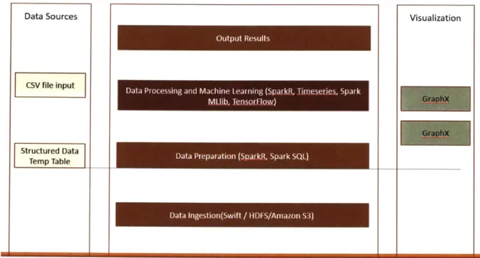
As for the data analytics framework, the data center was built using Apache Spark as the cluster-computing framework. Spark provides an interface for entire clusters with implicit data parallelism and fault tolerance. For distributed storage, Spark can interface with a wide variety of storage options such as OpenStack Swift, Apache Hadoop Distributed File System HDFS), MapR File System (MapR-FS), Apache Cassandra, or Amazon S3. This

etm-allows us to process and analyze data at a large scale leveraging the big data infrastructure set-up.

Data Sources _{Visualization}

Output Results

CSV ile nputData Processing and Machine Learning (5-parkR, Iirnewries, Spark

MUit, Ienwff~low) r

jraphX

Temp Table

Data Ingestion(Swift / HDFS/Amazon S3)

Figure 6 - Big Data Processing with Spark

Spark's in-memory processing is efficient and outperforms Hadoop's speed. While Spark can also perform batch processing, its advantage is at streaming data, interactive queries, real-time data processing, and machine-based learning. Spark's in-memory processing delivers near real-time analytics for data from machine learning, Internet of Things sensors, log monitoring, security analytics, etc. [6] Spark MLlib is fast and efficient distributed machine learning framework on top of the Spark Core and based on the distributed memory-based Spark architecture.

For the experiments discussed in the paper, the two Spark clusters were set up with two master nodes and eight slave nodes. The Apache Zeppelin web-based notebook was set up on a master node for interactive data analytics. Additionally, RStudio Server-side platform was installed for data analytics. The total of 1440 files was uploaded to the server using the Swift protocol and the Spark Jobs were run through the computing clusters with 16 Spark

Figure 6 shows the data processing using Apache Spark and other data analytics and machine learning frameworks.

Cluster Infrastructure

OpenStack/Ubuntu 16.04.4 LTS/Spark 2.2

Job Launch

Assig Tasks Resources

Allocation Worker Node Exctor Resources Allocation Worker Node Executor

Figure 7 - Spark Data Cluster

+- 0 ; ) -I 33*31.2S33.8__ _ _ _- ,-

+*3'-3333 4_A Wa.3.aA 0 OW- A M33Mcwft A OUWIC3N3 A

0.;-

% ;72z.: - ANN

a. -aar* ,n a-,;.eag n-. a 3- 1134 -11

WSfie - 1 te*it/",cnanrnms '.rit- /* = Le~ass i 'I"-,

i 50rn.0 - -Reglle~epf U.0)

,, ,,0,,,e,3 SP35.aa3f3.a.33af..

a. 53.3 333..3.a.A. -eo .. ,. I.,...,.aaaat ts...a.3Wti. '..r -. U '. r 3333

us (.0-It S WM

us nofisic~scse~e

In a EE.3 a.r3.aa.a

-333 a 3uisasta3 3353aar .533r3.31333rasor.Sor 3. 5a3333. 333r'acati~me) o a.3..a3. 3par3.S3'3aaea.33y3.33Ia'))

A =3 -"Gy*- 4r sm, .s.a.033a ma.33/ 3.M3.- 37.3 .

-t ore or :26 MULL * -26 "~ - 16 - -)1-00 - 4)1-

531-' ere :cr"Ve "611u -U' '4243' '43- "31*

.etatastlt:tl 10. * *.@M .13.,'' *t.. .19'r" .9.8-T rol a- .'i -ICV -ICp -- CP-A 33 1 35 *. 33.c'33353' '33ra 91:3.333z" A a.a33.a.3...a,.a.a-....3..,.a.3.33.353.a.3.3a,..., 353W'. Id _{_C 3} Mo.-aa..3. . MerC ei 'udt -4 -v

leat -W -M inc tla (/w/ah/itlttciessedcy

.s3W3e3de3m....-/Nev,.../...5...c 3..3.av

Wft 4ftI 1-1.3a.a.a33f333a5. a.U..W a.3 No.. / W~a/3.. (3,3.33 c

0fta.@N-Oat-/3sa..3*/3ea.438-T130eetd filenams cr [:20) *sta231482-4ten~rgaced~sv""sa.

-.- 1 113M.

as-sed-ltH5swr

Figure 8 -Server-side RStudio

r

DriverSpark

Worker Node

Executor

Worker Node

xecutor

N-~P33 ~ A * 3-.3idwD. A -a.&ba * A &M

4-1

AMrO 2018 .- MwA

Apr4,2 1. 405M4 Apr 11.2, 50

Ias-2.2 Data Flow Pipeline Architecture

Network Data 1fr1 IBM Qfadar provide I

1'

Storing NtokDeft an to Encrypted

has Archived _{syswe ouriary}

OpenStack Swift Dastwo Protocol l

Storage U3 Connector

SparliCiuster

mom Spwr snob o

i ~maew Node

Spark R and PyGMo

SUN"" Nde

Cleaning andn

spr Anlzn

Sk" Nodes

Aggregatsid Det

(hourly dolly and

"IN") _{Tbm series and}

Voeu" stwoftprdctn ru %W O In Gogpy Machine .* I Grfto Multiple ase""" an Predoctions i inborprefto Final Resufs I Fgur..

i

....- .- --F*ue9- P igrm-DtaPpIn

The OPM (Object-Process Methodology) above shows multiple tools, processes, and datasets involved in data analytics and machine learning pipeline and framework. The forms and functions are defined separately to clearly define the tools and products from actions and processing.

2.3 Data Analytics, Machine Learning Tools, and Applications

The research team delved into the predictive power of machine learning with diverse, powerful and efficient algorithms, libraries and frameworks. These machine-Learning techniques will help us establish network traffic baseline, identify network traffic

anomalies, and establish control limits for event accumulation to better alert for the outlier cases. The scalable big data infrastructure built on MIT data center combined with state-of-the-art machine-learning tools allow us to efficiently process large datasets to gain

insightful information.

2.3.lNetwork Traffic Forecasting with Time Series Methods

The Time Series forecasting methods can be used to model data that continues to evolve over time. It performs the forecasting process by analyzing the correlation between the variables such as the volume of data, number of packets and time. The model assumes that certain patterns or combination of patterns will be repeated over the course of time. By identifying and understanding these patterns, the network traffic can be predicted. The model can detect network traffic trend, patterns of communication, seasonal variations and traffic cycles. The different time series models used in this paper are the following:

Non-Seasonal ARIMA -An autoregressive integrated moving average (ARIMA) model is fitted to time series data to predict future values in the series. It is a form

of regression analysis that predicts future movements by examining the differences

between values in the series instead of using the actual data. Lags of the differenced series are referred to as "autoregressive" and lags within forecasted data are referred to as

Non-Seasonal ETS -_{Exponential Smoothing is a forecasting technique using a weighted}

mean of past values with more recent values given higher weights.

Seasonal ARIMA -_{A seasonal ARIMA model is formed by including additional seasonal}

terms in the ARIMA models.

Seasonal ETS -_{A seasonal ETS model is formed by including additional seasonal terms in}

the ETS models.

Double Seasonal Holt-Winters -_{DSHW uses double seasonal exponential methods and it}

is a variation of the Holt-Winters approach with double cycles (daily and weekly). [8]

Multi-Seasonal TBATS -_{TBATS is a more generalized method of DSHW to support}

multiple seasonal forecasting. [8]

Network traffic data gives us the information on the number of packets, data source, destination, and data volume over a time period. Network traffic pattern can be seasonal and the variation in the pattern can provide us with a baseline in network traffic anomaly detection.

Figure 10 - Time Series Network Traffic Data [7]

Thus Smim Pkit of inmi.4 Odmw

-80"

-- =

4 ~* I& li'I? $i"3 i" I

-8"M -ues

2.3.2Network Traffic Forecasting with Long Short-Term

Memory (LSTM) Method

The Long Short-Term Memory network, or LSTM, is a special type of recurrent neural network that can learn and forecast over long sequences. The advantage of LSTMs in addition to learning long sequences is that they can learn to make a one-shot multi-step forecast that can be used for time series forecasting and can be used to improve accuracy in time-series classification. LSTMs can learn the context required to make predictions in time series forecasting problems. By training the network to explicitly choose selective

information to remember, the vanishing gradient does not affect previously kept information.

As shown in Figure 11, LSTMs contain information outside the normal flow of the

recurrent network in a gated cell. The cell makes decisions about what to store, and when to allow reads, writes and deletes via opened and closed gates. [9]

block output

WFMbmr Y 0 - LST+Sode[9

~ith em*4&

+

0

m~~P activaa Fimto

2.3.3Anomaly detection with Bayesian Networks

Bayesian networks are suited for anomaly detection, as they can handle high dimensional data. Some anomalies are visible by plotting individual variables, however, often anomalies are far more subtle and are based on the interaction of many variables. Bayesian statistics provides a framework for combining current observed data with prior assumptions in order to model stochastic systems. Bayesian networks offer the following advantages for anomaly detection: [10]

* Support for both discrete and continuous variables * Support for multi-dimensional models

* Models can contain data which is not time-related and also time series data all within the same model

2.3.4TensorFlow

TensorFlow" is an open source software library for numerical computation and machine learning. It was originally developed by Google's Machine Intelligence research

organization for the purposes of conducting machine learning and deep neural networks research. [11] Our research team worked on the integration of TensorFlow with Apache Spark and Apache Zeppelin web-based notebook for data analytics and processing.

Neural Network Tensorflow Epoch 000,000 Learning rate 0.03 ActIvation - SWgAM Regularization None

6

1 DATA Which datMet do

you want to use?

Ratio of training to teot data: 50% Noisea 0 Batch size: 10 Regularization rate - 0.001 Problem type ClassmfcatIon OUTPUT TOMt tos 0M552 Trrinng oes" 033 K * ** -- 0 -dw. eu & a

13Show test data Q Dacreize output

Figure 12 -Neural Network TensorFlow [12]

2.4 Detecting Network Traffic Anomaly

In the present age of interconnected network, network anomaly detection has become an essential research area, the one that can be aided by big data and machine learning tools. As more and more people and devices get connected over the network, the need for security of information being exchanged increases.

Intrusion Detection System (IDS) is categorized into two major types: Network based IDS (NIDS) and Host-Based IDS (HIDS). The former monitors and analyzes the individual

packets over a network for detecting attacks or malicious activities and the latter examines the activity on an individual computer or host. IDS can also be classified by signature-based detection (recognizing threats such as malware) or anomaly-based detection (detecting deviations from a "normal" traffic, which often relies on machine learning). [13]

Network Behavior Anomaly Detection (NBAD) is the real-time monitoring of a network for unusual activity, trends or events. Tracking of NBAD includes real-time monitoring and alerting. NBAD monitors packets, bytes, flow, frequency, traffic sequence and protocol use.

A baseline of normal network traffic or user behavior must be established over a period of

FEATURES + - 2 HIDDEN LAYERS

Which properties do

-you want to feed In?

4 pmme 2 noma x '511

U

X'W The aL4 AV e~ sin(X,) b sXX

time to be able to identify anomalies when they occur. It is also important to define thresholds to avoid unnecessary alerting of the network traffic.

"Most security monitoring systems utilize a signature-based approach to detect threats. They generally monitor packets on the network and lookfor patterns in the packets which match their database ofsignatures representing pre-identified known security threats. NBAD-based systems are particularly helpful in detecting security

threat vectors in 2 instances where signature-based systems cannot (i) new zero-day attacks (ii) when the threat traffic is encrypted such as the command and control channel for certain Botnets." [14]

The following sections will discuss various approaches to detecting network traffic anomalies that our research team has explored.

2.4.lVolume Based Detection

If we were to analyze the total number of packets and bytes of data between two servers,

we will be able to create a baseline for normal network traffic volume. If the servers are sending and receiving more data than it normally would and outside of the threshold, we can detect data exfiltration (Data Extrusion), botnets (distributed denial of service (DDoS) attack) and lateral movement (progressive network intrusion). Monitoring should be performed on outbound communications data and should trigger an alarm when the suspiciously large amount of data transfer is detected. [15]

S..r..V dat* tran0herrd .aa&8b24:2765:f&64:3238:5758:7c57:53d9 _13236467837 b0ee.1973:425c 746a.9843715.caaaffid _86524401241 b959-av02:3864.87 :ce18 3796d73:574f _4257884762 b198-f1efoa18:cd9d:.471:0016:7b48:7139 _3576000110 ca72:2124:33e:g1191:Odec57o4:abb3:d598 2895778770 ebe:b3a:1720:b4lc:761d:189:1b16:Ib9I _2883936492 c2ce:d661:73bffa3f-98d:lccl:b46e:9520 _2739247339 678a:ebad c81ca739:4240-351l:c57-dac _2494217348 Fhure t3 - r r 10rr tots

Sourc._ P

aaa88b24 27651464 3238.57587c07 03d9

0ee 1973:425c 746a:98d3 715e*ca:af0d

b9.aa02 3864:87d6 ce18:3795:73 574f

b198ieflaaO8 cd9d 9471:0016 7548 7139 b2720cce:092144A17091 890633:66

W.81.521:9808 d8d6:4Id034 c3031.53

8ba79718:715c9bb5:81ae.9e.9567:7723

b56e51973:425c 746a:98d3 7156ftu:ald

Desnm.8nIP 49a4.473de91d6fec:1620.50dd651a0b2 e49-1602:033:65:80c:649d:72893290 .7947e32t45:4814:bdl:112742aa:e325 1d52 c7be:6bef 7018:.22b-165b0487:16ab 2c73 982b:bel:892:0d5655410c588.1 a0dK66876:e04:e411:7b8:7c16:5b4 d&ec 5:7d66:66:b45749:199b:0044 10dd9b21:c795:a3ca:.26:903496743b

Figure 14 - Total Bytes Transferred (Each Source IP)

In the chart below, it shows each Source Machine IP and the summary of the number of distinct Source Ports, Destination Ports, Destination IPs and the Total Number of Bytes transferred. src-Ip 192.168.202.110 192.168.202.83 192.168.202 79 192.168.204.45 192.168.202.68 192.168.20276 192.168.202.81 192.168.202102 dis8~srcpord 62090 28232 9776 16403 75 2844 8503 5258 distdstjol 61949 991 63806 41945 472 47 14 174 distdstjp 2029 3 257 2033 45 142 35 2046 t6taLby0s 277291510 171942757 86487998 55524257 54147421 46956604 2484428 17599261

Figure 15 - Total Bytes Transferred (Port, IP)

2.4.2Time-Based Detection

Through analyzing the network behavior based on time, we can identify anomalies when it deviates from the normal range of activities. Is this server normally busy during the lunch hours of the US East and West coasts? Is there normally less traffic at night or is it higher since there is batch processing at night and weekends? At an individual level, we can determine if a user normally logs-in in the morning and the traffic stops around 5 pm. This allows us to detect patterns such as data exfiltration, insider threats, and lateral movement.

num 13236266793 5635937466 42S6049166 357661348 2420952646 2240148624 2218145131 2211274978

0 5,000,000,000 4,000,000,000 3,000,000,000 2,000,000,000 -1,000,000,000 0

Jul 27, 2017, 10:00:00 PM Jul 27, 2017, 10:01:56 PM Jul 27, 2017, 10:03:52 PM

Figure 16 - Bytes Transferred Based on Time

40,000 - -- -

-5 30,000

25,000

20,000

--Jul 27, 2017, 10:00:00 PM Jul 27, 2017, 10:01:46 PM Jul 27, 2017, 10:03:32 PM

Figure 17 - Number of Connections Based on Time

2.4.3Protocol-Based Detection

Protocol anomalies look at different trends in specific network protocols and send alerts when there are deviations. By analyzing network traffic for port-protocol anomalies, such as outgoing TCP connections to TCP 443 that is not SSL, you can effectively detect

intrusions. [16] "pip -[P kp-ip UPJP kpjp t spip 005006 ". WPOt 0 443 63 80 83 2000 161 23 9997 2054740 804686 620098 608828 464415 319542 312512 173733 r

'30%

7U

Destination_Port * 53 * 80 * 83 M 2"O0 * 181 M 23 * 99F97 M 389 * 06CrM

Figure 19 -Destination Port Usage

2.4.4Geographic and Location Based Detection

Externally facing servers have exposure to be connected to and from all over the globe. It is important to find out a typical pattern of the access. Are your servers local or global?

Where are your customers and vendors who access your servers? Geographic anomaly detection can give you information on advanced persistent threats and phishing attacks.

Figure 20 shows the daily DDoS attack information worldwide based on the geographic

January 17

(I areattac$hs C.y thrted n States

CWAtkBy 9 United*Wte

Size (hndwdt, In Gips) MZ Aj

Sout, Africa

%e(srce + destination)

O mAtdand

dt(Unted~tates).libps DaeaihwnlnG6

ai

Datashrw repesents thetop- 1%of rportedatacfs

Figure 20- Digital Attack Map (Top Daily DDoS Attacks) [17]

2.4.5Network Pattern Based Detection

Network traffic pattern can be defined as a communication trend between two machines or servers, frequency of communication, and pattern of communication. Does Server A

normally talk to Server B? Is this communication followed by Server B connecting to Server

C? If we create a baseline of these trends, we can detect anomalies in these behaviors once

they occur. A usual network behavior of a client machine or a person may be an unusual behavior of another. The tool can detect unauthorized applications, anomalous network activity or applications using unusual ports.

2.5

Experiment Design Selection and Trade Space

As part of the platform, the experiments were conducted using various algorithms and tools. The trade space diagram for architecture and tools selection can be seen in Figure

needed to be performed for both performance and functionality perspectives. The cost is based on ease of use, ease of learning, and overall monetary cost to use the tools.

Architecture-Design Trade Space Diagram

c c 0 c c c 0 c 0 c c 0 0 c C C c C c c C c c 0 0 0 0 0 0 0 9 0 0 0 0 0 c c 0 C C 0 C 0 C 0 C 0 0 * C 0@e ... ccc e 0 0 C. cc C. C. C. C. C. cc 0-@ cC cc C. cc cce c cce @0e cce cce cce c.c cce c c C C 0 c c 0 0 c 0 c c c c c c c c c c 0 0 S S c 0 0 c c c c C 0 c S c 0 0 c c c c cc C C @0 0 maxSChsterA-angemeffn * 2iasters-Workers - 2Masters-4Workers - 1Master-4Workers + Master-2Workers matxSagorihms * EN-ARiMA-ETS ARIMA 0 ErS * * * * * * * * * * * * * * * * 0 SeasonalARIMA * 0 0 0 0 0 0 0 * 0 0 0 0 0 0 0 SeasonalETS ***cC0c c 0 0 ..e TATS cc... .oe Ce DS-Holt-Winters * ** * ** ** 0 0 Anomaly Detecion 0 0 0 0 0 0 LSTM Ccc c _{0 Network} 0 400 500 cost

Figure 21 -Architecture -Tools Trade Space Diagram

Figure 22 shows the available tools for analyzing the data. Highlighted in green are the selections used in this paper. The experiments were done using all of the algorithms in

order to find the ideal solutions to address our predictive models.

Algorithms Ensemble ARIMA ETS Seasonal ARIMA Seasonal ETS TBATS DS-Holt-Winters LSTM Network Parallel Computing Hadoop Spark

Data Storage Amazon S3 Openstack Swift

Compute OpenStack Amazon AWS Databricks

.... ... ... ... ... .... .... .- . . ... - ...- ... ... .... .. .. ... ... .. ... .. ... ... .... ...- .... ... .. .... .. Notebook IDE Rstudlo Zeppelin Sparknotebook Databricks

... ... ... ...

,...-Clusters 2Masters-8Workers 2Masters-4Workers IMaster-4Workers 11Master-2Workers

P... ... .

Py.hn ....

Programming Language: R Python Scala

Figure 22 - Tools Trade Space Selection

5,0- 45-0 S 0 0 C 0 0 C 0 0 0 0 0 0 0 0 c 0 S 0 0 0 0 0 0 0 0 0 0 0 0 0 0 0 0 0 0 0 0 0 0 0 0 0 - 40 r 4.0 35- 0 30- 0 0 0 0 cc .. CCe cce cce cce 00e 0@e @0e 0@o cce 00e 00 0 0 300

3. Experiment: Data Analysis and Engineering

3.1 Data Acquisition and Data Ingestion

As part of data acquisition, we prepared for accessing and processing a large amount of data. The OpenStack Swift was used to upload and store data to the MIT private data

center. The data size is about 5 TB and the files were split into 1440 files (3 - 4 GB each)

before uploading to the Swift container. The data comes in as a CSV file format and the Apache Spark was used as the cluster-computing framework on MIT private data center OpenStack platform.

The OpenStack Object Storage, Swift, is a highly available, distributed, eventually consistent object/blob store. It offers cloud storage software to store and retrieve data using an API. It is optimized for durability, scalability, availability and concurrent processing. [5]

3.2 Data Management

The data is provided in a CSV format retrieved from the IBM QRadar system. For the

network traffic detection to be effective, the solution will need to be processed on real-time data. Apache Spark supports real-time data processing, analytics, and prediction solutions. As data grows over-time, we would need to look into managing data retention, archival and data refresh processes. Real-time data processing is outside the scope of this research project.

3.3 Data Exploration

Table 1 - Data Exploration

Column count: 19 billion records

File Count 1440 Files ( 3-4 GB each)

Total Size About 5 TB

Destination Port, Destination Packets, Destination Bytes,

Destination Flags, Protocol, Category, Source Subnet, Destination Subnet

3.4 Field Descriptions

Table 2 -Field Descriptions

Flow Type Standard Flow -Bidirectional traffic

Type A -Single-to-Many (unidirectional), for example, a single host

that performs a network scan.

Type B -Many-to-Single (unidirectional), for example, a

Distributed DoS (DDoS) attack.

Type C -Single-to-Single (unidirectional), for example, a host to

host port scan.

First Packet Time Specifies the date and time that flow is received.

Last Packet Time Specifies the time that the flow is stored in the QRadar@ database.

Source IP Specifies the source IP address of the flow.

Source Port Specifies the source port of the flow.

Source Packets Specifies the total number of packets that are sent from the source

host.

Source Bytes Specifies the number of bytes sent from the source host.

Source Flags Specifies the Transmission Control Protocol (TCP) flags detected in

the source packet, if applicable.

Destination IP Specifies the destination IP address of the flow.

Destination Port Specifies the destination port of the flow.

Destination Packets Specifies the total number of packets that are sent from the destination host.

Destination Bytes Specifies the number of bytes sent from the destination host.

Destination Flags Specifies the TCP flags detected in the destination packet, if

Protocol _{Specifies the protocol that is associated with the flow.}

Category _{Network traffic category}

Source Subnet _{A logical subdivision of the Source IP network.}

Destination Subnet A logical subdivision of the Destination IP network.

3.5 Data Sampling

Table 3 -Data Sampling

Column _{Sample Data}

Flow Type 1"0" "0" "0"

First Packet Time "1518911823396" "1518911848602" "1518911862841"

Last Packet Time "1518911823480" "1518911859906" "1518911862993"

Source IP "a489063ab5bdccf17f74164e06766a4a" "871be370048c7858849eec983

b0e7e8e"

Source Port "9813" "7654" "11275"

Source Packets "14.0" "2.0" "18.0"

Source Bytes "896.0" "228.0" "1152.0"

Source Flags "26" "31" "31"

Destination IP "4a91dffb43b61aa2919827155acb7a0e" "c6d445630e2d16609eccf2a54

15bc056" Destination Port "443" "53" "443" "443" Destination Packets "10.0" "2.0" "13.0" "11.0" Destination Bytes "640.0" "338.0" "832.0" "704.0" Destination Flags "26" "26" "27" "27" Protocol "TCP" "UDP" "TCP" "TCP"

Category "Web" "Misc" "Web" "Web"

Source Subnet "136.1" "76.96" "136.1"

3.6 Data Encryption

As part of the data analytics process, we need to ensure the security and anonymization of the data. The data is encrypted for certain sensitive information such as IP addresses. We also explored Altastata Client and Admin solutions [18] for file sharing among authorized users. The tool is useful in sharing the data files among users to give exclusive rights to each user to access the data files. It enables high-performance sharing and processing of sensitive big data and JoT data within an AWS or Azure account. Altastata solution

currently supports S3 and Azure Storage and supports parallel processing and streaming of encrypted data integrated with Apache Spark, Kafka, Redis and other programs.

VeraCrypt is another open-source disk encryption software. VeraCrypt features optimized implementations of cryptographic hash functions and ciphers, which boost performance on modern CPUs. It supports parallelized encryption for multi-core systems. The tool was used to encrypt the data files on the hard-drive prior to sending it to the lab for further

4. Experiment: Network Traffic Anomaly Baseline, Prediction,

and Detection

In order to create a baseline of network traffic pattern based on time series, the data was aggregated on an hourly basis. For each timestamp, the aggregated value will show the data transferred among multiple servers. Much of the preparation for analysis involved data cleaning, data aggregation, and data ingestion. The files were split into 1440 files, 18 billion records. The files were uploaded to OpenStack Swift Object Storage. Using Apache SparkR and Server-side RStudio, the files were individually loaded to spark data frames for further processing. Each processing of the file involved data importing, cleaning, splitting, and running model through Spark Clusters following the simplified path below. For the overall

steps, see the Figure 9 -OPM Diagram -Data Pipeline.

Data Pipeline

4.1 Total Volume and Time-Based Anomaly Detection

Time series analysis can be used in many applications for forecasting into the future by using the historical patterns. In our case, the future network traffic will be predicted by examining the historical network traffic trend. By using this baseline, one can detect when network anomalies occur. In this section, the experiment was done based on the total volume of network traffic for each hour for a total of 10 days worth of data.

Figure 24 shows a data plot based on total volume of network traffic for each hour. Here,

the sample data spans 10 days.

Time vs. Total Bytes

C) + ) C) 2018-02-10 00:00:00 2018-02-12 23:27:01 2018-02-15 12:08:06 2018-02-16 19:59:21 2018-02-19 16:52:08 Time

Figure 24 -Time vs. Total Bytes

4.1.lSeasonal ETS Model

-

1-Week Data

The first step of using time series is to see if we can detect seasonality in the data trend. For example, the traffic is likely to be similar on Mondays or during lunchtime on Mondays. The same can be said for the weekend's traffic as well. If we see a variation on the certain uptick of the traffic volume in a certain timeframe, we may be able to identify the anomaly in the trend. Keep in mind that certain increase or decrease of volume does not necessarily mean it is an anomaly or security threat. It may be due to scheduled outages, planned

implementation of new features in the systems or installment of new infrastructure. Discussion of identification of the type of anomaly is outside the scope of this paper. The first model is the seasonal ETS model. Seasonal ETS models work well when the seasonality is present in the dataset. ETS uses exponential smooth for error, trend, and seasonality. The ETS approach detects the additive error and seasonal structures.

4.1.1.1

Data Plot (Time

-

Hours vs. Traffic Volume

-

Bytes

Transferred Count)

10000-Feb 11 Feb 13 Feb 15

TMe

Feb 17 Feb 19

Figure 25 - Time vs. Traffic Volume

As we can see, we have a few peaks in the data volume that are considered anomaly for the purpose of this experiment. We can exclude outliers to clearly define the data trend over time. 7500-E 0 5000 - 250

0-m 0 E 0 5000 -4000 -3000 - 2000-

1000-Feb 11 Feb 13 Feb 15 Feb 17 Feb 19

TOme

Figure 26 -Time vs. Traffic Volume -Excluding Outliers

4.1.1.2

Identifying Multiple Seasonal Levels

The data is volatile showing drastic ups and downs in the diagram with every second timeframe. A moving average concept averages points across several time periods smoothing. 5000 - 4000- 3000- 2000-

1000-Feb 11 Feb 13 Feb 15 Feb 17 Feb 19

tine

Colour

Moving Aterage

- Volume (GB)

Figure 27 - Multiple Seasonal Levels

4.1.1.3

_{Decomposing the Data into the trend and seasonality}

Below, the chart shows the breakdown of trend and seasonality of the data. It is important to decompose a time series into four components: level, trend, seasonality, and remainder (noise). Level describes the average value of the series, the trend is the change in the series from one period to the next, and seasonality describes a short-term cyclical behavior of the series. Noise is a random variation that results from measurement error or other causes.

0 U) (U E' 2 4 8 0 a 10 time

Figure 28 - Decomposing Trend and Seasonality

If there is a trend and/or seasonality, exponential smoothing methods (ETS) works well as

the ETS explicitly models these components. If there is autocorrelation in the data (e.g. the past explains the present), ARIMA methodology may work well. For the purpose of this experiment, ETS, ARIMA, and ENSEMBLE methods were used.

Below, the 5-days worth of data is selected to predict "Friday" forecast. Saturday and Sunday are eliminated due to the unique nature of weekend behavior with much lower traffic. If we were to have multi-week data, we would include weekend-data as well to predict daily and weekly data as it can give more accuracy. ETS forecasting with 24 as a seasonality to reflect the 24-hour seasonality.

4.1.1.4

Seasonal ETS Forecast

E CI 0 C) (0 0) 0) C) 0W 0) CI

Mon Tue Wed Thu Fri Sat

Time

Figure 29 -Seasonal ETS Forecasting

Figure 29 shows the comparison of predicted traffic vs. the observed traffic for the week of

Feb 12. Using the Seasonal ETS Model.

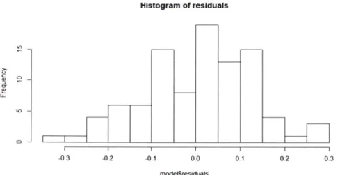
Figure 30 shows the nature of white noise and shows no general trend. This normal

distribution of the residuals shows that the model is correctly specified and no significant autocorrelation is present.

ME -Mean Error is the mean value of errors in a set of predictions. [20]

RSME - Root Mean Squared Error is the square root of the average of squared differences between predicted values and observed values. [20]

MAE - Mean Absolute Error measures the average magnitude of the errors in a set of

predictions, without considering the direction. [20]

MPE - Mean Percentage Error is the computed average of percentage errors of forecasted

values to the observed values. [20] - Original Data

- Seasonal ETS Forecast

/

MAPE - _{Mean Absolute Percentage Error is defined as the volume weighted absolute error}

relative to the total observed values. [20]

SMAPE - _{Symmetric mean absolute percentage error is an accuracy measure based on}

percentage errors. [20]

Table 4 -Seasonal ETS Results - Total Volume -1-Week Data

Seasonal ME RMSE MAE MPE MAPE MASE SMAPE

ETS Results 748.41 1449.86 881.76 12.03 22.81 1.06 13.53

Seasonal ETS Residuals

02- 0.0- -02-i 2 3 4 ₅ 02--- 0.1-0-0 -01 - -0.2--- -03-0 5 10 15 20 25 30 Lag 0.2--- U-0 0~ -0.2--- -0.3-0

II

II I I 5 10 15 20 25 30 Lag

Figure 30 -Seasonal ETS Residuals

0-1

- -

.1

I

.

Histogram of residuals

LL

I I I I I I

-03 -0.2 -0.1 0 0 0.1 0.2 0.3

modeidresiduals

Figure 31 -Seasonal ETS Residual Histogram

Evaluation measures use similar metrics used in the cross-sectional evaluation. MAE, MAPE, and RMSE are the most popular metrics in practice. The results above show that error rates are high partially due to the very limited dataset available.

4.1.1.5

Network Traffic Anomaly Detection

After establishing the baseline and network traffic prediction, it is important to specify the traffic we deem abnormal. The anomaly detection is based on a specific threshold to avoid normal variation in the traffic. It is important to note that the traffic will change over time due to machines being added, the increase or decrease in a number of users, and customer demands based on social, political and economic changes. It is important that these

baselines are re-evaluated and remodeled real-time to reflect regular changes in trend and seasonality.

For the purpose of the research, we will assume that the seasonal ETS model above shows daily volume reasonable for the week chosen. The proposed solution is to define a

threshold using the formula below.

Error Value = Forecasted value - Observed Value

The threshold value can be adjusted to any reasonable ratio based on the volatility of the network trend. Here, we assume .5 as a ratio. It means that if the absolute value of Error Value/Forecast Value is more than .5, meaning the error value is more than 50% of the forecast value, it is considered an anomaly. The diagram below demonstrates the anomalies in the network traffic for the week of 2/10/2018.

0o

0 0V

Mon Tue Wed Thu Fri Sat

Time

Figure 32 -Anomaly Detection (Seasonal ETS)

shows the snapshot of the data that is labeled as anomaly using the method above. -5

Original Data

* Seasonal ETS Forecast

* Anomafles

Table 5 - Labeled Network Traffic Anomaly Data

time index data clean-count count ma forecastedData err abnomaly

49 2018-02-12 00:00-00 8.12874e+11 8.128740e+11 1.237172e+12 1.205689e+12 3.928152e+11 0

50 2018-02-12 01:00:00 8.62984e+11 8.629840e+ 11 1.324512e+12 1.011917e+12 1.489327e+11 0 51 2018-02-12 02:00:00 9.43017e+11 9430170e+11 1.410238e+12 9.754653e+11 3.244833e+10 0 52 2018-02-12 03:00:00 1.04792e+12 1.047920e+12 1.478310e+12 8.711534e+11 -1.767666e+11 0 53 2018-02-12 04:00:00 1.18337e+12 1.183370e+12 1.539175e+12 1.063284e+12 -1.200863e+11 0

54 2018-02-12 05:00:00 1.54593e+12 1.545930e+12 1.592760e+12 1.363325e+12 -1.826051e+11 0 55 2018-02-12 06:00:00 2.14563e+12 2.145630e+12 1.643745e+12 1.717382e+12 -4.282484e+11 0 56 2018-02-12 07:00:00 2.66843e+12 2.668430e+12 1.700482e+12 1.991211e+12 -6.772188e+11 0 57 2018-02-12 08:00:00 2.92654e+12 2.926540e+12 1.772518e+12 2.346129e+12 -5.804107e+11 0 58 2018-02-12 09:00:00 2.29160e+12 2.291600e+12 1.843845e+12 2.519856e+12 2.282561e+11 0 59 2018-02-12 10:00:00 1.93768e+12 1.937680e+12 1.887503e+12 2.600262e+12 6.625818e+11 0 60 2018-02-12 11:00:00 2.59884e+12 2.598840e+12 1.920338e+12 3.156258e+12 5.574178e+11 0 61 2018-02-12 12:00:00 2.71671e+12 2.716710e+12 1.953401e+12 3.375941e+12 6.592313e+11 0 62 2018-02-12 13:00:00 2.89475e+12 2.894750e+12 1.988083e+12 3.762447e+12 8.676967e+11 0 63 2018-02-12 14:00:00 2.51428e+12 2.514280e+12 2.017596e+12 2.819436e+12 3.051555e+11 0

64 2018-02-12 15:00:00 2.05164e+12 2.051640e+12 2.034862e+12 2.454182e+12 4.025423e+11 0

65 2018-02-12 16:00:00 2.12526e+12 2.125260e+12 2.047033e+12 1.925569e+12 -1.996906e+11 0 66 2018-02-12 17:00:00 1.60724e+12 1.607240e+12 2.059683e+12 1.957029e+12 3.497889e+11 0 67 2018-02-12 18:00:00 2.01662e+12 2.016620e+12 2.062298e+12 1.792522e+12 -2.240976e+11 0 68 2018-02-12 19:00:00 1.97233e+12 1.972330e+12 2.042612e+12 4.139293e+12 2.166963e+12 1 69 2018-02-12 20:00:00 2.86143e+12 2.861430e+12 2.002350e+12 1.863198e+12 -9.982319e+11 1 70 2018-02-12 21:00:00 1.95224e+12 1.952240e+12 1.970357e+12 1.802746e+12 -1.A94943e+11 0 71 2018-02-12 22:00:00 1.43614e+12 1.436140e+12 1.962313e+12 1.161616e+12 -2.745240e+11 0 72 2018-02-12 23:00:00 1.35932e+12 1.359320e+12 1.959678e+12 9.971080e+11 -3.622120e+11 0 73 2018-02-13 00:00:00 1.63055e+12 1.630550e+12 1.961224e+12 1.143906e+12 -4.866436e+11 0

4.1.2LSTM Model

-

1-Week Data

In this paper, we have discussed several time-series forecasting techniques such as ETS, ARIMA, Multi-Seasonal TBATS, Double- Seasonal Holt-Winters etc. The Long Short-Term Memory (LSTM) recurrent neural network is used for learning long sequences of

observations that generally works well for the time series forecasting. For this experiment, Keras with TensorFlow backend, Scikit-learn, Pandas, NumPy and Matplotlib libraries were used. The units of the data are in bytes (GB in the results chart), and the timestamp is on an hourly basis. The data is divided into training (4-days) and test (1-day) datasets. The rolling forecast (walk-forward model) is used for the LSTM model. Each time step of the test dataset is calculated one at a time. A model is used to make a forecast for the time step, and then the actual expected value from the test set is fed into the model for the forecast on the next time step. [21]

- Observed Data - Total Bytes- - _{Predicted - LSTM Forecast}

f00yf,

20 40 1 I I I ii 1 I 80 100

Figure 33 - LSTM Forecasting - 1-Week Data

1.a0 0.8 - 0.6-0.4 O.2 - 0.0-120

7-5 4 3 2 1 0

-- Observed Data - Total Bytes- - Predicted - LSTM Forecast

1%

05 10 15 0

Figure 34 -LSTM Forecasting -1-Week Data

Table 6 - LSTM Results -Total Volume -1-Week Data

LSTM ME RMSE MAE MPE MAPE MASE SMAPE

Results 1531.54 1005.19 31.062

In this example, LSTM forecast seems to perform worse than the Seasonal ETS model for the 1-week data. LSTM forecast generally performs better in larger datasets as it needs substantial historical data to make accurate predictions.