Dynamic Reconfiguration of Visuomotor-Related Functional Connectivity Networks

HAL Id: hal-02088316

https://hal-amu.archives-ouvertes.fr/hal-02088316

Submitted on 2 Apr 2019

HAL is a multi-disciplinary open access

archive for the deposit and dissemination of

sci-entific research documents, whether they are

pub-lished or not. The documents may come from

teaching and research institutions in France or

abroad, or from public or private research centers.

L’archive ouverte pluridisciplinaire HAL, est

destinée au dépôt et à la diffusion de documents

scientifiques de niveau recherche, publiés ou non,

émanant des établissements d’enseignement et de

recherche français ou étrangers, des laboratoires

publics ou privés.

Functional Connectivity Networks

Andrea Brovelli, Jean-Michel Badier, Francesca Bonini, Fabrice Bartolomei,

Xolivier Coulon, Guillaume Auzias

To cite this version:

Andrea Brovelli, Jean-Michel Badier, Francesca Bonini, Fabrice Bartolomei, Xolivier Coulon, et al..

Dynamic Reconfiguration of Visuomotor-Related Functional Connectivity Networks. Journal of

Neu-roscience, Society for NeuNeu-roscience, 2017, �10.1523/JNEUROSCI.1672-16.2016�. �hal-02088316�

Behavioral/Cognitive

Dynamic Reconfiguration of Visuomotor-Related Functional

Connectivity Networks

X

Andrea Brovelli,

_X

_{Jean-Michel Badier,}

_{Francesca Bonini,}

_{Fabrice Bartolomei,}

_X

_{Olivier Coulon,}

_*

and

X

Guillaume Auzias

_*

1_{Institut de Neurosciences de la Timone, Unite´ Mixte de Recherche 7289, Aix Marseille Universite´, Centre National de la Recherche Scientifique, 13385} Marseille, France;2_{Aix Marseille Universite´, Institut de Neurosciences des Systèmes Unite´ Mixte de Recherche Scientifique 1106, 13005 Marseille, France;} 3_{Inserm, Unite´ Mixte de Recherche Scientifique 1106, 13005 Marseille, France; and}4_{Aix-Marseille Universite´, Centre National de la Recherche Scientifique,} Laboratoire des Sciences de l’Information et des Systèmes Unite´ Mixte de Recherche 7296 Marseille, France

Cognitive functions arise from the coordination of large-scale brain networks. However, the principles governing interareal functional

connectivity dynamics (FCD) remain elusive. Here, we tested the hypothesis that human executive functions arise from the dynamic

interplay of multiple networks. To do so, we investigated FCD mediating a key executing function, known as arbitrary visuomotor

mapping, using brain connectivity analyses of high-gamma activity recorded using MEG and intracranial EEG. Visuomotor mapping was

found to arise from the dynamic interplay of three partly overlapping cortico-cortical and cortico-subcortical functional connectivity

(FC) networks. First, visual and parietal regions coordinated with sensorimotor and premotor areas. Second, the dorsal frontoparietal

circuit together with the sensorimotor and associative frontostriatal networks took the lead. Finally, cortico-cortical interhemispheric

coordination among bilateral sensorimotor regions coupled with the left frontoparietal network and visual areas. We suggest that these

networks reflect the processing of visual information, the emergence of visuomotor plans, and the processing of somatosensory

reaffer-ence or action’s outcomes, respectively. We thus demonstrated that visuomotor integration resides in the dynamic reconfiguration of

multiple cortico-cortical and cortico-subcortical FC networks. More generally, we showed that visuomotor-related FC is nonstationary

and displays switching dynamics and areal flexibility over timescales relevant for task performance. In addition, visuomotor-related FC

is characterized by sparse connectivity with density

⬍10%. To conclude, our results elucidate the relation between dynamic network

reconfiguration and executive functions over short timescales and provide a candidate entry point toward a better understanding of

cognitive architectures.

Key words: dynamic reconfiguration; executive functions; functional connectivity dynamics; high-gamma activity; MEG; SEEG

Introduction

The dynamic coordination of neural activity over large-scale

net-works is thought to support cognitive functions (Varela et al.,

2001;

Bressler and Menon, 2010;

von der Malsburg et al., 2010).

Growing evidence from fMRI has shown that spontaneous and

task-related activity is composed of multiple and spatially

over-lapping subnetworks that dynamically evolve over tens of

sec-onds to minutes (Hutchison et al., 2013;

Yeo et al., 2014;

Allen et

Received May 17, 2016; revised Nov. 3, 2016; accepted Nov. 12, 2016.

Author contributions: A.B. designed research; A.B., J.-M.B., and F. Bonini performed research; A.B., F. Bartolomei, O.C., and G.A. contributed unpublished reagents/analytic tools; A.B. analyzed data; A.B., O.C., and G.A. wrote the paper.

This work was partly supported by Projets Exploratoires Pluridisciplinaires (PEPS) from the Centre National de la Recherche Scientifique/Inserm/Inria “Bio-math-Info” entitled “Computational and neurophysiological bases of goal-directed and habit learning.” and was performed on an MEG platform member of France Life Imaging network

Significance Statement

Executive functions are supported by the dynamic coordination of neural activity over large-scale networks. The properties of

large-scale brain coordination processes, however, remain unclear. Using tools combining MEG and intracranial EEG with brain

connectivity analyses, we provide evidence that visuomotor behaviors, a hallmark of executive functions, are mediated by the

interplay of multiple and spatially overlapping subnetworks. These subnetworks span visuomotor-related areas, the

cortico-cortical and cortico-subcortico-cortical interactions of which evolve rapidly and reconfigure over timescales relevant for behavior.

Visuomotor-related functional connectivity dynamics are characterized by sparse connections, nonstationarity, switching

dy-namics, and areal flexibility. We suggest that these properties represent key aspects of large-scale functional networks and

cognitive architectures.

al., 2014;

Calhoun et al., 2014;

Cole et al.,

2014;

Zalesky et al., 2014;

Hansen et al.,

2015). Indeed, dynamic network

recon-figuration has been suggested to

repre-sent a fundamental neurophysiological

process supporting executive function

(Bassett et al., 2011;

Braun et al., 2015).

A hallmark of executive function is the

ability to rapidly associate arbitrary

ac-tions to visual inputs and internal goals.

This ability, known as arbitrary

visuomo-tor mapping, recruits a large-scale

net-work comprising the sensorimotor and

frontoparietal circuits, in addition to

me-dial prefrontal areas and basal ganglia

(Wise et al., 1996;

Murray et al., 2000;

Passingham et al., 2000;

Wise and Murray,

2000;

Hadj-Bouziane et al., 2003;

Petrides,

2005). In the current study, the goal was to

investigate whether visuomotor mapping

results from the dynamic interplay of

multiple subnetworks. More precisely, we

tested the hypothesis that multiple

sub-networks reconfigure in a dynamic

fash-ion over timescales relevant for executive

behaviors.

To do so, we exploited the

high-gamma activity (HGA; ranging from

⬃60

to 150 Hz), which reflects

population-level local neural activity (Ray et al., 2008;

Ray and Maunsell, 2011). In humans,

power modulations in the HGA range are

commonly recorded using MEG and

in-tracranial EEG to map task-related brain

regions (Brovelli et al., 2005;

Crone et al.,

2006;

Vidal et al., 2006;

Ball et al., 2008;

Jerbi et al., 2009;

Darvas et al., 2010;

Lachaux et al., 2012;

Cheyne and Ferrari,

2013;

Ko et al., 2013). In addition,

high-gamma-power modulations can be used

to characterize functional connectivity

(FC) among brain regions supporting

executive functions (Brovelli et al.,

2015).

Here, we predicted visuomotor mapping to reflect an initial

activation of visual circuits mediating the processing of sensory

input, followed by frontoparietal and motor networks for

visuo-motor integration and visuo-motor planning. We tested these

hypoth-eses in a group of healthy participants during MEG recordings by

combining FC analysis of atlas-based HGA with methods from

network science and graph theory. In particular, we investigated

the presence of multiple visuomotor-related spatiotemporal

pat-terns through the analysis of FC dynamics (FCD). Intracranial

assessment of HGA activations from MEG was also performed in

three epileptic patients performing the same task during

stereo-EEG (Sstereo-EEG) recordings.

Materials and Methods

Experimental procedure and data acquisition

Experimental conditions and behavioral tasks. Eleven healthy participants

and three epileptic patients accepted to take part in our study. Healthy participants were right handed and the average age was⬃23 years (SD ⫽ 3.8 years); 4 were females and 7 males. All gave written informed consent according to established institutional guidelines and local ethics commit-tee, and received monetary compensation (€50). Three patients (one right-handed female age 29, two right-handed males age 29 and 43) undergoing presurgical evaluation of drug-resistant epilepsy (Epilepsy Unit, La Timone Hospital, Marseille, France) participated in this study. They all gave their informed consent before their participation. The SEEG study was approved by the institutional review board of the French Institute of Health. Healthy participants and patients performed the same behavioral task. Participants were asked to perform an associative visuomotor mapping task in which the relation between visual stimulus and motor response is arbitrary and deterministic (Wise and Murray, 2000;Brovelli et al., 2015). As shown inFigure 1A, the task required

(Grant ANR-11-INBS-0006). We thank Faical Isbaine and Sophie Chen for help with the MEG experiments and Patrick Marquis and Catherine Liegeois-Chauvel for help with the SEEG experiments.

The authors declare no competing financial interests. *O.C. and G.A. contributed equally to this work.

Correspondence should be addressed to Andrea Brovelli, Institut de Neurosciences de la Timone (INT), UMR 7289 CNRS, Aix Marseille University, Campus de Sante´ Timone, 27 Bd. Jean Moulin, 13385 Marseille, France. E-mail: andrea.brovelli@univ-amu.fr.

DOI:10.1523/JNEUROSCI.1672-16.2016

Copyright © 2017 the authors 0270-6474/17/370840-15$15.00/0

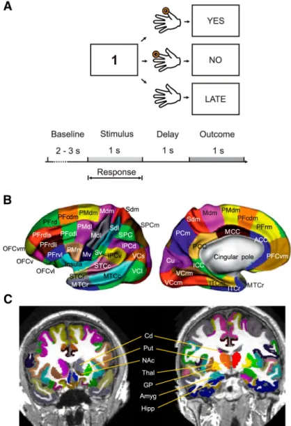
Figure 1. A, Arbitrary visuomotor mapping task. B, MarsAtlas: cortical parcellation displaying the anatomical gradients both in

the rostrocaudal and dorsoventral directions; for a detailed description, seeAuzias et al. (2016). C, MarsAtlas: single-subject exemplar volumetric representation displaying subcortical regions included in the atlas: nucleus accumbens, amygdala, hip-pocampus, globus pallidus, putamen, caudate nucleus, and thalamus.

participants to perform a finger movement associated to a digit number: digit “1” instructed the execution of the thumb, “2” for the index finger, “3” for the middle finger, and so on. Maximal reaction time was 1 s. After a fixed delay of 1 s after the disappearance of the digit number, an out-come image was presented for 1 s and informed the subject whether the response was correct, incorrect, or too late (if the reaction time exceeded 1 s). Incorrect and late trials were excluded from the analysis because they were either absent or very rare (i.e., maximum two late trials per session). The next trial started after a variable delay ranging from 2 to 3 s (rdomly drawn from a uniform distribution) with the presentation of an-other visual stimulus. Each participant performed two sessions of 60 trials each (total of 120 trials). Each session included three digits ran-domly presented in blocks of three trials. The average reaction time was 0.504⫾ 0.004 s (mean ⫾ SEM).

Anatomical, functional, and behavioral data acquisition in healthy participants. Anatomical MRI images were acquired for healthy

partici-pant using a 3 T whole-body imager equipped with a circular polarized head coil. High-resolution structural T1-weighted anatomical image (inversion-recovery sequence, 1⫻ 0.75 ⫻ 1.22 mm) parallel to the ante-rior commissure–posteante-rior commissure plane, covering the whole brain, were acquired. MEG recordings were performed using a 248 magnetom-eters system (4D Neuroimaging Magnes 3600). Visual stimuli were pro-jected using a video projection and motor responses were acquired using a LUMItouch optical response keypad with five keys. Presentation soft-ware was used for stimulus delivery and experimental control during MEG acquisition. Reaction times were computed as the time difference between stimulus onset and motor response. Sampling rate was 2034.5 Hz. Location of the participant’s head with respect to the MEG sensors was recorded both at the beginning and end of each session to exclude sessions and/or participants with large head movements. For each session and participant, the displacement between the beginning and end of a session was computed. A supine position was chosen to minimize head movements. This cutoff was decided by considering the spatial distance between sources (5 mm), as described in the following sections. None of the participants moved⬎3 mm during all sessions. Therefore, all partic-ipants were considered for further analysis.

Anatomical, functional, and behavioral data acquisition in epileptic pa-tients. The surgical treatment of drug-resistant epilepsy may require

di-rect intracerebral recording of cortical activity IEEG in multiple brain areas to localize the epileptic tissue to be removed. Before SEEG, all patients had high-resolution MRI performed with a 3 T Siemens Magne-tom scanner, including a 3D T1-weighted acquisition. Intracerebral multiple contacts electrodes (10 –15 contacts, length: 2 mm, diameter: 0.8 mm, 1.5 mm apart) were implanted using a stereotactic method. A postoperative computerized tomography (CT) scan without contrast was used to verify the absence of bleeding and the location of each re-cording lead. During this presurgical evaluation period, patients were asked to participate in our behavioral protocol at the Timone Hospital. They were seated in a Faraday cage and stimuli were presented on a display monitor at 70 cm to patient’s eyes with an angular size of 1.26°. Presentation software was used for stimulus delivery and experimental control during SEEG acquisition. Motor responses were acquired using a five-button response pad. SEEG signals were acquired on referential montage with a sampling frequency of 1000 Hz and an acquisition band-pass filter between 0.1 and 200 Hz.

Brain parcellation

To map brain activations and FC patterns to specific anatomical brain networks, single-subject brain parcellation can be created from macro-anatomical information, such as primary and secondary sulci using ei-ther volume-based (Lancaster et al., 2000;Tzourio-Mazoyer et al., 2002) or surface-based (Van Essen and Drury, 1997;Fischl et al., 2002;Desikan et al., 2006) algorithms. Recent developments now allow single-subject cortical parcellation complying with a model of anatomofunctional gra-dients in the rostrocaudal and dorsoventral directions (Auzias et al., 2013) optimized for functional mapping using HGA (Auzias et al., 2016). Such an approach allows group-level analyses and comparison between individual patients and healthy participants in control group. We created a whole-brain parcellation including cortical (Fig. 1B) and subcortical

(Fig. 1C) regions based on macro-anatomical information. The

identifi-cation of the cortical regions requires several processing steps. After denoising using a nonlocal means approach (Coupe´ et al., 2008), T1-weighted MR-images were segmented using the FreeSurfer “recon-all” pipeline共http://freesurfer.net兲. Gray and white matter segmentations of

each hemisphere were imported into the BrainVisa software and pro-cessed using the Morphologist pipeline procedure共http://brainvisa.info兲.

White matter and pial surfaces were reconstructed and triangulated and all sulci were detected and labeled automatically (Mangin et al., 2004; Perrot et al., 2011). A parameterization of each hemisphere white matter mesh was performed using the Cortical Surface Toolbox 共http://brainvisa.info/web/cortical_surface.html兲. This resulted in a 2D

orthogonal system defined on the white matter mesh constrained by a set of primary and secondary sulci (Auzias et al., 2013). This parameteriza-tion naturally leads to a complete parcellaparameteriza-tion of the cortical surface, the

MarsAtlas model (Auzias et al., 2016).

MarsAtlas complies with the dorsoventral and rostrocaudal trends of

cortical organization (Pandya and Yeterian, 1985;Re´gis et al., 2005) and provides a good level of both functional segregation and intersubject matching for functional analysis using single-trial MEG HGA (Auzias et al., 2016). The resulting cortical surface parcellation was then propagated to the volume-based gray matter segmentation using a front propagation from the surface through the volumetric cortex segmentation (Cachia et al., 2003), thus producing a volume-based parcellation of the entire cor-tex. The parcels corresponding to the subcortical structures were ex-tracted using Freesurfer (Fischl et al., 2002). The subcortical structures included in the brain parcellation were the caudate nucleus, putamen, nucleus accumbens, globus pallidus, thalamus, amygdala, and hip-pocampus. The whole-brain parcellation therefore comprised 96 areas (41 cortical and 7 subcortical areas per hemisphere;Fig. 1). All of these processing steps can be performed using the BrainVisa neuroimaging platform共http://brainvisa.info/web/index.html兲. MarsAtlas is included

in the cortical surface toolbox.

Single-trial HGA in MarsAtlas

Preprocessing and spectral analysis of MEG and SEEG signals. The

prepro-cessing and spectral analyses steps for MEG and SEEG signals were identical. Concerning SEEG signals, an electrode’s contacts in the epilep-togenic zone were excluded from the analysis. SEEG contacts outside of the epileptogenic zone were chosen for analysis. In addition, epochs with signs of epileptic activity were removed. MEG and SEEG signals were first down-sampled to 1 kHz, low-pass filtered to 250 Hz, and then segmented into epochs aligned on finger movement (i.e., button press). Epoch seg-mentation was also performed on stimulus onset and the data from⫺0.5 and⫺0.1 s before stimulus presentation were taken as baseline activity for the calculation of the single-trial HGA. Artifact rejection was performed semiautomatically and by visual inspection. For each movement-aligned epoch and channel, the signal variance and z-value were computed over time and taken as relevant metrics for the identifi-cation of artifact epochs. All trials with a variance⬎1.5*10–24 across channels were excluded from further search of artifacts. Metrics such as the z-score, absolute z-score, and range between the minimum and max-imum values were also inspected to detect artifacts. Channels and trials displaying outliers were removed. Two MEG sensors were excluded from the analysis for all subjects.

Spectral density estimation was performed using multitaper method based on discrete prolate spheroidal (slepian) sequences (Percival and Walden, 1993;Mitra and Pesaran, 1999). To extract HGA from 60 to 120, MEG time series were multiplied by k orthogonal tapers (k⫽ 8) (0.15 s in duration and 60 Hz of frequency resolution, each stepped every 0.005 s), centered at 90 Hz and Fourier-transformed. Complex-valued estimates of spectral measures,Xsensorn 共t, k兲, including cross-spectral density

matri-ces, were computed at the sensor level for each trial n, time t, and taper k.

MEG source analysis and HGA. Source analysis requires a physical

forward model or lead field, which describes the electromagnetic relation between sources and MEG sensors. The lead field combines the geomet-rical relation of sources (dipoles) and sensors with a model of the con-ductive medium (i.e., the head model). For each participant, we generated a head model using a single-shell model constructed from the

segmentation of the cortical tissue obtained from individual MRI scans (Nolte, 2003). Lead fields were not normalized. Sources were placed in the single-subject volumetric parcellation regions. For each region, the number of sources nSP was computed as the ratio of the volume and the volume of a sphere of radius equal to 3 mm. The k-means algorithm (Tou and Gonzalez, 1974) was then used to partition the 3D coordinates of the voxels within a given volumetric region into nS clusters. The sources were placed at the center of each partition for each brain region. The head model, source locations and the information about MEG sensor position for both models were combined to derive single-participant lead fields. The orientation of cortical sources was set perpendicular to the cortical surface, whereas the orientation for subcortical sources was left unconstrained.

Adaptive linear spatial filtering (Van Veen et al., 1997) was used to estimate the power at the source level. The dynamical imaging of coher-ent sources (DICS) method was used, a beam-forming algorithm for the tomographic mapping in the frequency domain (Gross et al., 2001), which is well suited for the study of neural oscillatory responses based on single-trial source estimates of band-limited MEG signals (for a series of reviews, seeHansen et al., 2015). At each source location, DICS uses a spatial filter that passes activity from this location with unit gain while maximally suppressing any other activity. The spatial filters were com-puted on all trials for each time point and session and then applied to single-trial MEG data. DICS allows the estimate of complex-value spec-tral measures at the source level,Xsourcen 共t, k兲 ⫽ A共t兲Xsensorn 共t, k兲, where

A(t) s the spatial filter that transforms the data from the sensor to source

level andXsensorn 共t, k兲is the complex-valued estimates of spectral

mea-sures, including cross-spectral density matrices, computed at the sensor level for each trial n, time t, and taper k (for a detailed description of a similar approach, seeHipp et al., 2011). The single-trial high-gamma power at each source location was estimated by multiplying the complex spectral estimates with their complex conjugate, and averaged over tapers

k,Psourcen 共t兲 ⫽ 具Xsourcen 共t, k兲Xsourcen 共t, k兲*k典, where angle brackets refer to the

average across tapers and * to the complex conjugate. Single-trial power estimates aligned on movement and stimulus onset were log transformed to make the data approximate Gaussian and low-pass filtered at 50 Hz to reduce noise. Single-trial mean power and SD in a time window from ⫺0.5 and ⫺0.1 s before stimulus onset was computed for each source and trial and used to z-transform single-trial movement-locked power time courses. Similarly, single-trial stimulus-locked power time courses were log transformed and z-scored with respect to baseline period to produce HGAs for the prestimulus period from⫺1.6 to ⫺0.1 s with respect to stimulation for subsequent FC analysis. Finally, single-trial HGA for each brain region of MarsAtlas was computed as the mean z-transformed power values averaged across all sources within the same region.

SEEG localization and HGA. Electrodes were localized using the CTMR

toolbox (Hermes et al., 2010). Briefly, postimplant CT scans were coreg-istered and resliced to the MRI coordinate scans of each subject using SPM12. A manual procedure was then performed to mark the electrodes in the co-registered CT space using the CTMR toolbox. The coordinates of each electrode were transformed to MRI space (1 mm resolution). Because bipolar derivations were used, the coordinates of the midpoint between pairs of adjacent electrodes were computed. A cube of 5 mm in size was placed at these positions (i.e., at the position of the bipolar derivation) and each voxel of the cube (1 mm resolution) was labeled according to MarsAtlas. The location of each bipolar derivation was then labeled according to the label associated to the largest number of voxels within the cube. Bipolar derivations labeled in the white matter were excluded from further analyses.

Similarly to MEG HGA estimation, single-trial power estimates in the high-gamma range (60 –120 Hz) aligned on movement and stimulus onset were log transformed and low-pass filtered at 50 Hz to reduce noise. Single-trial estimates of high-gamma power were z-transformed with respect to baseline period from⫺0.5 and ⫺0.1 s before stimulus onset. Finally, single-trial HGA for each labeled brain region of MarsAtlas was defined as the mean z-transformed power values averaged across all electrodes within the same region.

Single-trial FCD measures

Power modulations in the high-gamma range reflect the activity of local neural populations (Ray et al., 2008;Ray and Maunsell, 2011). Here, we assume that tracking statistical dependencies between HGA from differ-ent brain regions provides information about how local processing units coordinate at the large-scale level during cognitive tasks. The goal is not infer the mechanisms mediating interareal communication. This would require complementary approaches based on the study of role of neural oscillations and synchrony for interregional communication (Fries, 2015;Buzsa´ki and Schomburg, 2015). Rather, the aim was to map task-related FCD onto anatomical circuits. Given the sparseness of brain regions sampled with SEEG, FCD was performed exclusively for whole-brain MEG data.

Linear correlation analysis was used to study the FC between brain regions. To quantify the evolution of FC over time (i.e., FCD), the Pear-son’s correlation coefficient between pairs of HGA signals over sliding windows of 500 ms stepped every 10 ms was computed. The same pro-cedure was performed across all pairs of brain regions and for each trial. This resulted in a 4D FCD matrix (i.e., regions⫻ regions ⫻ time points ⫻ trials) representing the evolution of linear correction across all pairs of brain areas from⫺0.7 to 0.7 s around movement onset. The single-trial FCD matrix was also computed during the prestimulus period, from ⫺0.8 to ⫺0.1 s before stimulus onset for baseline. Statistical analyses searched for significant modulations in movement-related FCD with respect to those in the prestimulus interval.

Statistical analysis

Linear mixed effect (LME) model. Statistical inference of single-trial

HGAs was performed using an LME model approach at the group level. A LME model was used because they are particularly suited for the analysis of data collected from multiple subjects (or sessions) for which it is important to take into account interindividual variability. These models formalize the relation between a response variable and independent variables using both fixed and random effects. Fixed effects model the response variable in terms of explanatory variables as nonrandom quantities. For example, experimental conditions re-lated to population mean may be considered as fixed effects. Random effects are associated with individual experimental units drawn at random from a population, which may correspond to different par-ticipants in the study (or experimental sessions). In other words, whereas fixed effects are constant, random effects are drawn from a prior known distribution. A LME model is generally expressed in matrix formulation as follows:

y⫽ X␤ ⫹ Zb ⫹ e (1)

where y is the n-by-1 response vector and n is the number of observa-tions, x is an n-by-p fixed-effects design matrix, and␤ is the fixed-effect vector of p-by-1, where p is the number of fixed effects, z is an n-by-q random-effects design matrix, and b is a q-by-1 random-effects vector, where q is the number of random effects and e is the n-by-1 observation error. The random-effects vector, b, and the error vector, e, were assumed to be drawn from independent normal distributions. Parameter esti-mation was performed using maximum likelihood method, using the

fitlme.m function in the Statistical Toolbox of MATLAB (The

Math-Works). To test for significant modulations in single-trial HGA and FCD measures around movement onset with respect to the baseline period, a random-intercept and random-slope LME model was used as described by the following:

y共t兲 ⫽␤0共t兲 ⫹␤1共t兲 xj⫹ b0j共t兲 ⫹ b1j共t兲 zj⫹ ␧j共t兲 (2)

wherey共t兲 ⫽ 关ybl共1兲, ybl共2兲, . . ., ybl共np兲, ymv共1, t兲,ymv共2, t兲, . . ., ymv共np, t兲兴.

For MEG data analysis,ybl共j兲was a vector containing the baseline

neural activity (i.e., the HGA from single brain regions or FCD values for single pairs of regions) for all trials and sessions (i.e., data from both sessions were concatenated, because they were acquired in uninterrupted succession) for subject j⫽ 1,2 . . . np, where np is the number of partic-ipants at time instant t. Note that t does not refer to trials, but rather the

time within each trial.ymv共j, t兲was a vector including brain activity

across all trials for subject j at time t with respect to movement onset. For SEEG data analysis, statistical inference was performed at the single-participant level due to the limited number of patients and limited sampling of MarsAtlas regions. However, given that the SEEG experi-ments were composed of two sessions acquired at different times (⬃1 h interval), we modeled sessions as random effects.ybl共j兲was then a vector

containing the baseline neural activity (i.e., the HGA from single brain regions) for all trials for sessions j⫽ 1,2 at time instant t. As before, t did not refer to trials, but time within each trial.ymv共j, t兲was a vector

includ-ing brain activity across all trials for session j at time t with respect to movement onset.

The following statistical analysis was similar for both MEG and SEEG data. The design matrices contain two columns. The first column is a vector of ones to model the intercept, and thus it was eliminated from Equation 2. The second column contains negative ones for baseline trials and ones for event-related trials, therefore modeling the change with respect to baseline, or slope, and it is referred as xjand zjin Equation 2.

Therefore, the first and third terms in the right side of Equation 2 model the intercepts, which correspond to the mean values between baseline and movement-related activity. The second and fourth terms model the slopes, which are the differences between baseline and movement-related activity. The␤1(t) values are fixed across subjects, whereas the b1j(t)

values model the random variations across subjects (for MEG) or ses-sions (for SEEG). In other words, the parameter␤1(t) models the change

in neural activity (e.g., HGA or FCD for MEG data) with respect to baseline at each time point t at the group level; the parameter b1j(t)

models the change in neural activity with respect to baseline for each participant (or sessions) j and therefore explains the across-subjects (or across-session) variability for MEG and SEEG data, respectively. The across-subject and across-session variability was considered of no inter-est for the scope of the current analyses. We thus analyzed fixed effects. Given the structure of the fixed-effect design matrix, significant differ-ences in movement-related neural activity with respect to baseline can thus be inferred by testing whether ␤1 coefficients are significantly

greater than zero. More formally, the significance of movement-related modulations was inferred using a t test by testing the null hypothesis H0:

␤1ⱕ 0.

Statistical inference was performed for each time point t and each brain area for the analysis of HGAs. To account for the multiple-comparisons problem, the false discovery rate (FDR) was controlled (Benjamini and Yosef, 1995). For mean HGA statistical analyses, the number of time points and brain regions were corrected for; for FCD analyses, the number of time points and for the number of pairs of brain regions were corrected for. To further assess the validity of our results, the minimum number of consecutive significant time points required to reject a null hypothesis of absence of a cluster given a chance probability

p0⫽ 0.5 (two possible outcomes, significant or nonsignificant) were

quantified and only those clusters with a duration that exceeded a given significance level were kept. Details of the calculation are given in the appendix ofSmith et al. (2004).

The statistical analyses of MEG HGA modulations resulted in a group-level FCD matrix containing time-evolving t- and p-values for each brain region in MarsAtlas (whole-brain analysis). For brain regions covered by the SEEG implants, the analysis of HGA modulations produced intracra-nial validation at the single-participant level. The analysis of FCD from MEG HGA produced t- and p-value time courses for all pairs of brain regions.

Graph theoretical analysis

Strength of functional link (SFL). To gain insight into the topology of the

task-related functional network arising from group-level MEG analyses, graph theoretical analyses of the FCD matrix containing the p-values associated with the LME analysis were performed. The weight or strength of the evidence of a functional link was defined as the minimum Bayes factor (BF) associated with such p-values (Goodman, 1999b). The ratio-nale behind the transformation of p-values to minimum BFs is an at-tempt to move toward statistical measures that can be better interpreted (Goodman, 1999a). The BF is a convenient measure of the strength of

statistical evidence and it can be computed from p-values asBFup ⬍ ⫺1/

共e p ln共p兲兲if p-values satisfy the relation p⬍ 1/e, in which e ⬇ 2.72. This estimate provides an upper bound (BF_up) on the BF, and it can be thought as providing an “optimistic” limit of the BF for a given p-value (Goodman, 2001; Stephens and Balding, 2009). BFs were log trans-formed to give a measure that quantifies the strength in the evidence of the presence of a functional link between two brain regions,SFL ⫽ log10 BFup. The SFL matrix has the same dimensions of group-level FCD matrix

(i.e., regions⫻ regions ⫻ time points). A value between 1 and 2 can be interpreted as providing strong to very strong evidence of a functional link (i.e., increase in correlation with respect to baseline), whereas a value ⬎2 is interpreted as decisive.

Analysis of time-averaged and time-dependent SFL. A caveat of FC

analysis is the dependence of functional links on the threshold chosen for statistical significance. Therefore, to explore how graph theoreti-cal measures vary according to significance levels, the SFL matrix was multiplied with different binary masks obtained from the FDR cor-rection of the FCD matrix over a wide range from highly significant values ( p_{FDR-corrected}⫽ q ⬍ 0.001) to nonsignificant (q ⬍ 0.99999). Note that a FDR-adjusted p-value is denoted as a q-value. This pro-duced several thresholded SFL matrices, each one associated with a given level of significance.

As a first analysis, the mean SFL matrices were computed over time, thus giving an adjacency matrix (regions⫻ regions) representing the mean strength between brain regions at different significance levels. The density D (the ratio between the number of functional links and the number of possible connections) was computed as a function of the

q-value. In addition, to identify the most important brain regions in

average SFL graph, the strength of each region (sum of functional links of a region) and two indicators of centrality, such as the eigenvector cen-trality EC, defined as the absolute value of the eigenvector associated with the largest eigenvalue of the adjacency matrix W and it measures the importance of a region, and the between-ness centrality (BC), which is equal to the fraction of all shortest paths that pass through a given region, so it measures the number of times a region that acts as a “bridge” were computed. These measures were, however, computed only at q⬍ 0.05. Finally, to evaluate the evolution of density of the thresholded FCD, it was computed for each time slice rather over the averaged FCD. Graph theoretical measures were computed using the Brain Connectivity Tool-box (Rubinov and Sporns, 2010).

Detection of functional subnetworks. A critical step in the analysis of

brain networks is the detection of communities, which may correspond to functional subnetworks. Subnetworks, however, may overlap spa-tially, such that a given brain region may belong to more than one group. Link communities, defined as groups of links rather than nodes, provide an appropriate framework for capturing the relationships between over-lapping communities while revealing hierarchical organization (Ahn et al., 2010). To detect time-varying link communities, an approach based on the analysis of the correlation of edge weights over time, rather than nodes, was used, similarly to previous works analyzing “cross-links” or “hyper-edges” (Bassett et al., 2014;Davison et al., 2015).

First, the Pearson linear correlation between significant (at q⬍ 0.05) pairs of SFL time courses was computed. This produced an adjacency matrix (number of links in size) representing the temporal correlation between functional links. Second, the optimal subdivision of such graph into groups of links was searched for using the Louvain method (Blondel et al., 2008), which attempts to optimize the “modularity” of a partition of the network. The Louvain algorithm for modularity maximization is a nondeterministic heuristic, so it needs to be initialized with random seeds. In addition, it depends on the resolution parameter␥, which con-trols over the size and number of communities found (resolution equal to 1 leads to the standard Louvain method, whereas higher and lower resolutions produce larger and smaller number of clusters, respectively). We scanned different resolution parameters from␥ ⫽ 0.5 to ␥ ⫽ 1.5 in increments of 0.1. At each scale, we ran the Louvain method 250 times to test whether the nondeterministic nature of the method could produce nonrobust results. For all pairs of partitions (250*249 in total), similarity, defined as the z-score of the Rand index (Traud et al., 2011) was com-puted and averaged across all pairs of partitions. The optimal resolution

parameter␥ was associated with the largest average similarity between partitions. The largest similarity was observed at␥ ⫽ 1. For ␥ ⫽ 1, the consensus partition was studied to identify a single representative parti-tion from a set of 250 partiparti-tions based on statistical testing compared with a null model. The representative partition is obtained by using a generalized Louvain algorithm on the thresholded nodal association ma-trix (Bassett et al., 2013). For our FCD matrix at␥ ⫽ 1, the Louvain algorithm is extremely stable and the 250 partitions are all identical. These graph theoretical analyses were performed using the “Consensus and Comparison Methods” in the Network Community Toolbox 共http://commdetect.weebly.com/兲.

This approach provides a subdivision of nonoverlapping communities by maximizing the number of within-group edges and minimizing the number of between-group edges. Given that community detection was performed on links, the detected communities represent link communi-ties in which individual brain areas may participate in multiple overlap-ping networks. Finally, the mean time course of the SFL averaged across all links comprising each link community was computed.

Results

Visuomotor-related functional network

The brain regions displaying a significant increase in

movement-related HGA with respect to the mean baseline (averaged from

⫺0.5 to ⫺0.1 s before stimulus onset) defined the arbitrary

visuomotor-related network (Fig. 2) For cortical regions, the

largest increase in HGA was observed over the left parietal lobe,

primarily over the dorsal (dorsal intraparietal cortex, IPCd, and

the superior parietal cortex, SPC) and medial (medial superior

and medial parietal cortices, SPCm and PCm, respectively)

pari-etal regions, the dorsal somatosensory areas (Sdl and Sdm) and

the posterior cingulate cortex (PCC). The ventral regions, such as

(IPCv and Sv), displayed a smaller increase relative to the dorsal

and medial territories in the left hemisphere and were not

signif-icant in the right hemisphere. Over the motor, premotor, and

prefrontal areas, the dorsolateral and dorsomedial regions

(PFcdl, PFcdm, PMdl, PMdm, Mdl and Mdm) showed the most

significant increase. In addition, the midcingulate cortex (MCC)

showed significant response bilaterally. The ventral and

ventro-medial prefrontal and orbitofrontal cortices did not display a

strong increase in HGA nor anterior temporal regions. These

cortical modulations are similar to those presented in a previous

study (Auzias et al., 2016), but we replicate them here for

completeness.

The novel finding, however, is the presence of significant

HGA modulations in subcortical areas. The strongest response

was observed in the left hemisphere in the dorsal striatum

(cau-date nucleus and putamen), globus pallidus (GP) and thalamus

(Thal). The thalamus and caudate nucleus displayed a clear

bilat-eral activation, whereas the GP and putamen showed primarily

an activity in the hemisphere contralateral to the motor response.

A significant response was also observed in the right thalamus

and caudate nucleus. No significant increase was seen in other

subcortical areas examined such as the nucleus accumbens,

amygdala, and hippocampus.

Visuomotor-related FCD

The analysis of FCD between all pairs of brain regions of

Mars-Atlas was performed by estimating Pearson’s correlation

coeffi-cients between pairs of single-trial HGA values over sliding

windows of 500 ms stepped every 10 ms. For each participant,

FCD analysis resulted in a 4D matrix (i.e., regions

⫻ regions ⫻

time points

⫻ trials) representing the evolution of linear

correla-tion across all pairs of brain areas from

⫺0.7 to 0.7 s around

movement onset. Significant modulations in movement-related

FCD with respect to those in the baseline period from

⫺0.8 to

⫺0.1 s before stimulus onset using an LME approach.

Figure 3

A

shows the connectivity matrix of the average SFL over time. Note

that p-values were thresholded at q

⬍ 0.05 (FDR-corrected)

be-Figure 2. Statistical map displaying the brain areas associated with a significant increases in HGA with respect to baseline (time point and cluster-level threshold were set to q⬍ 0.001 FDR corrected). The anatomical labels of subcortical areas are NAc (nucleus accumbens), Amyg (amygdala), Hipp (hippocampus), GP (globus pallidus), Put (putamen), Cd (caudate nucleus), and Thal (thalamus).

fore SFL computation, which corresponds to a threshold value of

SFL equal to 2.43. All significant links shows decisive evidence in

FC averaged over time among occipital areas bilaterally with

strong links with parietal regions, in addition to the

frontoparie-tal network. Subcortical regions, especially in the left hemisphere,

showed a strong FC with the rest of the network. Regions in the

temporal lobes, however, were not found to play a key role in the

FC patterns.

To better characterize the evolution of the SFL over time, we

computed the mean SFL across pairs of brain regions displaying a

significant increase in linear correlation (Fig. 3

B). The mean time

course displays two peaks of decisive and strong evidence at

⬃⫺0.4 and 0.2 s around finger movement. The time intervals

around the two peaks represent moments when FC pattern is

strongest, which correspond to the largest increase in linear

cor-relation between HGA time courses. Given the shape of the

group-level HGA responses shown in

Figure 2, the first peak at

⫺0.4 s reflects the positive covariation in HGA across the whole

network occurring after stimulus presentation and during

move-ment planning (as early as

⫺0.55 in visual areas to ⬃⫺0.25 s

before finger movement). Such a common increase in HGA

pro-duces an increase in linear correlation and reflects the emergence

of the FC network. The second peak occurring at 0.2 s reflects a

common return to baseline of the HGA across the whole network

after finger movement (from

⬃0.05 s to 0.35 s after finger

move-ment). Such a global decrease in HGA from maximal activity

produces an increase in linear correlation, but reflects the

disso-lution of the FC network. Therefore, the two peaks correspond to

the emergence and dissolution of the FC pattern. The decrease in

FC occurring

⬃⫺0.12 s to ⫺0.03 s before finger movement

cor-responds to the positive peak of HGA (Fig. 2). Such a decrease in

FC, therefore, does not reflect an absence of HGA, but rather a

maximum of HGA. However, it corresponds to the time interval

when FC lacks any significant covariation. Overall, the analysis of

the FCD time course reveals two key processes such as the

cre-ation and dissolution of FC network.

Graph theoretical analysis of FC network

To gain insight into the properties of the average FC pattern, we

performed graph theoretical analyses of the average SFL matrix

shown in

Figure 4

A. We investigated graph theoretical measures

of the mean SFL matrices averaged over time at different

thresh-olds (q

⬍ 0.001) to nonsignificant (q ⬍ 0.99999).

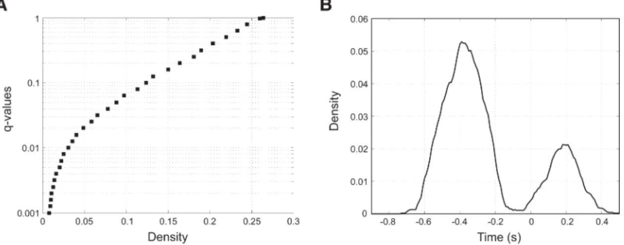
Figure 4

A

shows the FC network density D (the ratio between the number of

functional links and the number of possible connections) as a

function of threshold q-values. The density of the functional

net-work trivially increase as a function of the threshold; that is, the

more functional links, the higher is the density. The density

val-ues for significant q

⬍ 0.05 are ⬍10%, meaning that the

func-tional network is not dense, but sparse. We then computed the

density for each time slice of the FCD. Network density is

maxi-mal (⬃5%) ⬃0.4 s and then displays a second peak 0.2 after finger

movement (2% in density), as shown in

Figure 4

B.

Finally, to identify the most important brain regions in the

average SFL graph, we computed the strength S (sum of

func-tional links of a region), the eigenvector centrality EC, and the BC

at q

⬍ 0.05. The strength of a brain area is the simplest measure to

estimate the importance of a node in a network. A natural

exten-sion of strength centrality is eigenvector centrality EC and it

stands on the notion that a node is important if it is linked to by

other important nodes. In fact, a node receiving many links (i.e.,

high strength) does not necessarily have a high eigenvector

cen-trality because it may be linked to node with low strength.

There-fore, EC provides additional information because it computes the

centrality of a node as a function of the centralities of its

neigh-bors. Finally, the BC is equal to the number of shortest paths that

pass through a brain region. Therefore, a region with high BC has

the potential to play a key role in the network. Convergence of

Figure 3. SFL. A, Mean SFL connectivity matrix averaged over time. B, SFL time course averaged over pairs of areas. The threshold for significant SFL was equal to 2.43. Error bars indicate the 95% confidence interval.

these three metrics provides information about the importance

of different brain regions in the network.

Table 1

shows the brain regions sorted in a descending

order according to S, EC, and BC. The brain areas that

com-monly emerge as relevant across the three measures are the

dorsomedial and dorsolateral sensorimotor regions (Mdm,

Mdl, Sdm), in addition to dorsolateral premotor area (PMdl),

superior parietal regions (SPC, SPCm), and the caudomedial

visual cortex (VCcm).

Dynamic reconfiguration of FC subnetworks

To search for functional subnetworks generating the observe

dy-namics, we performed link community analysis. To do so, we first

computed the Pearson linear correlation between significant (at

q

⬍ 0.05) pairs of SFL time courses. Then, we found the optimal

subdivision of such link graph into communities of links using an

algorithm that attempts to optimize the “modularity” of a

parti-tion of the network, named the Louvain method (Blondel et al.,

2008). This approach provides a subdivision of nonoverlapping

communities by maximizing the number of within-group edges

and minimizing the number of between-group edges. Given that

community detection was performed on links, the detected

sub-networks represent link communities, in which individual brain

areas may participate in multiple overlapping networks. The

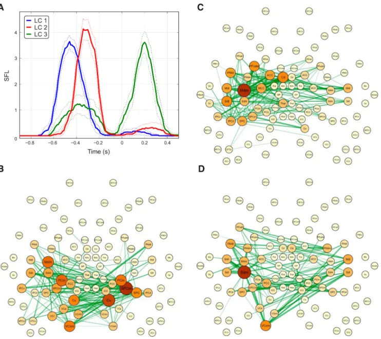
analysis revealed the presence of three link communities (Fig. 5).

The first link community (LC1) primarily included the visual and

superior and medial parietal regions bilaterally, in addition to the

left dorsomedial and dorsolateral sensorimotor regions (Fig. 5

B).

These brain regions form a FC subnetwork emerging

⬃0.5 s

be-fore finger movement, approximately corresponding to the

pro-cessing of the visual cue (Fig. 5

A). The second link community

(LC2) included the left dorsolateral and dorsomedial

sensorimo-tor regions and the dorsal frontoparietal network. Interestingly, it

included the middle and anterior cingulate cortices, the

dorso-medial prefrontal cortex, and the dorstal striatum in the caudate

nucleus (Fig. 5

C). LC2 emerged later during the trial and its

maximum of expansion occurred

⬃100–150 ms after LC1,

⫺0.35 s before movement. LC3 involved a larger brain network

involving the bilateral sensorimotor regions, the left

frontopari-etal network, and visual areas (Fig. 5

D). LC3 showed a strongest

peak after finger movement at 0.2 s, but displayed a peak at

⫺0.4

s. The only regions of the temporal lobe showing significant FC

were the superior and midtemporal cortices in the left

hemi-sphere. However, these regions displayed a relative weak strength

in the observed networks (Fig. 5

B–D). Overall, the link

commu-nity analyses allowed us to identify multiple and spatially

over-lapping FC patterns that evolve dynamically during the trial.

We can therefore depict the involvement of key brain regions

in a given link community such as the motor and premotor areas.

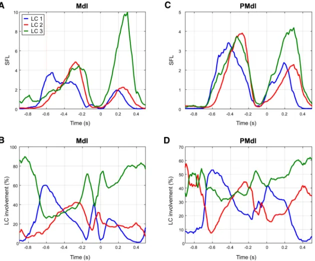
Figure 6

shows the contribution of the dorsolateral motor and

dorsal premotor areas, Mdl and PMdl, respectively, in the three

subnetworks as it unfolds over time. Around the presentation of

the visual stimulus, the Mdl primarily participates in the LC1,

which gradually declines over time (blue curve in

Fig. 6

A, B).

Then, its involvement in LC2 and LC3 increases in parallel, but

peaks earlier for LC2 (red curve in

Fig. 6

A, B) rather than for LC3

(green curve). These curves depict the dynamic reconfiguration

of the primary motor area from stimulus onset to motor output.

For the dorsolateral premotor cortex, its contribution peaking for

LC1, followed by LC3 and LC2 (Fig. 6

C,D), confirms that the

dynamic engagement in different subnetworks occurs over a

short timescale.

Finally, to quantify the dynamics of reconfiguration among

the three functional subnetworks, we inferred the evolution of

network “flexibility” (following the same ideas developed in

Braun et al., 2015). We defined the flexibility of a given brain

region as the entropy associated with the probabilities of

involve-ment in the three LCs (shown in

Fig. 6

B, D, for Mdl and PMdl,

respectively). Accordingly, node flexibility is maximal for nodes

participating with equal probability in the different LCs and

min-imal for nodes participating in a single LC.

Figure 7

A shows the

mean dynamics of network flexibility averaged over nodes.

Inter-estingly, it reconfiguration shows a single peak occurring at

⬃0.4

s before finger movement, which corresponds to the moment

Figure 4. Graph theoretical measures. A, Dependence between threshold values (q-values) and FC density. B, Temporal evolution of density D at q⫽ 0.05.

Table 1. Graph theoretical measures

S EC BC

Value Region Value Region Value Region 7.39 Mdm 6.84 Mdm 16.25 Sdm 6.28 Sdm 6.42 Sdm 13.68 Mdm 4.64 Sdl 5.73 Sdl 9.98 Cu 3.88 PMdl 4.98 Mdl 9.52 VCcm 3.75 VCcm 4.37 PMdl 6.19 Sdl 3.70 Mdl 3.82 Cd 5.81 Mdl 3.34 SPC 3.56 VCcm 4.80 PMdl 3.25 SPCm 3.37 SPCm 4.46 IPCd 3.20 Cu 3.20 PFcdm 3.83 SPC 3.13 Cd 3.05 PCC 3.41 SPCm

when the three LCs overlap more strongly in time and space.

Figure 7

B shows the mean flexibility averaged over time for the

first five strongest brain regions. The parietal regions (SPC, PCm,

and PPC) display the largest flexibility, together with the dorsal

premotor cortex.

Control analyses and intracranial SEEG validation

The interpretation of FC measures from noninvasive techniques

such as EEG and MEG may suffer limitations, among which

vol-ume conduction and leakage are potential confounds (Bastos and

Schoffelen, 2015). We performed a series of control analyses to

assess the influence of such confounds.

First, we studied the relation between the mean SLF for two

subcortical regions displaying a significant increase in HGA and

FC with cortical regions as a function of their respective distance

to cortical regions. The rationale was to investigate whether

vol-ume conduction and leakage effects could have produced the

observed HGA modulations in subcortical regions and the FC

patterns between deep sources, such as the thalamus and caudate

nucleus and cortical areas.

Figure 8

shows that a clear relation

between distance and FC measures (as assessed through the mean

SFL) is lacking for the thalamus (Fig. 8

A) and for the caudate

nucleus (Fig. 8

B).

Second, we investigated the dipole orientation of all sources

within the thalamus and caudate nucleus. The rationale was that

differences in dipole orientation of nearby regions may suggest

that the estimated HGAs originate from spatially separable brain

structures. We computed the average dipole orientation both for

the thalamus and caudate nucleus. Then, we compared the

aver-age dipole orientations by means of the normalized inner

prod-uct. This measure equals one for identically oriented dipoles

minus one for dipoles pointing in opposite directions and zero

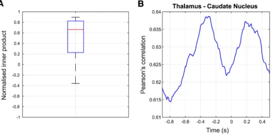
for orthogonal dipoles. The boxplot displayed in

Figure 9

A

de-picts the distribution of normalized inner products between the

thalamus and caudate nucleus across participants. The values of

normalized inner products span a broad range from

⫺0.45 to

Figure 5. FCD. A, Time course of the average SFL for the three identified LCs. Error bars indicate the 95% confidence interval. Spatial patterns for the three LCs are displayed in B–D. The thickness of the green links is proportional to the time-averaged SFL between areas and the color and size of nodes are proportional to the mean SFL between each area and the rest of the network (i.e., the weight).

0.85, with median value around 0.65. Extremely high values of

raw correlation coefficient between subcortical HGAs would also

suggest strong leakage effects. We thus plotted the Pearson

cor-relation coefficient between the HGA at the thalamus and

cau-date nucleus, averaged over sessions and participants (Fig. 9

B).

The value in the prestimulus interval (i.e.,

⬃⫺0.8 s before finger

movement) was 0.615. The corresponding coefficient of

determi-nation R

_{was 37,8% (i.e., R}

_{⫽ 0.615 ⫻ 0.615 ⫽ 0.3782) and}

equals the proportion of the variance in HGA shared by the

thal-amus and caudate nucleus.

Finally, to assess the relevance of cortical HGA modulations,

we asked three patients candidate for surgical treatment of

drug-resistant epilepsy to perform the same visuomotor task while

recording SEEG in multiple brain areas. HGA from intracranial

recordings in epileptic patients is largely exploited for cognitive

mapping and represents an optimal opportunity to validate MEG

results. Results from single-patient SEEG cannot be taken as

rep-resentative of the population, contrary to group-level MEG

re-sults. In fact, we cannot exclude that across-subject variability is

due to either physiological and/or pathological factors. However,

SEEG data provide direct measures of intracranial HGA, free

from alteration due to volume conduction or limitation of source

imaging tools. Therefore, they provide important additional

ev-idence to support the significance of the MEG results.

Electrodes were localized by combing postimplant CT scans

with presurgical anatomical MRI scans and were labeled

accord-ing to MarsAtlas (see Materials and Methods). Saccord-ingle-trial HGA

for each labeled brain region of MarsAtlas was defined as the

mean z-transformed power values averaged across all electrodes

within the same region. To increase the local specificity of SEEG

recordings, bipolar derivations were performed among adjacent

contacts. Statistical analyses were performed separately for each

Figure 6. Exemplar evolution for the dorsolateral motor (A, C) and premotor (B, D) areas. A and B show the involvement of Mdl and PMdl in the three LCs, respectively. C and D depict the involvement in percentage value.

Figure 7. Flexibility analysis. A, Mean evolution of network flexibility (shaded area repre-sents the SD). B, Areal flexibility for the five most representative brain regions.

patient. Twelve brain areas across the three patients were found

to display a significant increase in HGA (Table 2; q

⬍ 0.05). These

included the dorsomedial and dorsolateral motor cortex, the

dor-solateral somatosensory region, and the dorsal frontoparietal

network (SPC, SPCm, PMdl, and PMdm). In patient 2, the

ven-tral portions of the motor and premotor areas were significantly

active. Note that the SEEG implant did not cover the entire brain,

but selected regions in the frontoparietal network.

We then compared the average time course of single-patient

HGA modulations with those from the MEG group-level analyses

(Fig. 10). Seven of 12 regions displayed a strong (larger than 0.65)

linear correlation between the group-level MEG results and the

single-patient SEEG time courses. The most striking similarity

was observed for brain regions of the sensorimotor cortices and

the dorsal frontoparietal network. Overall, these results confirm

that the increase in HGA observed in the MEG data over

senso-rimotor cortices and the dorsal frontoparietal network results

from area-specific increases in HGA, rather than by leakage from

nearby regions displaying a strong response.

Discussion

Brain network and interactions of visuomotor mapping

Previous analyses of arbitrary visuomotor-related FC have shown

that parietal areas play a driving role in the network, whereas

premotor areas act as relays from parietal to medial prefrontal

cortices, which participate as receivers (Brovelli et al., 2015). Such

an approach, however, neither considered the time-evolving

na-ture of FC patterns nor analyzed the involvement of subcortical

areas. Our whole-brain and time-dependent brain connectivity

Figure 8. Relation between mean FC and distance for the thalamus (A) and caudate nucleus (B). Each dot corresponds to a brain area displaying significant FC with the seed regions.

Figure 9. Distribution of normalized inner products between the average dipole orientations of the left thalamus and caudate nucleus across participants (A). The boxplot depicts extreme values (whiskers), first and third quartile (box) and median (red line). B, Time course of mean correlation coefficient.

Table 2. SEEG activations

Parcel name Peak p-value Peak t-value Peak

time (s) Time interval (s)

Patient no. L Mdm 3.42E-20 11.43 ⫺0.175 ⫺0.28 0.125 1 R SPC 8.76E-20 11.15 ⫺0.22 ⫺0.44 0.2 3 R PMdm 1.41E-17 10.27 ⫺0.34 ⫺0.62 ⫺0.06 2 L PMdm 5.65E-17 10 ⫺0.29 ⫺0.455 0.155 1 R SPCm 4.85E-17 9.96 ⫺0.045 ⫺0.275 0.05 3 L Mdl 2.21E-15 9.29 ⫺0.435 ⫺0.555 ⫺0.315 1 R Mdl 1.52E-14 8.92 ⫺0.165 ⫺0.39 0.055 2 R PMrv 6.70E-14 8.63 ⫺0.145 ⫺0.5 0.155 2 L Sdl 1.29E-12 8.05 0.045 ⫺0.225 0.26 1 R IPCd 1.69E-12 7.96 ⫺0.28 ⫺0.415 ⫺0.135 3 L PMdl 4.22E-12 7.82 ⫺0.315 ⫺0.45 ⫺0.185 1 R Mv 2.78E-11 7.44 ⫺0.02 ⫺0.44 0.18 2 R Mdl 9.89E-08 5.72 ⫺0.475 ⫺0.51 ⫺0.4 2

analyses showed that visuomotor mapping resides in three

dis-tinct and partly overlapping subnetworks with time-evolving

cortico-cortical and cortico-subcortical interactions.

Approxi-mately 0.5 s before finger movement, visual and parietal regions

coordinate with sensorimotor and premotor areas (LC1 in

Fig.

5

B; blue curve in

Fig. 5

A). Subsequently, the sensorimotor

gions, the dorsal frontoparietal circuit, the medial prefrontal

re-gions, the basal ganglia, and the thalamus (LC2 in

Fig. 5

C)

dominated the FC pattern. The dorsal frontoparietal circuit,

known to support visuomotor transformations and goal-directed

attentional processes (Wise et al., 1996;

Wise and Murray, 2000;

Corbetta and Shulman, 2002;

Culham and Valyear, 2006), is

tightly coupled with the sensorimotor and associative

frontos-triatal circuit for a brief period around 0.35 s before action (red

curve in

Fig. 5

A). This FC network includes medial prefrontal

areas, such as the dorsomedial prefrontal cortex (PFCdm),

mid-cingulate cortex (MCC), anterior mid-cingulate cortex (ACC) and

rostro-medial prefrontal (PFrm), with a strongest increase in

HGA in the MCC and PFCdm (Fig. 2). The involvement of

medial prefrontal areas may correspond to the activation of

visuomotor-related neural populations of the rostral cingulate

zone (RCZ), a key node of the human motor system (Picard and

Strick, 1996;

Amiez and Petrides, 2014). At the subcortical level,

the dorsal striatum (caudate nucleus and putamen), globus

pal-lidus and thalamus displayed the strongest HGA in the

hemi-sphere contralateral to the motor response (Fig. 2). Indeed,

intracranial recordings from patients with motor disorders have

described HGA in the subthalamic nucleus (Amirnovin et al.,

2004;

Alegre et al., 2005;

Androulidakis et al., 2007;

Lalo et al.,

2008), globus pallidus (Tsang et al., 2012) and thalamus (Bru¨cke

et al., 2013) during different types of motor behaviors.

High-gamma oscillatory activity in the subthalamic nucleus (STN) and

globus pallidus (GPi) has been found to be coherent with cortical

activity during voluntary movement (Cassidy et al., 2002;

Brown,

2003). Granger causality analysis also showed that STN drives

activity in M1 (Litvak et al., 2012), thus suggesting that HGA in

motor areas is due to propagating activity from the basal ganglia

through the thalamus (Bru¨cke et al., 2013). Our results showed

that the caudate nucleus and thalamus are coupled with the

sen-sorimotor cortex and the dorsal frontoparietal networks (LC2 in

Fig. 5

C), thus confirming a dynamic coordination between

cor-tical and subcorcor-tical regions also during visuomotor behaviors

most prominently during the planning phase before movement

initiation.

Several lines of evidence suggest that the reported subcortical

activations are primarily local, rather than due to leakage from

cortical areas. First, we observed that the putamen significantly

activated only in the left hemisphere, whereas the thalamus was

activated bilaterally (Fig. 2). If the bilateral activation in the

thal-amus were due to leakage from cortical areas, we would have

expected a bilateral activation also in the putamen, given that the

thalamus is deeper than the putamen. Second, no significant

correlation was found between the SFL and distance for the

thal-amus and caudate nucleus (Fig. 8). Third, the average dipole

orientation for the thalamus and caudate nucleus are significantly

different (i.e., the normalized inner product is

⬍ 1) and the

dis-tribution of values covers a wide range from

⫺0.45 to ⬃0.85. This

suggests that the thalamus and caudate nucleus lack a systematic

similarity in dipole orientation (Fig. 9

A). Fourth, the mean

Pear-son correlation values and the corresponding coefficient of

determination do not saturate at high values and show a

modu-lation similar to the average time course of FCD (Fig. 9

B). This

suggests a lack of strong covariance, as would be expected if

leak-age effects were dominating.

Nevertheless, we cannot a priori exclude that the observed

subcortical increases in HGA and FC patterns may be due to

complex configurations of cortical activations. Indeed, we

sug-gest that HGA estimation at subcortical areas and FC analysis

should not be performed blindly. Rather, the analysis of raw

cor-relations and dipole orientations provide important insight into

the origin of the results. Experimentally, simultaneous MEG and

subcortical measures of HGA from intracranial recordings would

be required to confirm or disprove the ability of MEG to capture

subcortical HGA and FC.

Overall, our result suggests that the basal ganglia form a

dy-namic functional network, which may allow the coordination

within and across different processing streams in the basal ganglia

(Brown, 2003) and facilitate motor output (Cheyne and Ferrari,

2013). The involvement of sensorimotor and associative

fronto-striatal circuits, classically thought to be involved in habits (Yin

and Knowlton, 2006;

Graybiel, 2008;

Ashby et al., 2010), also

suggests that performance of arbitrary visuomotor mappings can

be viewed as a form of acquainted instrumental behavior

(Brov-elli et al., 2015), the gradual consolidation of which would lead to

Figure 10. SEEG validation of HGA modulations. Comparison between SEEG single-subjects t-value for HGA (blue) and group-level MEG results (red curves). Subject number, brain areas, and the correlation coefficient between the curves are indicated on the top of each panel.