Contact fatigue : life prediction and palliatives

(1)

Contact Fatigue: Life Prediction and Palliatives

by

Brett P. Conner

B.S., University of Missouri-Columbia (1998)

S.M., Massachusetts Institute of Technology (2000)

Submitted to the Department of Materials Science and Engineering

in partial fulfillment of the requirements for the degree of

Doctor of Philosophy

at the

MASSACHUSETTS INSTITUTE OF TECHNOLOGY

September 2002

c

° 2002 Massachusetts Institute of Technology. All rights reserved.

The author hereby grants to Massachusetts Institute of Technology permission to

reproduce and

to distribute copies of this thesis document in whole or in part.

Signature of Author . . . .

Department of Materials Science and Engineering

20 August 2002

Certified by . . . .

Subra Suresh

R. P. Simmons Professor and Head, Department of Materials Science and Engineering

Thesis Supervisor

Accepted by. . . .

Harry L. Tuller

(2)

Contact Fatigue: Life Prediction and Palliatives

by

Brett P. Conner

Submitted to the Department of Materials Science and Engineering on 20 August 2002, in partial fulfillment of the

requirements for the degree of Doctor of Philosophy

Abstract

Fretting fatigue is defined as damage resulting from small magnitude (0.5-50 microns) dis-placement between contacting bodies where at least one of the bodies has an applied bulk stress. The applicability and limits of a fracture mechanics based life prediction is explored. Comparisons are made against highly controlled experiments and less controlled but more re-alistic experiments using a novel dovetail attachment fixture. Surface engineering approaches are examined from a mechanics perspective. Using a new tool, depth sensing indentation, the mechanical properties of an aluminum bronze coating are determined. Fretting fatigue experi-ments are performed on specimens coated with aluminum bronze and on specimens treated with low plasticity burnishing. Low plasticity burnishing is a new method of introducing beneficial compressive residual stresses without significant cold work at the surface. A mechanics based approach to the selection of palliatives is addressed.

Thesis Supervisor: Subra Suresh

(3)

List of Figures

1-1 a.) Fretting wear involves small cyclic displacements as a result of contact alone. b.) Fretting fatigue is fretting in the presence of a bulk fatigue load. Fatigue cracks can develop and will propagate if the bulk load is suﬃciently large. . . 15 1-2 h is the amount of overlap if two bodies can freely penetrate. After Hills and

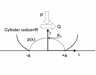
Nowell 1994. . . 21 1-3 Application of a normal load, P , to a cylindrical contact produces a parabolic

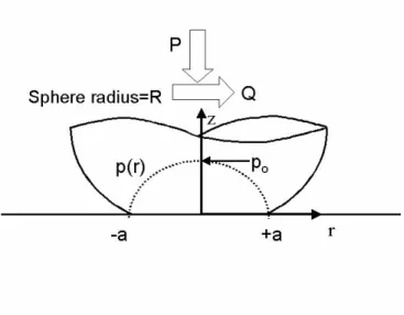
pressure distribution, p(x) which goes to zero at a and has a maximum at x = 0. 24 1-4 A top-down view of the contact between spheres (or a sphere and a flat). The

geometry of the contact patch is a circle of radius a. It should be noted that application of a load tangent to the contact is typically in the x-direction. . . 25 1-5 Application of a normal load, P , to the spherical contact results in a parabolic

pressure distribution, p(r), with a pressure of zero at ±a and a maximum pressure at x = 0. . . 26 1-6 A schematic of the shear traction, q(r), and the pressure traction, p(r), for a

spherical contact. . . 27 1-7 If Q < f P , slip will be confined only to the outer regions of contact, while an

adhered region, referred to as the stick zone, will develop at the center of contact. 28 1-8 Normalized pressure and shear tractions shown for a cylinder with Q/fP=0.8. . . 28 1-9 Adhesive energy between the two bodies results in an increase in contact radius

(7)

1-10 The solid line represents the contact pressure including adhesion. The first dashed line shows the bounded pressure without adhesion and the second (on the right) shows square root pressure. . . 31 1-11 The normalized pressure distribution for a flat punch of length 2a with rounded

corners resulting in contact length 2b. Various values a/b are shown. . . 32 1-12 Normalized shear tractions are shown for values of a/b and Q/fP of 0.8 . . . . 34 1-13 The pressure and shear tractions are shown for two extremes of the flat punch

with rounded corners: a/b=0.9 and a/b=0.0 for Q/fP =0.8. . . 35 2-1 A photograph of the MIT fretting fatigue fixture. The extensometer can be

clearly seen to the left of the specimen. The width of the bar specimen is 4.74 mm. . . 39 2-2 A schematic of the MIT fretting fatigue fixture showing the location of load cells,

applied loads and supports. . . 39 2-3 The first series of experiments varied the maximum bulk stress applied in each

test for several contact conditions. The results are compared with plain fatigue data from Bellows et al. [58]. . . 41 2-4 Keeping Q fixed at 17 N, P is varied. The maximum bulk stress is 300 MPa.

Notice the eﬀect of increasing the pad radius from 12.7 mm to 25.4 mm. . . 42 2-5 The tangential load is varied for each test while P is held at 50 N. Again, a

decrease in the pad radius results in a decrease in the fretting fatigue life at a given Q/P . . . 43 2-6 A fretting fatigue scar for a specimen after 10,000,000 cycles (P =24 N, Q=17

N, pad radius of 25.4 mm and max bulk stress of 300 MPa). A crack developed but did not propagate to failure. . . 45 2-7 In the sphere-on-flat experiments, cracks would initiate only on the side closest

to the actuator. . . 45 3-1 A photograph of the dovetail fixture and specimen. . . 47 3-2 A schematic of the dovetail fretting fatigue fixture. . . 48 3-3 A large crack developed near the maximum edge of contact in Specimen # T2. . 49

(8)

3-4 A section taken from the scar in the previous figure shows that cracks have developed in the slip regions near both edges of maximum contact length. The largest crack is the same crack visible in the previous figure. . . 50 3-5 The global mesh for the dovetail finite element model. Notice that the mesh in

both the specimen and the fixture becomes refined closer to the interface. . . 53 3-6 In the case of the short flat contact geometry, nearly 130 elements are located

near the contact region. . . 53 3-7 The calculated hystersis loop over two cycles of loading for several values of the

coeﬃcient of friction. . . 54 3-8 The strain versus load response measured at the strain gauge compared to the

calculated response from the model. . . 55 3-9 A schematic of the boundary conditions and loads involved in the dovetail model. 56 3-10 A plot of the pressure for a cylindrical contact of a dovetail specimen loaded

at P =1900 N. Notice the large scatter in pressure values near the maximum contact pressure. . . 58 3-11 The evolution of shear tractions from 5% of maximum load to 100% of maximum

load for a dovetail specimen contacted by a cylindrical pad. f =0.8. . . 59 4-1 A schematic of the flat-on-flat fixture developed at AFRL. . . 61 4-2 Two fretting cracks initiated (location shown by arrows) and linked. . . 63 4-3 Debris flows into a crack in the slip region of a dovetail specimen. The contact

pad was a short flat with taper. . . 64 4-4 A crack from a wear crater grows into an asperity. . . 65 4-5 SEM image of surface damage showing delamination and the formation of small

notches developing into cracks (P =50 N, Q=27.5 N, N =300,000 cycles, σaxial=270 MPa, R=0.1, r =12.7 mm). . . 65 4-6 A small crack (0.5 µm) growing out of a notch. This is one of the notches shown

in the above photo. . . 66 4-7 Wear debris fill fretting cracks. . . 66 4-8 Small fretting fatigue crack filled with wear debris. . . 67

(9)

4-9 a.) A small crack has developed near the edge of contact. b.) Oxides developed by wear enter the crack as it is opened by contact and bulk tensile stresses. Either one of two eﬀects occur: c.) the crack jumps ahead of the wedge during compressive loading or d.) crack growth is slowed by closure. . . 68 4-10 A schematic of the dependence of the fatigue life and the wear volume loss (W )

on the fretting displacement slip amplitude. The highlighted region is the region where wear debris most impacts fatigue life. . . 70 4-11 The coeﬃcient of friction is initially constant in across the contact patch (shown

here to be circular). Over n cycles, the coeﬃcient of friction will increase in the slip region as a result of wear. Therefore, the radius of stick will also increase. 72 4-12 f versus fn for selected values of Q/P . . . 74 4-13 The relationship between f and fn is diﬀerent for spherical and cylindrical

con-tacts. The dashed lines represent the cylindrical contact. . . 75 4-14 A plot of f (the vertical axis) and fn (the horizontal axis) for w=0, 0.1 and 1.

As w increases from zero, so does the value of f with respect to fn. . . 79 4-15 Experimentally measuring the coeﬃcient of friction in the slip zone over n cycles. 80 5-1 Aspects of the rigid punch contact problem in a.) can be equivalent to those of

the double edge cracked specimen in b.) . . . 84 5-2 The normal traction, p, in the punch problem is square root singular in the

asymptotic limit as one approaches the edge of contact. . . 85 5-3 For a contact without adhesion, the pressure is bounded and zero at the edge

of contact ±a. However, the presence of adhesion would cause the pressure to become singular at the new edge of contact, ±amax, for strongly adhered contacts or at the stick zone boundary, ±c, for weakly adhered contacts. . . 85 5-4 A schematic of a kinked crack. The mechanics of a kinked crack will be used to

determine crack orientation and early crack growth of fretting fatigue cracks. . . 87 5-5 ∆k1 is plotted versus number of cycles to failure for experiments where P is

varied while Q is held fixed at 17 N and the maximum bulk stress is 300 MPa. 92 5-6 ∆k1 is plotted versus number of cycles to failure for experiments where Q is

(10)

5-7 A plot comparing the experimental life versus the predicted life using the fracture mechanics methodology. Experiments from several geometries and fixtures are shown. . . 95 5-8 Multiple fretting fatigue cracks emerge from the contact surface (at the bottom

of the micrograph). The dominant crack is oriented at a 48.7 degree angle to the surface and turns normal to the bulk stress by 17.6 microns. . . 96 5-9 ∆k1 versus number of cycles to failure for cylindrical contact (Al 4%wt Cu) and

R=-1. . . 97 6-1 A low magnification composite SEM image of the fretting scar of a coated

spec-imen after a crack has developed and propagated. . . 102 6-2 a.) A 3-D surface profile showing material removal to a depth of 29 microns

in a small section of the slip zone from a coated specimen. b.) An uncoated specimen showing significantly less material removed in the slip region. c.) and d.) show 2-D surface profiles taken in a.) and b.) respectively. . . 103 6-3 Transitioning the crack analogue to a coated body with coating thickness h via

the complex stress intensity factor K. . . 105 6-4 A schematic of a P-h curve. . . 106 6-5 A micrograph looking down into a indentation into the coating. Note the small

dents and particles on the surface. . . 108 6-6 A photograph of an LPB treated specimen in the dovetail fixture. Notice the

polished appearance of the specimen regions near the contact pad. This is a result of the contact pressure from the rolling sphere. . . 110 6-7 The maximum load for failure at 106 _{cycles (R=0.1)for baseline specimens and}

LPB treated specimens. . . 111 6-8 The number of cycles to failure for an 18.3 kN maximum load (R=0.1).

Signif-icant improvement for the LPB treated specimen. . . 112 6-9 X-ray diﬀraction measurements of the burnishing induced residual stresses under

the fretting fatigue scar and away from. . . 113 6-10 X-ray diﬀraction measurements of the burnishing induced % cold work

(11)

6-11 A plot showing the stress intensity factor as a function of crack length for a crack at the edge of contact and normal to the surface. 3 diﬀerent test conditions are considered corresponding to an untreated specimen at baseline loads, a specimen treated with LPB at baseline loads, and specimen treated with LPB with a 50% increase in maximum load resulting in failure at 106 cycles. . . 117

(12)

List of Tables

2.1 A list of some of the mechanical properties of the Ti-6Al-4V alloy. TS=tensile strength. TF=true fracture stress. RA=reduction in area at fracture. SR=strain

rate . . . 40

2.2 Contact radii and pressures for Ti-6Al-4V pads pressed into a flat surface at 50 N. 41 3.1 Experimental results from dovetail fretting tests. Loads in kN; sg=strain gauge; vm=video strain mapping. . . 51

3.2 Measurements of fretting fatigue scars . . . 51

3.3 Elastic properties of materials used in finite element model of the dovetail. . . 52

3.4 Loads as determined via FEM. LPB is low plasticity burnishing and will be described in Chapter 6. . . 57

3.5 Loads as determined via FEM compared with the upper bound when f=0. . . 58

4.1 Experimental results for Ti-6Al-4V on Ti-6Al-4V spherical contact . . . 79

5.1 Conditions for experiments reported by Hutson et al. . . 91

5.2 Predictions for stresses in the x-direction for failure at 1e7 cycles. . . 91

5.3 Some mechanical properties of the alloys used in the selected fretting fatigue tests 91 5.4 Stress intensity factors and crack orientation angles for the dovetail experiments. 94 5.5 Fatigue life predictions for conditions used in each of the dovetail experiments. ro=runout . . . 94

(13)

6.2 Complex K for the experimental conditions listed above. It is assumed that the Poisson’s ratio of the substrate and the coating are equal. n/f means no failure. . 105 6.3 Experimental results for fretting fatigue of LPB treated specimens . . . 111 6.4 Stress intensity factors and crack orientation angles for the LPB treated dovetail

experiments. . . 116 6.5 Fatigue life predictions for conditions used in each of the LPB dovetail

(14)

Chapter 1

Introduction

1.1 Background

Contact fatigue can be defined as damage resulting from cyclic relative motion between two surfaces. As a result, component service life may be reduced and maintenance costs could increase as inspections, repairs and palliatives may be required. The list of engineering systems aﬀected by contact fatigue is long and stretches across the engineering spectrum including aerospace systems, micromechanical devices, railroad tracks, chain links, ball bearings, and biomedical implants [1, 2, 3, 4].

A particularly damaging form of contact fatigue is fretting fatigue. Fretting wear is defined as cyclical small displacements between two bodies in contact. In fretting fatigue, one or both of the bodies also have an applied cyclical bulk stress. The fretting is then accompanied with fatigue damage and if the cyclic bulk load is suﬃciently large, fatigue cracks may propagate to failure.

There are competing demands on the engineer who faces contact fatigue. The design engi-neer desires guidelines to prevent or minimize contact fatigue. The maintenance engiengi-neer wants reliable service life predictions with room for safety, yet predictions that are less conservative result in more economical ownership costs. Before these demands can be met, the materials science and mechanics of contact fatigue must be more fully understood.

(15)

Figure 1-1: a.) Fretting wear involves small cyclic displacements as a result of contact alone. b.) Fretting fatigue is fretting in the presence of a bulk fatigue load. Fatigue cracks can develop and will propagate if the bulk load is suﬃciently large.

1.1.1 Historical perspectives on fretting fatigue

Much of the eﬀort in contact fatigue research has been focused on fretting fatigue for two primary reasons. First, fretting fatigue is encountered in many engineering systems. Second, all the major variables can be obtained experimentally including a bounded displacement.

One of the earliest articles on fretting fatigue was that of Eden et al. who in 1911 noted that oxides formed in the grips of a tensile fatigue specimen [5]. Early fretting fatigue developments included linking oxide formation to tangential contact loading [6] and discovery that fretting fatigue reduces the fatigue strength [7].

In the 1960’s, some of the more common experimental methods were developed. The first was the bridge pad apparatus which gives a constant stress distribution equal to the normal load divided by the contact area. This was soon followed by the development of a fretting fatigue fixture that held a cylindrical pad. The primary advantage of this geometry is that analytical solutions exist for the stresses under a cylindrical pad [8]. These will be discussed in detail later.

The field of contact mechanics provided the necessary tools to determine stresses and dis-placements under fretting contacts. Hertz solved the boundary value problem to obtain the

(16)

contact pressure underneath cylindrical and spherical indenters [9]. Cattaneo [10], and later Mindlin [11], found the tangential tractions underneath spheres in partial-slip conditions; a useful development for the study of fretting fatigue. The tractions underneath a partial-slip cylindrical contact can be found in detail in [12].

The application of fracture mechanics in fretting fatigue was first considered by Endo and Goto [13] then Edwards [14]. Accounting for the stress gradients resulting from contact requires application of a weight function such as in [15]. Another approach is that of Hills and Nowell who suggest the use of a distribution of hypothetical dislocations to model the stress field and boundary conditions of the fretting fatigue crack [16]. One can also use fracture mechanics to determine total life by assuming that all of the life is propagation [17]. In this method, an eﬀective initial flaw size (non-physical) is assumed based on a large body of experimental data.

Beyond stresses and displacements, other damage mechanisms were considered by researchers. The eﬀect of adhesion on fretting fatigue was first approached by Godfrey [18], and later by Bethune and Waterhouse [19]. Since friction can increase temperatures, several researchers considered experimental measurements or theoretical predictions to determine the magnitude of temperature increase as a result of fretting and what, if any, material damage may result [20, 21, 22].

1.1.2 Recent developments

While the study of the eﬀects of contact fatigue can be traced back to the failure analysis of railroad tracks in the late 1800’s, remarkable headway has occurred in the last ten to twenty years.

One of the major recent eﬀorts in fretting fatigue centered around the progression of wear damage and its impact on fretting fatigue life. Most of this research was performed by research teams in France. Fretting maps were developed from a large quantity of experiments showing regimes of no slip, partial-slip or stick-slip, mixed slip and gross slip plotted in an analytical space bounded by the applied normal load and the displacement [23]. In general, the fatigue life decreased significantly during partial-slip conditions as opposed to gross-slip conditions. However, many experiments begin with gross-slip that eventually becomes stick-slip after several hundreds or thousands of cycles as a result of wear damage. This evolution of the coeﬃcient

(17)

of friction was qualitatively demonstrated through plotting the tangential load/displacement hysteresis loops over the entire life of the experiment. Hills, Nowell and Sackfield analytically determined the evolution of the coeﬃcient of friction for a Hertzian contact [24].

At Oxford, extensive eﬀort was placed into developing an experimental apparatus to mea-sure and control all fretting fatigue variables [25]. Upon obtaining these variables, one could use the experimental results for validation of fretting fatigue models. It was determined that the common bridge pad fretting fatigue apparatus did not permit partial slip conditions since a stick region was not permissible under a flat surface [26]. Simple non-conforming Hertzian contacts and partially conforming contacts such as flat punches with rounded corners permitted experiments with partial slip contact conditions. Such an approach required careful develop-ment of fretting fatigue experidevelop-mental fixtures particularly to quantify the tangential loading and the displacement. Key features included interchangeable pads and specimens, load cells to quantify tangential loads, and extensometers to measure displacements.

Ruiz, also at Oxford, developed a fretting fatigue damage parameter based on work-energy principles [27]. He realized that the work performed in fretting is the area of the local shear times the local displacement (both shear and displacement vary over the interface) or τ δ. This parameter reasonably predicted the location of fretting fatigue cracks in dovetails but not so for other geometries. As a result, Ruiz and Chen empirically added the maximum normal stress, στ δ, and showed reasonable nucleation location for the sphere-on-flat geometry [28]. Thus, a unique fretting fatigue parameter has been developed but without a fully physical basis.

In the area of contact fatigue modelling, several recent advances should be noted. One was Ciaverella’s development of a generalized Cattaneo-Mindlin analytical solution of contact pressure distributions[29]. This enabled researchers and engineers to determine the surface tractions for almost any contact geometry. In particular, the rounded punch contact problem was examined in detail because of its relevance to the dovetail attachment fatigue [30, 31].

Fretting fatigue at lap joints in aging aircraft prompted research into rivet geometries [32]. Temperature gradients were measured experimentally to validate numerical contact modelling, but the temperature increases in aluminum alloys proved to be on the order of 1 K [33]. Even-tually, some of this work was folded into research sponsored by the U. S. Air Force on fretting fatigue in gas turbine engines (to be discussed in the next section). This led to numerical

(18)

integration of closed-form singular integral contact equations [34]. This methodology rapidly generated solutions for the contact pressure, shear tractions and resultant stresses.

At MIT, a fretting fatigue apparatus was developed that was very similar to the one devel-oped at Oxford [35, 36]. This enabled a wide range of loading conditions and spherical pad radii to be examined using pads and specimens made of Al 7075 [36] and Ti-6Al-4V [37]. The normal load, tangential load, bulk stresses and pad radii are known for each test, so the results are readily available for model validation.

The MIT research group also developed several novel approaches to life prediction. De-parting from the stress-at-a-point approaches found in the literature [38, 39], Giannakopoulos, Lindley and Suresh proposed a method where aspects of contact mechanics can be described with fracture mechanics via analogy if appropriate [40]. This method opened new doors to crack nucleation predictions (“go-or-no-go”) and total life prediction. This methodology was extended to strong and weakly adhered contacts [41] as well as nearly-singular flat contacts [42]. Chambon compared experimental results and total life predictions from these models [43] while Kirkpatrick developed a theoretical approach to determining the depth necessary to peen without losing residual stresses as a result of yielding from the contact stresses [44]. Further details of the MIT experimental fixture and experiments is given below. This thesis builds on this foundation laid by these researchers at MIT.

1.2 Contact fatigue in aerospace materials

One of the primary motivations for this research is the role of contact fatigue in applications of aerospace materials. The demands placed on an aircraft structure are extensive. Mechanical and thermal loads can be extreme while density must be relatively light to reduce overall structure weight. An aircraft is subject to cyclic loading through wing loading, atmospheric turbulence, and cabin pressurization. The propulsion and hydraulic systems also experience cyclic loading. In the early to mid 1990’s, much research was focused on the problem of contact fatigue in rivet joints of aging aircraft. Common materials used in lap joints are the aviation aluminum alloys (2xxx or 7xxx series alloys) [32, 45]. During the mid 1990’s, the U. S. Air Force became concerned about dovetail joints in gas turbine engines. As a

(19)

result of these problems, the U. S. Air Force funded a National Turbine High Cycle Fatigue Program. This program was an eﬀort by government agencies, industry and universities to research the mechanics, life-prediction methods and palliatives for high cycle fatigue including contact fatigue. Estimates by the U. S. Air Force show that one in six of all in-service high cycle fatigue related engine mishaps were the result of fretting and galling [46]. As a result, inspections and regular maintenance procedures are performed in order to prevent catastrophic in-flight failures. An estimated $20 million is spent annually on these preventative measures [46]. Increased turbine maintenance also results in higher operating costs and lower mission availability. The seriousness of the contact fatigue problem is captured in this statement from a failure investigation.

”While a fighter was taxiing for takeoﬀ, a sudden “bang” was heard, the aero-engine vibrated violently and the rotational velocity declined. The fire warning light came on. The pilot immediately stopped the process of takeoﬀ and quickly left the fighter. Then the fighter caught fire. After field investigation, it was con-cluded that the accident resulted from the fracture failures of rotor blade and disk in the first stage compressor.” [47]

The common material used in the manufacturing of compressor blades and disks is Ti-6Al-4V or a variant of that alloy. Thus, this material will be the primary focus of the experiments in this thesis.

Contact fatigue plagues commercial aviation just as it does military aircraft. In 2001, an Emirates Air 777 was forced to abort takeoﬀ because of a fretting fatigue failure that liberated a fan blade that destroyed the engine. This incident prompted Rolls Royce to examine their contact fatigue palliatives to find one that could oﬀer more protection [48]. Obviously, the concern over safety increases by several orders of magnitude for a commercial aircraft, and there is still the economic cost of excessive maintenance and inspections.

It should be noted that space systems are also aﬀected by contact fatigue [49]. Contact damage (not necessarily fatigue) has eﬀected several prominent orbital missions including a gear failure on Sputnik, the fatal parachute failure of cosmonaut V. M. Kormarov, a docking failure on Salyut/Soyuz-10 mission [50], a stuck antenna on the Galileo space probe, and stick-slip

(20)

fatigue on the space shuttle’s orbital quick check values for the orbital maneuvering engines [51]. Ground testing revealed potential contact damage problems on the beta gimbal joints for the International Space Station [51]. The space environment produces unique problems such as vacuum and extreme temperature fluctuations for Earth orbiting spacecraft. The absence of an oxygen atmosphere would prevent the formation of oxides from wear thus influencing third body debris eﬀects and the evolution of friction. The issue of space environmental eﬀects will not be addressed in this thesis but should be noted.

1.3 Contact Mechanics

Contacting objects can be cyclically loaded both normally and tangentially. If the tangential load, Q, exceeds the product of the normal load, P, and the coeﬃcient of friction, f, sliding will occur over the entire region of contact. If one of the objects can freely rotate about an axis, then friction can cause rolling. Often, if the objects are designed to fit closely together such as in a rivet joint or a dovetail attachment, relative motion will result in very small displacements on the scale of microns. This is called fretting. Damage resulting from fretting in the presence of a cyclic bulk load applied to one or both of the contacting objects is called fretting fatigue. The applied bulk load required to initiate and propagate a crack to failure will often be significantly less than that required for fatigue failure in the absence of fretting.

In cases, where Q is less then fP, slip will be confined to the outer edges of the contact region and the central region will entirely stick. This condition is partial slip and contrasts with the gross displacements of global sliding. Fretting fatigue is often partial slip or a mixture of partial slip and gross sliding [23].

1.3.1 Normal Contact

Cylindrical bodies

The normal contact of two elastic bodies shall now be addressed. Assuming that both bodies are well supported (i.e. we can neglect rigid body motion), applying a force, P, normal to the interface will result in elastic deformation resulting in enlargement of the contact region to a half-width or radius, a. From Hertz, the boundary conditions require that the normal traction

(21)

Figure 1-2: h is the amount of overlap if two bodies can freely penetrate. After Hills and Nowell 1994.

or pressure be zero outside a and non-zero inside a. The dimensions of the contact region are determined by the geometry and the elastic material properties of both bodies. Consider two simple cases known as the Hertz problems: spherical and cylindrical contact. Prior to loading, the contact of spheres (also the contact of two orthogonal cylinders) results in a point contact geometry. Likewise, the geometry of contacting cylinders is a line. Hence, spherical contact is often referred to as a point contact and cylindrical contact as a line contact. First, the governing equations of elastic cylindrical contact will be derived, followed by those for spherical contacts. h is the amount that two bodies would overlap if they could freely interpenetrate each other, Figure 1-2. The relationship between h and the normal and shear tractions resulting from contact is a singular integral equation.

1 A ∂h ∂x = 1 π Z _{p (ξ) dξ} x − ξ − βq(x) (1.1)

where ξ is a coordinate at the interface in the same direction as x. The elastic properties of both surfaces are contained in constants A and β[52]

A = 2 ½ 1 − ν21 E1 +1 − ν 2 2 E2 ¾ (1.2)

(22)

β = 1 A ½ (1 − 2ν1) (1 + ν1) E1 − (1 − 2ν2) (1 + ν2) E2 ¾ (1.3) the subscripts 1 and 2 denote the properties of objects 1 and 2.

We will assume elastically similar contact, therefore β equals zero. As a result, there are no shear tractions during normal loading. This would not hold if the materials are dissimilar. As a result of this assumption

1 A ∂h ∂x = 1 π Z p (ξ) dξ x − ξ |x| ≤ a (1.4)

and with inversion this becomes

p(x) = −w(x)_Aπ Z a

−a

h0(ξ) dξ

w (ξ) (ξ − x) + Cw(x) (1.5)

where w is a weight function that depends on the behavior of p(x) at the end points x =a or x=-a. The normal overlap in freely penetrating bodies is

h(x) = ∆ − 1 2kx

2 _(1.6)

where ∆ is the approach of two distant points and k is the curvature

k = µ 1 R1 + 1 R2 ¶ (1.7) Rather than use the profile h(x), instead the slope is considered.

dh

dx = −kx (1.8)

Since the contact pressure is zero at the edge of contact, C = 0 and thus w becomes √

a2_{− x}2_{. Now we can integrate and find an elliptical contact pressure distribution.}

p(x) = − √ a2_{− x}2 Aπ Z a −a kξdξ p a2_{− ξ}2 (ξ − x) = − k A p a2_{− x}2 _(1.9)

Recognizing that there is equilibrium between the contact pressure and the applied load leads us to a

(23)

P = Z a −a p (ξ) dξ = πka 2 2A (1.10)

This can be rewritten as

a = r

2P A

πk (1.11)

Note that P is in units of load per unit thickness (N/m). Thus, the pressure distribution can be written as

p (x) = po q

1 − (x/a)2 (1.12)

There is a maximum at the center of the contact (x =0). po is the maximum contact pressure and is defined by

po= 2P

πa (1.13)

Hertzian contact produces parabolic normal tractions as shown in Figure 1-3.

p (x) = po r 1 −³x a ´2 (1.14) Upon determination of the surface tractions, the stress and displacements field can be determined. Often these can be obtain via the Muskhelishvili potential[53] . Solutions to the Muskhelishvili potential for cylindrical contacts can be found in [12].

Spherical contacts

A simple, yet very relevant, three dimensional axisymmetric contact is the spherical contact. The same assumptions of elastic similarity as the cylindrical contact are used here. The assumption that the contact radius is small compared to the contact bodies allows that each bodies can be replaced by a half-space. Thus, the total deformation, h(r), can be represented as follows.

h(r) = ∆ −1 2kr

(24)

Figure 1-3: Application of a normal load, P , to a cylindrical contact produces a parabolic pressure distribution, p(x) which goes to zero at a and has a maximum at x = 0.

where ∆ is the approach of distant points and k is the curvature. Using a kernel from Collins [54] without detail, this is transformed into

h∗_{(r) = −}¡_{∆ − kr}2¢ (1.16)

The pressure is found by inversion of the following Abel type equation

h∗_{(r) = −A}    a Z r sp(s)ds √ s2_{− r}2    (1.17)

then integration of the equation to give

p(r) = 2 πA ½ ∆ √ a2_{− r}2 + k · − r 2 √ a2_{− r}2 + p a2_{− r}2 ¸¾ (1.18) This is the general solution for the contact pressure. Notice the solution includes a square root singular tensile term. This exists only if adhesion is present. This term will become relevant in discussions later. For now, it is assumed that adhesion is not present and the condition that the pressure drops to zero at the edge of contact gives ∆ = ka2.

(25)

Figure 1-4: A top-down view of the contact between spheres (or a sphere and a flat). The geometry of the contact patch is a circle of radius a. It should be noted that application of a load tangent to the contact is typically in the x-direction.

p (r) = 4k πA

p

a2_{− x}2 _(1.19)

Requiring equilibrium between the contact pressure and the applied load gives

P = Z a

0

p (r) 2πrdr (1.20)

Note that P is in units of load only (N). Leading us to the solution of the contact radius (schematically shown in Figure 1-4)

a = 3 r

3P A

8k (1.21)

With the solution for a, the normal traction can be rewritten as

p (x) = po r 1 −³ r a ´2 (1.22) where the maximum contact pressure is

po= 3P

2πa2 (1.23)

(26)

Figure 1-5: Application of a normal load, P , to the spherical contact results in a parabolic pressure distribution, p(r), with a pressure of zero at ±a and a maximum pressure at x = 0.

1.3.2 Contact in the presence of friction

Sliding contact

Once P is applied, a tangential force Q can be introduced and sliding will occur if Q ≥ fP. The shear traction, q, is a linear function of p (or a parabolic function of position).

q (x) = f p (x) (1.24)

q (r) = f p (r) (1.25)

Partial slip contact

If Q ≤ fP , sliding will not be permitted. However, the shear traction will become unbounded at the edge of contact. Since an unbounded traction is not permitted, a counter-traction is added (the Cattaneo-Mindlin solution [10, 11]) and a region of slip will separate the edge of contact from a central region of stick. This phenomenon is shown schematically in Figure 1-7. The radius or half-width of the stick zone is c and the slip region is bounded by a and c. For

(27)

Figure 1-6: A schematic of the shear traction, q(r), and the pressure traction, p(r), for a spherical contact.

the case of the cylindrical contact, the shear traction f p(x) must be balanced in the stick region by traction q∗(x). The shear tractions become as follows

q(x) = f p(x); _{a ≤ x ≤ c} (1.26) q (x) = f p (x) − q∗(x) = f p(x) −³ c_a ´ f r 1 −³x_a ´2 ; _{c ≤ x ≤ −c} (1.27) q(x) = f p(x); _{− c ≤ x ≤ −a} (1.28)

For the spherical case, replace x with r. Force equilibrium gives us the stick zone dimensions.

c a =

3

s

1 −_{f P}Q ; for spherical contacts (1.29)

c a =

s

1 −_{f P}Q ; for cylindrical contacts (1.30)

Figure 1-8 shows the normalized pressure and shear tractions for the case of Q/fP =0.8. It will be noted here that the conditions for a stick region cannot be satisfied under a flat

(28)

Figure 1-7: If Q < f P , slip will be confined only to the outer regions of contact, while an adhered region, referred to as the stick zone, will develop at the center of contact.

0 0.2 0.4 0.6 0.8 1 1.2 -1 -0.8 -0.6 -0.4 -0.2 0 0.2 0.4 0.6 0.8 1 x/a p(x)/p o or q(x)/p o shear traction pressure

(29)

contact [26]. If a flat punch has a rounded corner, the stick region will extend beyond the flat portion of the punch into the contact region under the rounded corner. In the absence of a rounded corner, partial-slip contact cannot occur and the flat punch will slide.

It should be noted that the coefficient of friction may evolve over the course of a contact fatigue experiment. In the case of partial-slip, wear in the slip region will result in a modified surface. Often the coefficient of friction will increase in this region. The experimentalist would be interested in determining the evolution of the coefficient of friction. It must be recognized that the coefficient of friction is different in each region of the contact. In the stick region, the coefficient of friction, λ,is indeterminate. Here the shear traction is determined by

q (x) = λp (x) (1.31)

After n cycles, the coeﬃcient of friction in the slip region can increase from fo to fn. The coeﬃcient of friction will then vary from the stick zone to the slip zone by the unknown function f (x).

q (x) = f (x) p (x) (1.32)

In the slip region, the coeﬃcient of friction is constant as a function of position (albeit dependent on time).

q (x) = fnp (x) (1.33)

If the coeﬃcient of friction does increase after n cycles, the size of the size zone may increase resulting in a new stick zone size, cn.

cn a =

3

s 1 − Q

f P; for spherical contacts (1.34)

cn a =

s

1 −_{f P}Q ; for cylindrical contacts (1.35) The following method can be used to determine the coeﬃcient of friction [55] and this will

(30)

Figure 1-9: Adhesive energy between the two bodies results in an increase in contact radius from a to amax..

be discussed in detail in Section 3.6.

1.3.3 Contact in the presence of adhesive forces

Thus far, the elastic contact described has not considered the presence of adhesive forces. Bonding between surfaces can have a significant impact on the size of the contact region and the magnitude of the surface tractions. Two surfaces with surface energies γ₁ and γ₂ can adhere to form a new interface γ₁₂. The work of adhesion is defined as

w = (γ₁+ γ₂_{− γ}₁₂_{) ≥ 0} (1.36)

For most metals, w =1 N/m. In the case of the spherical contact, the new contact radius is

amax=  3A 8k  P +3πw k + s 6πwP k + µ 3πw k ¶2    1/3 (1.37)

As a result of the adhesion, the contact radius will increase as shown in Figure 1-9.

For the cylinder contact, the relationship between the adhesive contact radius and the normal load is

(31)

Figure 1-10: The solid line represents the contact pressure including adhesion. The first dashed line shows the bounded pressure without adhesion and the second (on the right) shows square root pressure. P = π A ( ka2_max 2 − 2 · Aamaxw k ¸1/3) (1.38) If the adhesion is weak enough to allow for slip near the edge of contact, the region of stick for spherical contacts is redefined as

c amax

= 3

s

1 −_{f P}Q (1.39)

while for cylindrical contacts, this becomes

c amax

= s

1 −_{f P}Q (1.40)

Figure 1-10 gives the pressure distribution for a specific spherical contact both with and without adhesion and compares the adhesion case to a square root singular function. In the asymptotic limit (as r-→ amax), the pressure can be represented by the square root singular function.

(32)

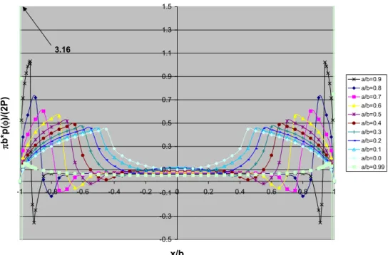
0 0.5 1 1.5 2 2.5 -1 -0.8 -0.6 -0.4 -0.2 0 0.2 0.4 0.6 0.8 1 x/b π b*p( φ )/(2P) a/b=0.9 a/b=0.8 a/b=0.7 a/b=0.6 a/b=0.5 a/b=0.4 a/b=0.3 a/b=0.2 a/b=0.1 a/b=0.0 a/b=0.99 6.34

Figure 1-11: The normalized pressure distribution for a flat punch of length 2a with rounded corners resulting in contact length 2b. Various values a/b are shown.

1.3.4 Other geometries

Consider a punch that has a flat region of length 2a with a rounded corner of radius D/2. Under a normal load, the contact length becomes 2b. The contact pressure of such a punch in contact with a semi-infinite substrate was given by Ciavarella [30]

πb 2Pp (φ) = 1 π − 2φo− sin (2φo) [(π − 2φo) cos φ + ln (G(φ))] ; |x| ≤ b (1.41) G(φ) = ¯ ¯ ¯ ¯ sin (φ + φ_o) sin(φ − φo) ¯ ¯ ¯ ¯ sin φ × ¯ ¯ ¯ ¯tan φ + φ_o 2 tan φ − φo 2 ¯ ¯ ¯ ¯ sin φo (1.42) where

(33)

The pressure distributions for values of a/b are shown in Figure 1-11. The relationship between b and P is given by

P D a2_E∗ =

π − 2φo

2 sin2φ_o − cot φo (1.44)

In conditions of partial slip, a stick zone cannot be sustained within the flat region of the punch [26]. In other words, the magnitude of c must be greater than that of a. The relationship between Q and c becomes[31]

Q f P = 1 − ³c b ´2 _{π − 2θ}_o_{− sin (2θ}_o₎ π − 2φo− sin (2φo) (1.45) where

sin θo = a/c; sin φo= a/b (1.46)

The shear tractions are defined as

q(x) = f p(x); _{b ≤ |x| ≤ c} (1.47)

q(x) = f [p(x) − q∗(x)] ; a ≤ |x| ≤ c (1.48)

where q∗(x) is the same as p(x) above replacing φ and φ_owith θ and θo. The normalized shear tractions for various a/b are shown in Figure 1-12.

The contact pressure and the shear tractions become singular as b equals a, while they approach the Cattaneo-Mindlin solution as a goes to zero. Figure 1-13 shows compares a/b=0.9 to the Cattaneo-Mindlin solution at a/b=0.0.

In engineering practice, a plethora of contact geometries exist. For the most complex geometries and loadings, there is often no choice but to use numerical models such as finite element analysis to obtain contact stresses and relative displacements. Finite element meshes must be very dense in the region of contact because of the steep strain and displacement gradients. Optimal meshes, balancing computational eﬃciency and solution accuracy, must be carefully designed. If sharp corners are present, one may choose to use crack-tip finite elements

(34)

-0.5 -0.3 -0.1 0.1 0.3 0.5 0.7 0.9 1.1 1.3 1.5 -1 -0.8 -0.6 -0.4 -0.2 0 0.2 0.4 0.6 0.8 1 x/b π b*p( φ )/(2P) a/b=0.9 a/b=0.8 a/b=0.7 a/b=0.6 a/b=0.5 a/b=0.4 a/b=0.3 a/b=0.2 a/b=0.1 a/b=0.0 a/b=0.99 3.16

(35)

-0.5 0 0.5 1 1.5 2 2.5 3 -1 -0.8 -0.6 -0.4 -0.2 0 0.2 0.4 0.6 0.8 1 x/b π b*p( φ

)/(2P) a/b=0.9, sheara/b=0.9,normal a/b=0.0, shear a/b=0.0, normal

Figure 1-13: The pressure and shear tractions are shown for two extremes of the flat punch with rounded corners: a/b=0.9 and a/b=0.0 for Q/fP =0.8.

(36)

(37)

Chapter 2

Overview of highly controlled

fretting fatigue experiments

2.1 Introduction

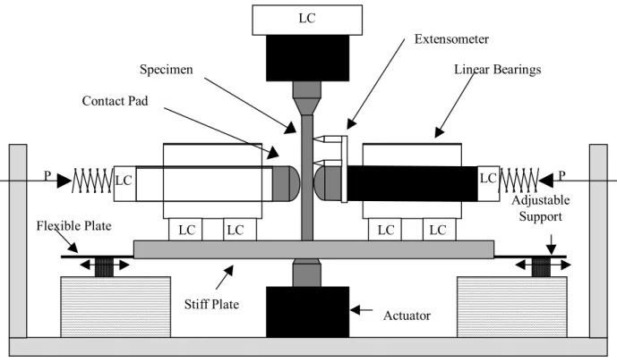
As researchers determined critical variables to fretting fatigue damage, fretting fatigue fixtures had to be designed to control and instrument these variables. These variables would include the normal load, P ; the tangential load, Q; the bulk load, F ; and the displacement. A fretting fatigue fixture developed at MIT enables the researcher to control and measure every major fretting fatigue variable, see Figure 2-1.

2.2 Description of the apparatus

Loads are controlled in several ways. A servo-hydraulic testing machine provides the bulk load to the specimen. The normal load is applied through the compression of springs against a shaft held by linear bearings. Interchangeable contact pads are fixed to the end of the shaft opposite from the springs. The shaft is held in place by a linear bearing. The bearing and a fluid lubricant reduce friction, allow for maximum transfer of force from the springs to the contact pad. A load cell between the spring and the shaft measures the normal force, P . A frictional force, Q, that is tangent to the contact interface develops with application of the bulk load, F . Load cells underneath the mounts containing the linear bearings measure Q.

(38)

An extensometer was developed to measure global displacement. The extensometer is attached behind one of the fretting pads. It has two sharp prongs. One is aﬃxed to the shaft directly behind the pad. The other is glued to the specimen surface at nearly 25 mm away from the center of contact. A schematic of the fixture, the extensometer and the load cells is shown in Figure 2-2.

The signals from each load cells are sent to a data card on a nearly PC. The voltages are converted into loads or displacements by a LabView program. The LabView program displays the inputs from the load cells in real time and records data at predetermined intervals.

2.2.1 The relationship between the tangential load and the bulk load

The bearing mount rests upon a stiff plate supported by flexible sheets at each end. Moveable blocks attach the sheet to the rigid supporting structure affixed to the servo-hydraulic machine. The location of the blocks determine the amount of compliance in the tangential load train, Cq. The compliance of the bulk load train, Cf,can be changed by inserting one end of the specimen into either a stiff or compliant fixture. The tangential load is related to the application of the bulk load by the following relationship

Q = − µ Cf Cq ¶ F (2.1)

This relationship serves as a guide for experiment setup (e.g. one must apply a specific F to produce a Q) and must be determined experimentally. It should be noted that the tangential and bulk loads are in-phase.

2.3 Description of experiments

The specimens are bar specimens with a square cross sectional area. The pads are spherical and screw into the rods. Tests can be run up to a pre-determined number of cycles or to failure. Upon failure, tension on the specimen would result in a rapid increase in displacement of the actuator. If the pre-programmed displacement limits are exceeded, the test will stop. Small variations in the loading waveform require that the displacement limits be set on the order of 0.5 mm. As a result, the contact region is often scratched and damaged upon failure,

(39)

Figure 2-1: A photograph of the MIT fretting fatigue fixture. The extensometer can be clearly seen to the left of the specimen. The width of the bar specimen is 4.74 mm.

Specimen Contact Pad P P Actuator LC LC LC LC LC LC Linear Bearings Stiff Plate Flexible Plate Extensometer Adjustable Support LC

Figure 2-2: A schematic of the MIT fretting fatigue fixture showing the location of load cells, applied loads and supports.

(40)

E (GPa) ν σy (MPa) σTS (MPa) σTF (MPa) Tens el. (%) RA (%) SR (s−1)

116 0.3 930 965 1310 19 45 _8×10−4

Table 2.1: A list of some of the mechanical properties of the Ti-6Al-4V alloy. TS=tensile strength. TF=true fracture stress. RA=reduction in area at fracture. SR=strain rate

so information is limited. Interrupting tests can determine the dimensions of a fretting scar and location of cracks (if they have initiated) compared to the contact radius and slip region.

2.3.1 Material

Ti-6Al-4V was the material selected for the controlled fretting fatigue experiments as well as the dovetail fretting fatigue experiments described in the next chapter [37, 56]. Most of the tests were performed on two heat treatments: mill annealed (MA) and solution treated over-aged (STOA). The MA and STOA materials had very similar fretting fatigue behavior and mechanical properties. Some of the mechanical properties of the STOA material are shown in Table 2.1 [57]. Fatigue behavior at various R can be found in [58].

2.3.2 Experimental matrix

A matrix of experiments was established to consider the effect of changing individual loads while maintaining all others constant. The load ratio (defined as R = Lmin/Lmax) was -1 in all of the fretting fatigue experiments performed with this apparatus. The first category of experiments involved changing the maximum bulk load while keeping contact loads constant. This is very similar to fretting fatigue tests found in the early literature and demonstrate the effect of fretting fatigue on the fatigue strength. The second set of experiments involved changing the normal load for each test while keeping Q constant at 17 N and the maximum bulk load constant at 300 MPa. By increasing the normal, the contact area and the contact pressure also increase. Finally, the tangential load was modified in each test as the P constant at 50 N and the maximum bulk load constant at 300 MPa. As Q is increased, the size of the slip region increases until it covers the entire contact surface and global sliding occurs. Below a certain Q, the impact of fretting fatigue on fatigue life is minimized, but Q greater than f P results in sliding. For each category of tests, one other variable was considered: changing the pad radius from 12.7 mm to 25.4 mm. Table 2.2 shows the effect of changing pad radius on

(41)

Pad radius (mm) Load (N) a (µm) po (MPa) w (N/m) amax (µm)

12.7 50 194 637 1 237

25.4 50 244 401 1 298

Table 2.2: Contact radii and pressures for Ti-6Al-4V pads pressed into a flat surface at 50 N.

200 250 300 350 400 450 500 550

1.E+04 1.E+05 1.E+06 1.E+07

Number of cycles to failure

Maximum bulk stress (MPa), R=-1

R=25.4 mm, Q=30 N, N=50 N R=12.7 mm, Q=30 N, N=50 N R=25.4 mm, Q=15 N, N=50 N R=12.7 mm, Q=15 N, N=50 N Plain Fatigue, Bellows et al.

Arrow denotes runout

Figure 2-3: The first series of experiments varied the maximum bulk stress applied in each test for several contact conditions. The results are compared with plain fatigue data from Bellows et al. [58].

contact radius and pressure.

Experimental results are plotted in Figures 2-3 to 2-5. The following statements could be made:

1.) Compared with plain fatigue, fretting fatigue reduces the maximum bulk stress required for failure at a given life. This is known as the ”knockdown” eﬀect [59] and a knockdown factor can be computed:

(42)

0 0.1 0.2 0.3 0.4 0.5 0.6 0.7 0.8

1.E+05 1.E+06 1.E+07

Q/P

Pad radius of 12.7 mm Pad radius of 25.4 mm

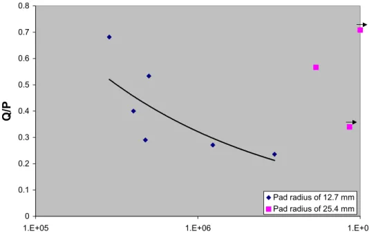
Figure 2-4: Keeping Q fixed at 17 N, P is varied. The maximum bulk stress is 300 MPa. Notice the eﬀect of increasing the pad radius from 12.7 mm to 25.4 mm.

(43)

0 0.1 0.2 0.3 0.4 0.5 0.6 0.7

1.E+05 1.E+06 1.E+07

Q/P

Pad radius of 12.7 mm Pad radius of 25.4 mm

Figure 2-5: The tangential load is varied for each test while P is held at 50 N. Again, a decrease in the pad radius results in a decrease in the fretting fatigue life at a given Q/P .

(44)

kf = σf,f f σf,pf

(2.3)

The controlled fretting fatigue experiments shown in Figure 2-3 demonstrates that kf is reduced when Q is increased and P is held constant for a given pad radius. kf is also reduced when the pad radius is reduced and contact loads remain constant. It should be noted that fretting fatigue life is also reduced when the maximum bulk stress is increased and all other conditions are held constant.

2.) If the normal load is held constant, the fretting fatigue life decreases as Q is increased. The fretting fatigue life will decrease even further if the pad radius is reduced.

3.) If the tangential load is held constant, increasing P will increase fretting fatigue life. However, reduction in the pad radius will still decrease fretting fatigue life.

Scar description and crack initiation location

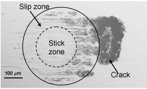
Wear is produced as a result of slip in the region between the stick zone and the edge of contact. Oxides are produced as fresh material is exposed. For a Ti-6Al-4V on Ti-6Al-4V contact, this oxide is dark and produces a ring about the stick zone called the fretting scar, shown in Figure 2-6.

When cracks did initiate, they did so only at the region near the edge of contact closest to the actuator (x = −a, y = 0). This is because the bulk stress is tensile and the contact stresses are tensile at the same time, see Figure 2-7. “Near” the edge of contact is defined as at the edge of contact, in the slip zone, or just outside of the edge of contact. The crack in 2-6 is just outside of the contact zone.

Further analysis of these results will be presented in Chapter 5 when a fracture mechanics based life prediction method is applied.

(45)

Figure 2-6: A fretting fatigue scar for a specimen after 10,000,000 cycles (P =24 N, Q=17 N, pad radius of 25.4 mm and max bulk stress of 300 MPa). A crack developed but did not propagate to failure.

Figure 2-7: In the sphere-on-flat experiments, cracks would initiate only on the side closest to the actuator.

(46)

Chapter 3

Development of a dovetail fretting

fixture

A typical fretting fatigue apparatus applies a constant normal load through springs or bolts. Fretting is possible when both the normal and tangential loads are cyclic. There are two methods to perform this in an experimental fixture. The first is to use the typical fretting fatigue fixture but add an actuator in the contact load train to apply the cyclic normal load. The second is to develop a dovetail fixture. Both types of fretting fixtures have been developed.

Ruiz developed a dovetail fretting fatigue fixture and validated his fretting fatigue parameter with experiments [27, 28, 60]. Two or six dovetail shaped specimens are held in dovetail slots on opposite sides of a sheet. One actuator pulls on the dovetails while another places the sheet in tension. This simulates the inertial loading in a gas turbine engine. Recently, the Oxford group added the capability of a bending moment on the dovetail specimen to simulate blade bending as a result of airflow. The contact between the blade and the sheet is fully conformal on the Ruiz fixture unlike basic contact geometries often found in the literature. The advantage of the Ruiz fixture is that it is very similar to the real blade-disk dovetail joints in gas turbine engines.

To bridge the gap between real contact geometries and more fundamental geometries, a new dovetail fixture was developed at the U. S. Air Force Research Laboratory (AFRL), see Figures 3-1 and 3-2. Rather than use a fully conformal contact geometry as in the Ruiz fixture, the

(47)

Figure 3-1: A photograph of the dovetail fixture and specimen.

AFRL fixture holds removable contact pads that can be made of any geometry or material. The fixture itself is made of 4140 steel with a Young’s modulus of 205 GPa and Poisson’s ratio of 0.27. It is held by a bolt at the top. The specimens and pads are placed into the fixture from the side. The specimen is loaded in tension only since compression would cause the specimen to impact the dovetail slot. The specimen is gripped by friction either by collet grips or friction grips and loaded by a hydraulic actuator.

Early finite element modeling showed a region of compressive strain of large magnitude on the face of the fixture located across from the high stress concentration of the dovetail slot, see Figure 3-2. A strain gauge was placed at this location to validate finite element modeling. This is discussed further below.

3.1 Experimental results

All experiments used Ti-6Al-4V specimens and pads. Three contact geometries were chosen. The first is a 1.016 mm flat pad with an 11◦ taper and a blend radius of approximately 1 mm. Next is a 6.35 mm flat pad with rounded corners of radius 3.175 mm. Finally, a cylindrical pad was chosen to provide a Hertzian pressure distribution. It has a radius of 50.8mm. These geometries will be referred to as the “short flat”, “long flat” and “cylindrical” pads.

(48)

Figure 3-2: A schematic of the dovetail fretting fatigue fixture.

The specimens were tested with a step testing methodology. This method was first derived to develop rapidly a high cycle fatigue (107 cycles) Haigh diagram experimentally [61]. It was later validated for fretting fatigue testing [62]. The method is as follows. A load is applied to the specimen at a given load ratio but at a maximum load below that which is expected to cause failure. If failure does not occur after a specified number of cycles, No, the maximum load is increased by a predetermined step increment, but the same load ratio is maintained. The load is stepped up until failure occurs at a given step, n. The load at failure, Ff, and the number of cycles to failure at step n, Nf,n is recorded. Since a predetermined step increment was used at each step, the load at the step prior to failure, Fpr, is also known. The load required to cause failure at No cycles, Fi, can now be determined using the following equation:

Fi= Fpr+ Nf,n

No

(Ff − Fpr) (3.1)

In all of the tests that were designed to lead to failure, No was 106 cycles. A summary of all of the dovetail fretting fatigue tests is given in Table 3.1. The first series of tests were performed at a frequency of 30 Hz and load ratio of 0.1. All three of the pad geometries were used. It was demonstrated that the long flat pad could sustain the largest maximum load, an

(49)

Figure 3-3: A large crack developed near the maximum edge of contact in Specimen # T2.

average of 20.1 kN, to failure after 106 cycles. This geometry was followed by the cylindrical pad with an average maximum load of 19 kN while the short flat geometry could only sustain a mean maximum load of 18.3 kN. When the load ratio was increased to 0.5, the short flat pad sustained a maximum load of 21 kN.

The dominant crack (i.e. the one that will propagate to failure) is located near the maximum edge of contact on the side of the specimen closest to the actuator. This is shown in the SEM image of the fretting scar in Figure 3-3. A section of that scar reveals that cracks initiated in the slip regions near both sides of the maximum contact length, see Figure 3-4. The dominant crack will always be near the edge closest to the actuator since the maximum bulk stress and the maximum contact stresses occur during the same portion of the loading cycle.

Using the mean maximum loads above, strain gauge measurements were made during the fretting fatigue experiments. Measurements were taken as early as 3 cycles after the test start and as late as 100,000 cycles. The test frequency was reduced since the data acquisition software could not take data at frequencies faster than 10 Hz.

A CCD camera was focused on the near contact region. Using a software algorithm devel-oped at AFRL, displacements near the region of contact were measured [63]. During filming, the test frequency was dropped to 0.001 Hz. To film at higher frequencies would require a synchronized strobe light. The CCD images recorded gross relative contact displacements. For the short flat geometry with a maximum load of 18.3 kN at R=0.1, the global relative displacement during the second cycle of loading was 18 microns. In the case of the cylindrical

(50)

Figure 3-4: A section taken from the scar in the previous figure shows that cracks have developed in the slip regions near both edges of maximum contact length. The largest crack is the same crack visible in the previous figure.

with a maximum load of 19.0 kN at R=0.1, the global displacement during the second cycle of loading was 23 microns.

3.1.1 Fretting fatigue scar measurement

Several of the fretting fatigue scars were measured from micrographs taken after fretting fatigue tests. The measurements of the contact length, 2a or 2b, and the length of the stick zone, 2c, (recall definitions of a, b, and c from Chapter 1) are listed in Table 3.2. The presence of stick zones underneath the flat portion of the contact is in direct disagreement with theory from [26]. There are two posssible reasons for the presence of the stick zones. The first is that corners may become rounded as a result of wear during the fretting fatigue test. The second is that the flat region of the contact pad may not truly be flat but cylindrical with a very large radius of curvature as a result of machining and tumbling. ‘

(51)

Specimen # Pad R f (Hz) Ff Fpr Fi n Nf,n Result

T2 short flat 0.1 30 18 16 16.7 5 351,094 failure

01-590 short flat 0.1 30 19 18.5 18.6 3 239,291 failure

01-595 short flat 0.1 30 18.5 18 18.5 2 926,097 failure

01-593 short flat 0.1 30 18 n/a 18 0 892,301 failure

01-479 short flat 0.1 30 18.3 n/a 18.3 0 1,400,000 failure

01-598 long flat 0.1 30 20.5 20 20.1 6 213,988 failure

01-599 long flat 0.1 30 20 19.5 19.5 3 14,575 failure

01-601 long flat 0.1 30 21 20.5 20.6 5 227,441 failure

01-478 cylindrical 0.1 30 20 18 19.5 3 770,828 failure

01-596 cylindrical 0.1 30 19.5 19 19.4 4 888,192 failure

01-597 cylindrical 0.1 30 19 18.5 18.7 2 305,585 failure

01-594 cylindrical 0.1 30 19 18.5 18.8 2 557,008 failure

01-465 short flat 0.1 10 18.3 n/a n/a 0 33,324 interrupted, sg

01-466 long flat 0.1 10 20.1 n/a n/a 0 100,000 interrupted, sg

01-467 cylindrical 0.1 10 19 n/a n/a 0 100,000 interrupted, sg

01-468 short flat 0.1 10 20.1 n/a n/a 0 100,000 interrupted, sg

01-473 cylindrical 0.1 30/0.001 19 n/a n/a 0 500 interrupted, vm

01-472 short flat 0.1 30/0.001 18.3 n/a n/a 0 500 interrupted, vm

01-477 short flat 0.5 30/0.001 18.3 n/a n/a 0 500 interrupted, vm

Table 3.1: Experimental results from dovetail fretting tests. Loads in kN; sg=strain gauge; vm=video strain mapping.

Specimen Geometry Flat length (mm) 2a or 2b (mm) 2c (mm)

T2 short flat 1.016 1.21 0.73

01-590 short flat 1.016 1.22 0.69

01-479 short flat 1.016 1.36 0.96

01-594 cylindrical 0 2.36 1.58

01-598 long flat 6.35 4.64 2.32

(52)

Head E (GPa) v

Ti-6Al-4V 116 0.3

4140 Steel 125 0.3

Table 3.3: Elastic properties of materials used in finite element model of the dovetail.

3.2 Numerical simulation of fretting fatigue in a dovetail fixture

A 2-D global finite element model of the dovetail fretting apparatus was developed. Using symmetry boundary conditions at the fixture centerline, only the right side of the fixture is modeled. The mesh of the fixture itself is coarse compared to the mesh in the contact region. Convergence plots were used to determine the necessary element size to obtain accuracy of the vertical elastic strain in the region of the strain gauge.

The contact pads were integrated into the fixture (rather than placed in slots) so the model would be well supported. However, the contact pads were partitioned apart from the remainder of the fixture, so that the mechanical properties of the Ti-6Al-4V could be applied to the pads while the mechanical properties of 4140 steel were applied to the fixture, see Table 3.3.

The fixture was rigidly supported at the bolt hole and was found to produce the equivalent strains as placing a fixed, frictionless rigid cylinder into the bolt hole. A pressure was applied to the base of the specimen equivalent to the applied load divided by half the specimen cross-sectional area (the factor of one-half due to symmetry).

4 node plane strain elements (ABAQUS CPE4R) were chosen. The deformation was taken to be fully elastic. The global mesh is shown in Figure 3-5. Near the contact, the length of an element side was approximately 8 microns. For the loads in the cylinder dovetail experiment, there are nearly 270 elements in the contact region. For the short flat experiment, there are nearly 130 elements in the contact region as shown in Figure 3-6. Smaller elements would have been computationally too costly for this scale of model. The surface of the pad and the opposing specimen surface were chosen to be a contact pair.

A Langrangian multiplier method was selected to enforce stick-slip constraints at the surface. The Langrangian method prevents relative motion between two surfaces until the shear traction exceeds a critical value [64]. This adds more degrees of freedom to the model; therefore, it is more computationally expensive than say a penalty friction method which allows sticking nodes

(53)

Figure 3-5: The global mesh for the dovetail finite element model. Notice that the mesh in both the specimen and the fixture becomes refined closer to the interface.

Figure 3-6: In the case of the short flat contact geometry, nearly 130 elements are located near the contact region.

(54)

Figure 3-7: The calculated hystersis loop over two cycles of loading for several values of the coeﬃcient of friction.

to slip to increase eﬃciency. However, partial-slip conditions would not be accurately modeled with a penalty method, so the cost must be accepted. A coeﬃcient of friction of 0.5 was chosen for all models except that of the coated dovetail which had f=0.2. More will be said on the coated dovetail in the chapter on palliatives.

To obtain a stable hysteresis loop, two cycles of loading are performed. Each half cycle was broken into 15 steps. The steps were the minimum load, 5% of the cycle’s half-period, 10%, 20%, 30%, 40%, 50%, 60%, 70%, 80%, 90%, 95%, 97.5% and maximum load. The reduction of step size near maximum load was necessary for the model to converge.

The evolution of friction during the first two cycles was examined by plotting the calculated strain versus the applied bulk load to the dovetail specimen. As shown in Figure 3-7, the shape of the curve is strongly influenced by the coefficient of friction. The hysteresis loop becomes closed as the coefficient of friction increases. The response in the model is not as stiff as the actual response measured by the strain gauges, see Figure 3-8. This may be the result of the two dimensional nature of the model or an error in the material properties.

(55)

Figure 3-8: The strain versus load response measured at the strain gauge compared to the calculated response from the model.

3.2.1 Obtaining point loads from the finite element model

As presented earlier, determining contact point loads is impossible without outside information (numerical modeling or devices such as the strain gauge) since the loads are statically inde-terminate. An infinite number of magnitudes of P and Q could be found for a given F. One approach numerically, would be to use a cylindrical contact geometry for the desired F (even if the actual contact geometry is not cylindrical). The cylindrical contact will produce a parabolic pressure distribution with known relationships for a and P. Since the pressure goes to zero at the edge of contact, one can determine a, then P can be found.

An understanding of the applied forces will help. Consider the dovetail shown in Figure 3-9. Three points are shown. A force F is applied in the x2direction to the bottom cylindrical portion of the specimen at point A. The two points along the flanks of dovetail represent the centroid of the contact. These are named points L and R for left and right. The following assumptions are made. First, that the contact problem can be modeled using static equilibrium (i.e. PFi = 0,PMi = 0). There are no body forces in this model. Second, the contact loads

Contact fatigue : life prediction and palliatives

Contact Fatigue: Life Prediction and Palliatives

by

Brett P. Conner

B.S., University of Missouri-Columbia (1998)

S.M., Massachusetts Institute of Technology (2000)

Submitted to the Department of Materials Science and Engineering

in partial fulfillment of the requirements for the degree of

Doctor of Philosophy

at the

MASSACHUSETTS INSTITUTE OF TECHNOLOGY

September 2002

c

° 2002 Massachusetts Institute of Technology. All rights reserved.

The author hereby grants to Massachusetts Institute of Technology permission to

reproduce and

to distribute copies of this thesis document in whole or in part.

Signature of Author . . . .

Department of Materials Science and Engineering

20 August 2002

Certified by . . . .

Subra Suresh

R. P. Simmons Professor and Head, Department of Materials Science and Engineering

Thesis Supervisor

Accepted by. . . .

Harry L. Tuller

Contact Fatigue: Life Prediction and Palliatives

by

Brett P. Conner

Abstract

Contents

List of Figures

List of Tables

Chapter 1

Introduction

1.1

Background

1.1.1

Historical perspectives on fretting fatigue

1.1.2

Recent developments

1.2

Contact fatigue in aerospace materials

1.3

Contact Mechanics

1.3.1

Normal Contact

1.3.2

Contact in the presence of friction

1.3.3

Contact in the presence of adhesive forces

1.3.4

Other geometries

Chapter 2

Overview of highly controlled

fretting fatigue experiments

2.1

Introduction

2.2

Description of the apparatus

2.2.1

The relationship between the tangential load and the bulk load

2.3

Description of experiments

2.3.1

Material

2.3.2

Experimental matrix

Chapter 3

Development of a dovetail fretting

fixture

3.1

Experimental results

3.1.1

Fretting fatigue scar measurement

3.2

Numerical simulation of fretting fatigue in a dovetail fixture

3.2.1

Obtaining point loads from the finite element model