HAL Id: tel-01324110
https://hal.archives-ouvertes.fr/tel-01324110
Submitted on 31 May 2016
HAL is a multi-disciplinary open access
archive for the deposit and dissemination of sci-entific research documents, whether they are pub-lished or not. The documents may come from teaching and research institutions in France or abroad, or from public or private research centers.
L’archive ouverte pluridisciplinaire HAL, est destinée au dépôt et à la diffusion de documents scientifiques de niveau recherche, publiés ou non, émanant des établissements d’enseignement et de recherche français ou étrangers, des laboratoires publics ou privés.
Subsurface stress inversion modeling using linear
elasticity : sensivity analysis and applications
Mostfa Lejri
To cite this version:
Mostfa Lejri. Subsurface stress inversion modeling using linear elasticity : sensivity analysis and applications. Geophysics [physics.geo-ph]. Université de Montpellier, 2015. English. �tel-01324110�
Délivré par l’Université de Montpellier
Préparée au sein de l’école doctorale SIBAGHE
Et de l’équipe de recherche BASSINS
Spécialité : GEOSCIENCES
Présentée par LEJRI Mostfa (Mustapha)
Soutenance prévue le 02 Juillet 2015 devant le jury composé de :
Dr. Roger Soliva, Université Montpellier Directeur de thèse
Dr. Laurent Maerten, Schlumberger Co-Directeur
Dr. Frantz Maerten, Schlumberger Co-Directeur
Pr. Olivier Lacombe, Université Paris VI Rapporteur
Pr. Jean Pierre Gratier, Université de Grenoble Rapporteur
Pr. Rodolphe Cattin, Université Montpellier Examinateur
Dr. Bertrand Gauthier, Total Examinateur
Dr. Bernard Célérier, Université Montpellier Examinateur
SUBSURFACE STRESS INVERSION
MODELING USING LINEAR
ELASTICITY: SENSITIVITY ANALYSIS
AND APPLICATIONS
Avant-propos
Cette thèse a été co-financée par une bourse CIFRE (ANRT) et l’entreprise Schlumberger sous l’égide du
laboratoire de géosciences de l’université de Montpellier. Elle s’est déroulée en majeure partie au sein des
locaux de Schlumberger MpTC à Montpellier.
Le présent manuscrit est constitué de quatre articles scientifiques. Le premier est publié dans la revue
Tectonophysics, le second est en préparation pour la revue Tectonophysics. Les troisième et quatrième
articles sont en préparation pour Structural geology et le journal de l’AAPG. Par conséquent, le format des
chapitres est présenté en anglais sous la forme d’articles scientifiques.
Remerciements
Mon experience pendant cette thèse CIFRE au sein de Schlumberger a été intellectuellement stimulante
et enrichissante au dela des espérances. Cette thèse n’aurait pas été possible sans l’implication et la
contribution intellectuelle de plusieurs personnes que ce soit au sein de Schlumberger, de l’université de
Montpellier ou dans mon entourage.
Je tiens d’abord à remercier très chaleureusement mes directeurs de thèse Laurent Maerten qui m’a
transmis son savoir sur la géologie structurale et m’a appris, à travers son oeuil expert et une pédagogie
exceptionnelle, à raisonner et écrire en tant que scientifique, et Frantz Maerten qui, par son génie et avec
beaucoup d’humour, m’a donné goût à la programmation et à la mécanique des failles. Ils ont su m’épauler
durant ces années, et m’ont insufflé leur enthousiasme, leur vision et leur passion pour la géologie, la
modélisation numérique et la géomécanique. Je remercie au même titre Roger Soliva qui m’a transmis sa
passion de la géologie structurale, il a été pour moi un exemple de rigeur dans le travail et m’a guidé tout au
long de cette aventure. Plus que des mentors vous avez été de véritables amis.
Je voudrais spécialement remercier Emmanuel Malvesin, qui tout au long de ces années a été un ami,
d’un conseil avisé, et un motivateur incontournable, “la fine fleur…” ainsi que Jean Pierre Joonnekindt qui a
été un grand soutient, et Nader Salman, un co-leader exceptionnel.
Je remercie biensur Alex Wilson, qui a suivi tout mon parcours et oeuvré pour mon integration au sein
de Schlumberger. Un grand merci aux collègues à Schlumberger MpTC, et plus particulièrement, Stéphane
Bonassies et Christelle Guilermou qui ont oeuvré afin que ma these se déroule dans les meilleures conditions
possibles. J’en profite également pour remercier toutes les personnes qui m’ont soutenu de près ou de loin
(dans le désordre): Claire Maerten, Aloïse Chabert pour sa bonne humeur constante, Joan Mouba , Pauline
à la dernière minute, Berangère Guerry et Sarah Macaud pour leurs encouragements, Martin Neumeyer
pour sa passion de géologie et les discussions enrichissantes, Naouel Arbi pour son aide et ses
encouragements depuis mon arrive à Schlumberger, Marie LeFranc, Saad Kisra, Fabrice, Paxi, Phil Resor,
Mathieu, Terje, Jimmy, Michael, David, Illike, Gayana, Thibault Cavailhes, Marine Dalmasso… Bertrand
Gauthier qui a été d’un grand conseil et pour sa confiance en moi lors du workshop à Total, Olivier Lacombe
pour m’avoir permis d’approfondir mes connaissances et m’avoir acceuilli à L’EGU, Bernard Célérier pour ses
conseils et corrections post-soutenance, et Romain Plateaux pour son enthousiasme et sa lecture
constructive du manuscrit… vous avez tous été la et je garde de vous un souvenir impérissable.
Merci à Ali Mehez, Fares Bouhlila et Adlène Mallem et qui ont été des frères pour moi durant ces années
d’études. Un immense merci à Axelle Riou qui a été présente pour moi à chaque instant. Merci également à
Sandrine Riou et Michel Portant, votre presence a été pour moi très importante. Et bien sûr, un grand merci
à Marie-France Roch pour son assistance depuis le Master et aux equipes du laboratoire géosciences et
particulièrement Michel Serannes pour son suivi et son intransigence. Enfin je remercie les membres de ma
famille qui m’ont encouragé depuis le plus jeune age dans ma passion pour les sciences et en particulier mon
père Mohamed Lamine Lejri et ma mère Nejia Lejri à qui je dédie ce travail.
Lejri Mostfa, Juillet 2015
« If i have seen further than others, it is by standing upon the shoulders of giants » Isaac Newton
Table of Contents
Extended abstract 1
General introduction 5
1.Essence of the thesis 5
2.How are the fractures modeled in the Oil & gas industry? 6
2.1. Existing techniques 6
2.2. Techniques based on geomechanics 7
3.Faults and Fractures 9
3.1. Faults, fault systems and stress field 10
3.2. Fault genesis and tectonic regimes 12
3.3. Fault reactivation 14
3.4. Fault sliding friction 16
3.5. Fractures classification and stress field 18
3.6. Fractures related to faulting 19
3.6.1. Fracture genetically associated to faulting 19
3.6.2. Fracture not genetically associated to faulting 20
4.How to recover paleostresses? 22
4.1. Paleostress estimation using Wallace & Bott type methods 23
The Wallace (1951) and Bott (1959) hypothesis 23
4.1.1. The stress ratio (R) 24
4.1.2. The forward problem 25
4.1.3. Stress inversion problem 26
4.1.4. Stress inversion using slip data 28
4.1.5. Stress inversion using focal mechanisms 31
4.1.6. Stress inversion using calcite twins 34
4.2. Polyphase tectonic events 36
4.2.1. The polyphase data problem 36
4.2.2. Existing methods to separate tectonic phases 37
4.3. Methods based on geomechanics 40
4.3.1. Least squares formulation (Kaven et al., 2011) 40
4.3.2. iBem3D (Maerten et al., 2014) 40
5.Methods (after Maerten et al., 2014) 41
5.1. iBem3D - iterative boundary elements method 42
5.1.1. Far field stress/strain 44
5.1.2. Research applications 44
5.1.3. Industry and engineering applications 50
5.1.4. Latest enhancements 55
5.2. BEM-based stress inversion method 57
5.2.1. Principle of superposition 59
5.2.2. Real time computation 60
5.2.3. Method of Resolution 61
5.2.5. Tectonic stress domain 64
6.Problematics of the thesis: 65
References 67
CHAPTER I: Paleostress inversion: A multi-parametric geomechanical evaluation of the Wallace-Bott
assumptions 95 Abstract 95 1.Introduction 96 2.Method 99 2.1. Numerical tool 99 2.2. Fault geometry 100 2.3. Tectonic stress 103 2.3. Fault friction 104
2.4. Fault fluid pressure 105
2.5. Traction free surface of the Earth 105
2.6. Poisson’s ratio 106
2.7. Non-tested parameters 107
2.8. Mean misfit angle calculation and domain representation 107
3.Results 111
3.1. Effect of fault geometry 111
3.1.1. Single planar fault 111
3.1.2. Intersecting faults 112
3.1.3. Sinusoidal faults 115
3.2. Effect of the traction free surface of the Earth 116
3.3. Effect of Poisson’s ratio 117
3.4. Effect of fault friction 118
3.5. Effect of fault fluid pressure 120
4.Discussion 121
4.1. Fault geometry 121
4.2. Traction free surface 125
4.3. Poisson's ratio 125
4.4. Fault friction 126
4.5. Fault fluid pressure 126
4.6. Complementary study 126
5.Conclusions 129
Acknowledgements 131
References 132
CHAPTER II: Accuracy evaluation of both Wallace-Bott and BEM-based paleostress inversion methods 143
Abstract 143
1.Introduction 144
2.Method 147
2.1. Stress inversion methods 147
2.3. Tectonic stress 150
2.4. Sliding friction 151
2.5. Data sampling 152
2.6. Analysis procedure 152
3.Analyses 155
3.1. Relationship between 𝝎 and 𝜟 155
3.2. Sliding friction effect 158
3.3. Sampling effect 161
4.Chimney Rock case study 162
4.1. Geologic setting and previous models 163
4.2. Fault model configuration 167
4.3. Stress inversions and sampling methodology 168
4.4. Stress inversions accuracy prediction domain 172
5.Discussion 173
5.1. Relationship between 𝝎 and 𝜟 173
5.2. Sliding friction 175
5.3. Data sampling 177
5.4. Chimney rock 177
Stress inversion and sampling 177
Chimney rock fault array evolution 179
Predition domain 179 6.Conclusions 180 Acknowledgements: 184 Tables 185 Annex 187 References 190
CHAPTER III: Geomechanical paleostress inversion using fracture data: Application to modeling natural
fractures in reservoirs 199 Abstract 199 1.Introduction 200 2.Method 204 2.1. Numerical tool 205 2.2. Fault Paleo-Geometry 206
2.3. Paleo tectonic stresses 207
2.3.1. Parameter Space 207
2.3.2. Computation Time 209
2.3.3. Fracture data and cost functions 210
2.3.4. Tectonic stress domain 212
2.3.5. Under-constrained model 213
3.Nash Point outcrop case study 216
3.2. Paleostress inversion 219
3.2.1. Model configuration 220
3.2.2. Model results 221
3.2.3. Sensitivity to fracture data location 223
3.3. Joint trajectory convergence investigation 225
3.3.1. Contact point model 225
3.3.2. Fluid pressure model 227
4.Les Matelles outcrop case study 229
4.1. Geological Setting 230
4.2. Paleostress inversion 232
4.2.1. Model configuration 232
4.2.2. Model results 233
4.2.3. Sensitivity to 3D fault model geometry 237
4.3. Influence of fault friction 238
5.Oseberg Sør field case study 240
5.1. Geological Setting 241
5.2. Paleostress inversion 242
5.2.1. Model configuration 242
5.2.2. Model Results 244
6.Discussion and conclusions 245
6.1. The method 245
6.2. The Nash Point example 247
6.3. The Matelles example 249
6.4. The Oseberg Sør example 250
6.5. Further applications 251
Acknowledgments 252
References 253
Annex 1: 260
Annex 2: 260
CHAPTER IV: Polyphasic geomechanical stress inversion using undefined fractures mechanical type 265
Abstract 265
1.Introduction 266
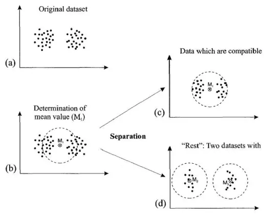
The determination of multiple tectonic events 267
The oil industry problem: multiple phases and unknown fracture types. 269
Our approach 270
2.Methods and synthetic models validation 271
Numerical methods 271
2.1.1. BEM 271
2.1.2. Paleostress using Fractures 271
2.1.3. Tectonic stress domain 271
Polyphase stress inversion and type separation 272
Confidence criterion 273
Synthetic model for validation 275
2.1.5. Data clustering and stress inversion validation 277
2.1.6. Type separation validation 278
3.Case Study: La dalle des Matelles 282
Geological setting 282
Model configuration 286
Model results 287
3.3.1. Known mechanical type 287
3.3.2. Unknown mechanical type 288
3.3.3. Type separation 289
4.Discussion and conclusions 291
Acknowledgements: 292
References: 293
Conclusions 301
Perspectives 303
1
Extended abstract
One of the main challenges in the oil industry is the exploitation of new resources in naturally fractured
reservoirs often located in structurally complex areas such as tectonic plate boundaries, mountain ranges or
near salt structures. While knowing the present day stress field is important for drilling and borehole stability
as well as for the prediction of fractures orientation induced by hydro-fracturing, past stress fields,
responsible for the development of natural fractures, are equally important to model fractured reservoirs,
essential for an efficient recovery of natural reserves.
Numerical simulations of rock deformation based on continuum mechanics are becoming industry
standard in providing efficient means for modeling natural fractures in reservoirs. However, amongst the
three key elements essential for a complete geomechanical modeling, which are the structure geometry, the
rock properties and the far field loading, the later is the most uncertain and difficult to evaluate. It is
referred as the type (normal faults in extensional regime, strike slip faults in wrench regime or reverse faults
in compressional regime), orientation and magnitude of the regional or local tectonic stresses that needs to
be applied as boundary condition in numerical simulations.
Over the last five decades, methods have been developed to recover the paleostress field from observed
fault slip data. These methods, based on the Wallace (1951) and Bott (1959) assumption suggesting that slip
direction is parallel to the resolved shear stress on the fault plane, have raised some concerns about its
validity from part of the research community. Furthermore, these methods are difficult to apply in the oil
and gas industry as fault planes with slickenlines are not observed in well log images and seldom observed in
2
The goal of this work is to improve the estimation of the paleostress field needed to constrain numerical
simulations used for modeling natural fractures in the subsurface. For that purpose I aim at adressing four
main questions:
1) How much should we trust the Wallace and Bott assumption for paleostress inversion from fault slip
data?
A comparison of the resolved shear stress with slip vectors generated by mechanical models using
the Boundary Element Method (BEM) is done. By testing the influence of multiple parameters
(geometry, boundary conditions, friction, Poisson’s coefficient, half-space, fault fluid pressure), it is
shown that faults with complex geometries can yield slip vectors with significant discrepancies with
respect to the maximum shear stress resolved on the fault plane under specific boundary conditions.
Conversely, the presence of a high sliding friction, allows under certain conditions, to validate the
hypothesis of Wallace and Bott.
2) How well paleostress inversion techniques based on the Wallace and Bott assumptions perform
compared to new generation technique based on geomechanics?
I then focus on the task of comparing the results of stress inversions based on the assumption of
Wallace and Bott (called classical stress inversion methods) to a geomechanical method. For this, a
complex fault geometry is used in a sensitivity analysis (boundary conditions, friction, data sampling) to
analyze the uncertainty of the results of the two inversion methods. This analysis is then compared to a
case study, Chimney Rock (Utah, USA), showing the advantages and drawbacks of the classical stress
inversion methods.
3
Since slip markers on faults are hardly observed in cores or image logs, I use observed natural
fracture data as main drivers for the inversion of the paleostress using the new generation technique
based on geomechanics. I demonstrate, through various outcrop and subsurface examples, how this can
efficiently be done and discuss the advantages and drawbacks of such new technique.
4) How is it possible to solve the polyphase problem when the mechanical fracture type is undefined?
It is sometimes difficult to determine the fracture kinematics observed along wellbores, and very
often the studied regions underwent multiple tectonic phases. In this final section I address the problem
of data with unknown movement type (joints, faults, stylolites ...) and extend the mechanical stress
5
General introduction
1. Essence of the thesis
Today, one of the main challenges in the oil industry is the exploitation of new resources in naturally
fractured reservoirs often located in structurally complex areas such as plate boundaries, mountain ranges
or near salt structures. While the knowledge of present day stress field is important for planning drilling and
stability as well as for the prediction of fractures induced by hydro-fracturing, past perturbed stress fields,
responsible for the development of natural fractures, is equally important to model fractured reservoirs,
essential for an efficient recovery of natural reserves. To solve this issue, numerical models of rock
deformation based on continuum mechanics are becoming industry standard in providing efficient means for
modeling natural fractures in reservoirs. However, amongst the three key elements essential for a complete
geomechanical modeling, which are the structure geometry, the rock behavior and the far field loading, the
later is the most uncertain and difficult to evaluate. It is referred as the type (normal, wrench or reverse),
orientation and magnitude of the regional or local tectonic stresses that needs to be applied as boundary
condition in numerical simulations. Over the last five decades methods have been developed to recover the
paleostress field from observed fault slip data. These methods, based on the Wallace (1951) and Bott (1959)
main assumption that slip direction is parallel to the resolved shear stress on the fault plane, have raised
some concerns about its validity from part of the research community. Furthermore, these methods are
difficult to apply in the oil and gas industry as fault planes with slickenlines are not observed in well log
images and seldom observed in cores.
The main objective of this thesis is to improve the estimation of the paleostress field needed to constrain numerical simulations used for modeling natural fractures in the subsurface.
6
2. How are the fractures modeled in the Oil & gas industry?
2.1. Existing techniques
For the last 50 years, several methods have been developed to model natural fractures. The curvature
analysis methods are intensively used in the industry to predict fracture orientations and clustering of bent
or folded strata (Murray, 1968; Thomas et al., 1974, Lisle, 1994; Fisher and Wilkerson, 2000; Hennings et al.,
2000). However, the effect of faulting and layer thickness is ignored and the technique is too sensible to
seismic reflection data acquisition and processing.
The statistical methods, based on the power-law distribution of faults size (Childs et al., 1990; Walsh and
Watterson, 1991; Schlische et al., 1996; Sassi et al., 1992; Yielding et al., 1992), on the stochastic clustering
process (Munthe et al., 1993; Damsleth, 1998), or, on the hypothetical fractal nature of faulting (Gauthier
and Lake, 1993) allow to model fractures in reservoirs. However, although the size distributions are
predictable, fracture mechanics is not considered with these techniques and therefore it is more difficult to
predict the orientations and location of the fractures
Pioneer work by Hudson (1981) has shown that it could be possible to detect fracture networks through
seismic attribute processing (Schoenberg and Sayers, 1995; Neves et al., 2004), and through artificial
intelligence algorithms such as the ant-tracking (Pedersen et al. 2005). However, despite the recent
advances in seismic reflection techniques and in seismic attribute processing, most of the natural fractures
cannot be detected at the current resolution (1 to 25 meters) of the seismic reflection data.
Recently structure restoration methods, have been extended to predict areas that have undergone large
strains and to relate the strains to structural heterogeneities such as faults and joints (Hennings et al., 2000;
Sanders et al., 2002; Kloppenburg et al., 2003; Sanders et al., 2004). However, as for the previous techniques
7
Maerten and Maerten (2006) have demonstrated that adding mechanics to structural restoration could help
model natural fractures in reservoirs for some configurations only since these techniques are too dependent
on unphysical boundary conditions (Lovely et al., 2012).
2.2. Techniques based on geomechanics
Today, numerical models of rock deformation based on continuum mechanics are becoming industry
standard in providing efficient means for modeling natural fractures in reservoirs. Over the past decade,
pioneer studies (Maerten, 1999; Bourne et al., 2000) have proved that adding a geomechanical rationale to
stochastical techniques improves their predictive capability and leads to more realistic fractured reservoir
models. To study stress perturbations near major fault zones, Homberg 1997 used 2D distinct element
method (DEM) to compare the principal stress directions to the secondary faults orientation in Jura
mountain, also showing that stress perturbations around a single discontinuity decrease as friction increases.
The basic idea is to assume that fractures might develop, whatever the fracturing mechanism, in a
heterogeneous stress field which could be caused by faulting, folding or by any other geological processes
that would locally perturbed the stress field. This could result in both heterogeneous fracture orientation
and density. Therefore, the general methodology for using geomechanical methods consists of calculating
the stress distribution at the time of fracturing using the available reservoir structure informations such as
faults, fractures and folds, the rock type and the tectonic setting that can be characterized by stress or strain
magnitude and orientation. Then, the calculated stress fields, perturbed by the main structures, combined
with rock failure criteria are used to model natural fracture networks (i.e. orientation, location, and spatial
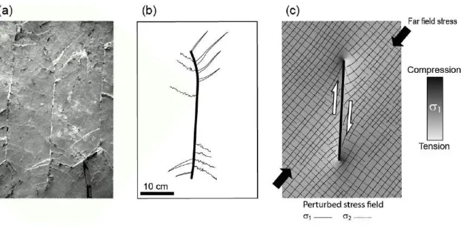
density trends). An instructive 2D illustration of the geomechanically-based methods is exposed in figure 1. It
shows a preexisting discontinuity subjected to a load that undergoes shear to create a fault. The stress is
perturbed around the fault showing both tensile (light grey) and compressive areas (dark grey). Both the
orientation of 1 (the most compressive principal stress) and 2 (the least compressive principal stress) are
8
preexisting fracture showing branch crack in least compressive areas and stylolites in most compressive
areas (Rispoli, 1981), both following the orientation of 1 and 2 respectively.
Figure 1. Comparison between (a) photo of secondary features such as tensile cracks and stylolites observed around a reactivated fracture in limestone at Les Matelles, southern France (Rispoli, 1981; Petit and Mattauer, 1995) and (b) its Interpretation of observed fractures with (c) stress perturbation computed around a single fault showing 1 intensity and orientation.
The method has been successfully applied to both outcrops and reservoirs demonstrating how
geomechanics can provide a high degree of predictability of natural fracture networks. For instance,
Homberg et al. (2004) used slip inversion and 2D discrete element method (DEM) models to confront the
observed secondary faults with the reconstructed the paleostress field. The 3D boundary element method
(BEM) has been successfully applied to model subseismic faults (Maerten, 1999; Maerten et al., 2006) in
Northern North Sea highly faulted reservoirs as well as the undetected joints in naturally fractured
carbonate reservoirs (Bourne et al., 2000) and lately, to compare differential stress magnitude trends
9
linear elastic model in Poly3D. Similarly elastic dislocation modeling have been applied to model small-scale
fault and fracture network characteristics in normal and reverse fault regimes (Dee et al., 2007).
Three key elements are essential for a complete geomechanical modeling. The first element is the
geometry of the subsurface geology called the geological model. Although this is the most important
element in geomechanical modeling, it is often oversimplified for technical and/or practical reasons.
Geological models should resemble past and/or present day natural structures as much as possible. This
includes sedimentary layers, faults, salt diapirs, cavities, folds, or any geological objects. The second element
is the stress field, which can be described as the faulting type (normal, wrench, or reverse), orientation and
magnitude of the regional or local tectonic stresses through time. This important parameter for the
geomechanical modeling is the most difficult to evaluate. While there are techniques for measuring some
components of the present day tectonic stress, it is difficult to measure past tectonic stress. These are often
partly guessed introducing very high uncertainties in the modeling. Finally, the third element is the rock
properties and mechanical behavior. This element of the geomechanical modeling is often the best
constrained. Thanks to laboratory testing, we have a fair understanding of the rock properties and behavior.
These can be extrapolated in the past using known rules on how the rock evolved (i.e. compaction, porosity,
etc.).
In this thesis I focus on the major unknown for natural fracture and present day fracture modeling,
which is the far field tectonic stress that we also call the far field boundary conditions in the geomechanical
simulation. The tectonic stress estimation is crucial for fracture modeling and existing methods advantages
and limitations should be investigated.
3. Faults and Fractures
The proposed work concentrates almost exclusively on the case where faulting is the main driver for
10
growing and active fault system, the orientation of fractures will be influenced by the regional state of stress
as well as by the perturbation near large faults.
3.1. Faults, fault systems and stress field
Faults are discontinuities of the rock along which there has been significant shear. We classify faults by
how the two rock blocks on either side of a fault move relative to each other.
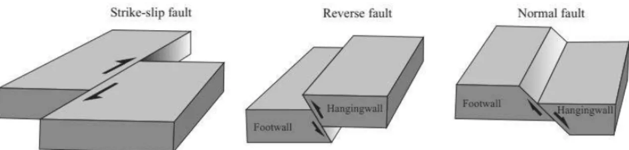
Throughout the Earth's crust, three faults types are distinguished:
(1) Normal faults, reverse faults and strike-slip faults (figure 2). Normal faults are characteristic of
regions undergoing extension (i.e. passive margins). In normal faults, the hanging wall moves downward,
relative to the footwall. Normal faults may dip at a variety of angles, but they most typically dip between
about 40° and 70°.
(2) Reverse faults are characteristic of regions of compressive shortening of the crust such as subduction
zones in active margins or newly formed mountain ranges. For reverse faults, the hanging wall moves up
relatively to the footwall. The dip of a reverse fault is generally steep.
(3) Strike-slip faults are usually sub-vertical and the rock blocks moves either or laterally with very little
vertical motion. Strike-slip faults with left-lateral motion are called 'sinistral' faults while faults undergoing
right-lateral motion are called 'dextral' faults. Each motion sense is defined by the direction of movement of
the ground on the opposite side of the fault from an observer.
Transform fault are a special class of strike-slip faults where the latter form a plate boundary, these
faults are related to offsets in spreading centers, such as mid-ocean ridges. Transform faults can also be
found in continental lithosphere transfer regions such as the San Andreas Fault in the United States. In
extensional or compressive regions a mix of normal, strike-slip and reverse faults can be found, for example,
11
faults and strike-slip faults are characteristic of a rifting extensional process. Also, faulting does not
necessarily have pure dip slip movement as described above. It is common to have some combination of
fault movements occurring, resulting in an oblique slip.
Figure 2. Schematic illustration of Strike-slip, Reverse and Normal faults. Modified from Plateau (2012)
Fault surfaces are characterized by the ratio of length to height (L / H) called shape ratio. Seismic profiles
interpretations have shown that fault geometry can be complex (Koledoye et al., 2003; Kattenhorn et al.,
2001). Fault growth is controlled by two processes: Propagation at their tip when slip accumulates, or by
fault segments coalescence in relay zones (Cartwright et al., 1996).
The analysis of their throw profile of faults (throw distribution observed along faults, from zero at the tip
line to a maximum value near its center). During propagation, faults usually accumulate throw proportionally
to their size (self-similarity) (Schilsche et al., 1996). The value of the maximum throw (Dmax) is a function of
the length of the fault (Dmax 0.03.L in average) but also of its depth (Dmax 0.1.H) (Soliva et al., 2005; Soliva
and Schultz, 2008). For a single fault, the throw profile depends on the 3D geometry of the fault (Schultz and
Fossen, 2002; Soliva et al., 2005) and is symmetrical. Numerical modeling in linear elastic media, shows
rather elliptical symmetrical curve profiles. Maximum throw versus fault length may devide from the general
trend in the case of fault interaction (Dawers and Anders, 1995; Maerten et al., 1999; Maerten, 2000;
12
The slip and orientation of the fault planes are associated to the locally perturbed far field stress
orientation. However, local stress is not necessarily identical to the far field regional stress. Indeed, faults
locally perturbate stress fields. These perturbations affect the stress magnitude and orientation related to
the displacement on a fault or a fault system.
The perturbation of the stress field is a complex phenomenon, which is the reason why it is often studied
using numerical modeling. Numerical models show that stress perturbations at the ends of isolated faults
promotes shear failure, thus controlling their propagation (growth). On a fault system, the stress drop due to
faults development has been proposed as the phenomenon that controls the fault spacing (Soliva et al.,
2006). The perturbed stress establishes the location of the fault initiation and the preferential growth of
some of them. Both intersecting faults and overlapping faults are areas where the perturbation of the stress
field is high enough to modify the throw profile of the secondary fault segments and their 3D geometry as
they propagate (Peacock and Sanderson, 1991; Willemse et al., 1996; Maerten et al., 1999; Maerten, 2000).
3D numerical studies of homogeneous elastic medium on normal fault systems showed that secondary faults
with a wide variety of orientations can be explained by stress field perturbations during the same tectonic
phase (Maerten et al., 2002; Maerten et al., 2006). The perturbation of the stress field is largely controlled
by the 3D geometry of the fault system (Willemse et al., 1996; Kattenhorn et al., 2001; Soliva et al., 2006).
3.2. Fault genesis and tectonic regimes
Triaxial mechanical rock tests highlight the development of fractures under a given state of stress. In
such tests, the applied force and displacement are known. Relationship between the fracture system and
orientation of the compressive force are obvious. From these results, it is then possible to reconstruct the
directions of the forces that generated the creation of a fault system. One of the earliest experiments was
13
Anderson (1905, 1951) was one of the first to present a clear summary of the analysis of faults systems
and vein systems in analogy with rock mechanics. The application of these concepts in structural geology
permitted to determine the direction of the principal stresses from a conjugate fracture system. To illustrate
these concepts, first, it is necessary to consider an isotropic material and a system of newly formed faults.
Consider a stress tensor 𝜎 defined in the main frame, represented by the matrix:
𝜎 = (
𝜎1 0 0
0 𝜎2 0
0 0 𝜎3
) (1)
where 𝜎1 is the maximum princpal stress, 𝜎2 the intermediate stress and 𝜎3 the minimum compressive stress
(𝜎1≥ 𝜎2≥ 𝜎3, where compression is positive). The 𝜎1 axis is the bisector angle of the acute angles of
conjugate planes, 𝜎2 corresponds to the intersection of the two planes and 𝜎3 is perpendicular to 𝜎1 and 𝜎2.
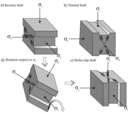
From this geometrical relationship, one can define the tectonic regimes corresponding to a normal, a
strike-slip and a reverse fault systems (Figure 2). The permutation between stress regimes can be achieved by a
14
Figure 3. Different fault types and principal stresses. (a) Reverse fault, (b) Normal fault, (c) Strike slip fault, (d) example of bloc rotation arround the principal horizontal stress 𝝈𝟏 axis. After Plateau (2012) from Angelier (1994a).
3.3. Fault reactivation
Consider a traction, denoted 𝑡⃗ (given by the Cauchy formula on the applied stress tensor 𝜎𝑟), applied at
a given point of a fault plane (Figure 4). 𝑡⃗ can be decomposed in two components: the shear stress, denoted 𝜏⃗, along the fault plane and the normal stress, denoted 𝑡⃗𝑛, normal to the fault plane (Figure 4), such as:
15
Figure 4. From traction to shear stress. The traction 𝒕⃗, the shear stress 𝝉⃗⃗ and the normal stress 𝒕⃗𝒏 are illustrated. 𝒏⃗⃗⃗ is for the
normal to the fault plane.
Using Mohr-Coulomb (1882) failure criterion and knowing the direction and magnitude of the principal
stresses, it is possible to determine the orientation of the failure plane. For example, in the case were stress
conditions are optimal (maximizing the difference between the shear stress and frictional resistance) failure
should occur when the magnitude of the shear stress 𝜏 on a plane is equal to a value of cohesion 𝜏0 added to
a coefficient of friction 𝜇 multiplied by the magnitude of the normal stress on the fault plane 𝜎𝑛. This
criterion can be written as follows:
𝜏 = 𝜎𝑛. 𝜇 + 𝜏0 (3)
Mohr’s circle allows to estimate the magnitude 𝜏 and 𝜎𝑛 at failure (Figure 5). When the circle defined by 𝜎1 and 𝜎3 is tangent to the Mohr failure envelope, which is defined by the friction angle 𝜙 with 𝜇 = tan 𝜙
and the material cohesion is 𝜏0, the stresses exceed the rock strength and failure occurs (Figure 5). The
intersecting point between the failure envelope and the Mohr circle is used to define the shear stress and
normal stress magnitudes needed to reach failure, as well as the orientation of the fracture plane (Figure 5).
16 𝜏 = 𝜎1−𝜎3 2 sin 2𝛿 (4) 𝜎𝑛 = 𝜎1+𝜎3 2 − 𝜎1−𝜎3 2 cos 2𝛿 (5)
where 𝛿 is the angle between 𝜎1 and the fault plane
Note that the example above is for optimal failure conditions, where the fracture is newly formed in an
isotropic material. This occurs when the rock material has not been deformed or faulted yet. Natural
fractures networks show more complex systems having undergone various successive failures under time
dependent variations of boundary conditions.
Figure 5. Mohr's circle representation. 𝝉𝟎 is for the cohesion, 𝝓 is the friction angle. 𝜹 is the angle between 𝝈𝟏 and the fault
plane.
3.4. Fault sliding friction
Friction is the force resisting the relative motion of solid surfaces sliding against each other. Leonardo Da
Vinci (1452-1519) pioneered in studying friction. He suggested that friction is dependent on the roughness of
the sliding material such that smoother materials will have smaller friction. Similarly, Amontons (1699)
suggested that friction was predominately due to the surface irregularities and the force required to lift the
weight pressing the surfaces together. Coulomb (1779) suggested that strength due to friction is
proportional to compressive force, although for large bodies friction it does not follow exactly this law,
which represents the second law of friction. The second law of friction is known as the Amontons-Coulomb
17
Here, in the context of geological faults reactivation, we distinguish two types of friction:
1) Material (internal) friction which is the force resisting motion between the elements strength making up
a solid material while it undergoes deformation. It is responsible to faults and fractures initiation.
2) Sliding friction which we decompose here in two type: static and dynamic (or kinetic) friction. Static
friction is the friction between two solid objects, and is independent of the time (e.g., static friction can
prevent an object from sliding along an inclined surface). The coefficient of static friction is usually
higher than the coefficient of dynamic friction. Dynamic friction occurs when two objects are moving
relative to each other. The coefficient of Dynamic friction is usually lower than the coefficient of static
friction at the end of the motion.
The static friction is also defined as an angle such as:
𝜇 = 𝑡𝑎𝑛𝜙 (6)
This formula can also be used to calculate µ from empirical measurements of the friction angle.
Byerlee’s (1978) law, which is empirically derived from experimental determination of "maximum shear
stress" on a wide range of rock types, and stating that the friction coefficients is 0.6 < 𝜇 < 0.85
(independently of the rock type) for natural sliding surfaces following the relationship (Coulomb’s friction
law):
𝜏 = 𝜇𝜎𝑛+ 𝜏0 (7)
where, 𝜏 is the shear stress of a pre-existing fracture, 𝜎𝑛 is the effective normal stress, 𝜇 the coefficient of
sliding friction, and 𝜏0 the cohesion of the rock. This relationship provides the coulomb failure
18
However, according to many authors, it is infered a significant decrease in friction as low as 0 < 𝜇 ≤ 0.3
(Zoback and Beroza, 1993; Marone, 2004; Colletini et al. 2009; Reches and Lockner, 2010; Di Toro et al.
2011) is observed for faults reactivation due to fault lubrification during earthquakes, which is much lower
than historical values (= 0.6 and = 0.85) deduced by Beyerlee, (1978).
3.5. Fractures classification and stress field
A fracture is a discontinuity in a rock mass. It can be generated when rock cohesion is lost when applied
stress exceeds the rock strength. Fractures can be observed at multiple scales, from kilometric, to
microscopic. In this study, we defined 3 natural fracture types (tension fractures, shear fractures and
stylolites) based on their development mechanism and their relationship with the orientations of the 3
principal stresses as described in Figure 6.
Figure 6. Mechanical fracture types and relationship with principal stresses. (t) Tension fracture (i.e. joint), (c), stylolite) and,
(s) Shear fracture (i.e. fault).
Tension fractures form in a direction perpendicular to the potential fracture plane reaches the tensile
strength of the rock. Tension fractures show an extension perpendicular to the fracture walls. The most
common tensile fractures are the joints but it also includes veins and dikes. Tension fractures form in a plane
19
Stylolite peaks (or anticracks or closing fractures) form with a compressive stress in a direction
perpendicular to the potential fracture plane. Stylolites are very common in carbonates but can also be
observed in clastic rocks. Compaction bands in will form in a plane perpendicular to the most compressive
principal stress 1.
Shear fractures are fractures along which the relative movement is parallel to the fracture walls. The
most common shear fractures are the faults but it also includes deformation bands. A shear fracture is one
of the two conjugate planes, oriented at acute angles on either side of the most compressive principal
stress, 1, and with opposite sense of shear direction (see Figure 6). is such that:
2 4
, (8)where is the angle of rock internal friction.
3.6. Fractures related to faulting
We are distinguishing two types of fractures related to faulting: (i) The fracture that are genetically
associated to the faulting and (ii), the fractures that are not genetically associated to the faulting. In both
cases the small scale fractures development will be affected by the heterogeneous stress field generated by
the active faulting. We therefore make the assumption that in a growing and active fault system, the
orientation of fractures will be influenced by the regional tectonic stress as well as by the perturbation of
that stress state by nearby larger faults.
3.6.1. Fracture genetically associated to faulting
Here, we consider small scale fracture development related to the faulting mechanism only. In such case
20
generated by the active fault. These fractures are generally found near the main fault and especially close to
fault tip line as shown in the two examples of Figure 7.
Figure 7: (a) Horsetail-shaped splay joints associated with a left-lateral strike-slip fault (map view) with a couple centimetres offset in sandstone, Valley of Fire State Park, Nevada (from DeJoussineau and Aydin, 2007). (b) Photograph of a strike-slip fault termination showing tail cracks (veins) in limestone at The Matelles, France.
3.6.2. Fracture not genetically associated to faulting
Natural fracturing could have many origins that are not necessarily tectonic. But in any case, natural
fracture will develop in the stress field, which could be homogeneous or heterogeneous. Here, we
concentrate solely on the assumption that the stress field is heterogeneous because of nearby active
faulting. It is important to note that very often only the fracture orientation will be affected by the
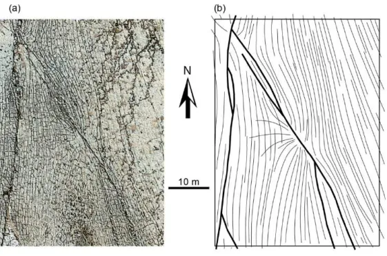
heterogeneous background stresses as shown in Figure 8 below. Here the joint development mechanism is
clearly not the faulting but faulting affects the joint development orientation. In this case faulting does not
21
Figure 8: Example from Nash Point, UK. (a) Air photo and (b) interpretation of the outcrop showing fault network (thick black lines) and associated complex pattern of joints (thin black lines). The variability of the joints pattern at Nash Point clearly shows the relationship between the strike slip faults and the development of the joints. Joints appear to have been affected, during their development, by the perturbed stress field caused by slip along faults. Here only the joint orientation seems affected by the faulting, not the density which appears constant.
Very rarely, fracture density will be affected by heterogeneous background stresses as shown in Figure
9. Here the small fault development mechanism is clearly not the main faulting but faulting affect the small
fault development density as smaller faults do not develop in the stress shadow around main faults. In this
22
Figure 9: Small faults around larger normal fault (from Ackermann and Schlische, 1997). Here, the anticlustering defining crack shields around the master faults. The shields are ellipsoidal in shape and geometrically similar to the elastic deformation fields of the master faults, and correspond to a critical stress-reduction shadow that prevented the nucleation of smaller faults in the vicinity of the master faults. You can note here that only the small fault density is affected by the main faults, not the orientation.
4. How to recover paleostresses?
Fracture modeling depends on the geological model, which is referred as the geometry of the subsurface
geology, the rock mechanical behavior, and the far field stress state at the time of formation of the fractures.
The latter parameter is often difficult to estimate especially in the context of complex structure and
polyphased tectonic history. Therefore, estimating the so called 'paleostress', which is critical for accurate
23
4.1. Paleostress estimation using Wallace & Bott type methods
The Wallace (1951) and Bott (1959) hypothesis
Fault systems are created in a given stress regime but are often later reactivated when the stress regime
has changed over time or for a different stress regime. For instance, Bergerat (1983) presented a case study
of the Rhin Graben (West European rift segment), where Eocene strike-slip faults have been reactivated as
normal faults in an Oligocene phase despite their near vertical dip. Similarly, Davatzes et al. (2003) reported
that the development of two fault sets at Chimney Rock, Utah (USA) was done during two distinct tectonic
phases, while Maerten (2000) highlighted that the slickenlines observed on the two fault sets where
produced by the same tectonic event when both fault sets were reactivated. In these two examples, the slip
data represents the last phase of slip on the faults. In such a situation, the symmetry relationship between
the newly formed conjugate fractures and the optimal principal stress cannot be applied to recover the
paleostress tensor. The only way to determine the direction of the principal stresses from slip along
reactivated faults is to introduce a relationship between the direction of shear stress and the observed slip
(slickenlines). Wallace (1951) studied the variations in the direction and magnitude of the shear stress
applied to different fracture plane orientations. He assumed that the orientation of the shear stress and slip
should be parallel and have the same direction. Bott (1959) demonstrated that the orientation of the shear
stress depends only on the orientation of the principal stresses and on a stress aspect ratio. A common
definition of the stress aspect ratio, also called stress ratio R, has been introduced by Angelier (1975) such as
:
𝑅 =(𝜎2−𝜎3)
(𝜎1−𝜎3) , with 0 < R < 1 (9)
24
The Wallace (1951) and Bott (1959) assumptions constitute the basis for inversion methods to recover
the principal stresses orientation and the stress ratio from fault plane data and slickenlines. To determine
the state of stress, it is also necessary to consider that the stress field is assumed to be homogeneous in the
rock mass, that faults are planar, that blocks are rigid, that neither stress perturbations nor block rotations
along fault surfaces occur and that the stress state is uniform and that all the measured slickenlines were
formed synchronously.
4.1.1. The stress ratio (R)
The stress aspect ratio is defined by equation (9) is between 0 and 1. When 𝑅 = 0, the magnitude of 𝜎2 is
identical to that of 𝜎3. Conversely, when 𝑅 is equal to 1 the magnitude of 𝜎2 is identical to that of 𝜎1. These
two limits present the case of a uniaxial compression and uniaxial extension, respectively. The concept of
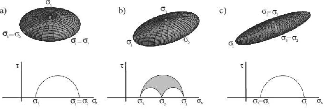
stress ellipsoid describes the stress tensor in a point, ellipsoid axes are the principal stresses 𝜎1, 𝜎2 and 𝜎3.
Figure 10 shows different ellipsoids determined from the magnitude of the principal stresses where the
magnitude of 𝜎2 relatively to 𝜎1 and 𝜎3 controls the shape of the ellipsoid.
Figure 10. Stress ellipsoids for different values of the stress ratio. Each stress ellipsoid is associated with Morh cercle illustrating the different state of stress at a given point. (a) Oblate ellipsoid with uniaxial extension (b) Triaxial ellipsoid (c) Prolate ellipsoid showing uniaxial compression. After Plateau (2012)
25
The oblate ellipsoid (Figure 10.a) shows an uniaxial extension case. The intermediate ellipsoid (Figure
10.b) shows a triaxial condition, and the prolate ellipsoid (Figure 10.c) shows an uniaxial compression. The
stress ratio can also be illustrated by the Mohr representation (Figure 5).
Depending on which of the principal stresses is vertical, v = 1, v = 2 or v = 3, the three tectonic
regimes, normal, strike-slip and reverse, can be described respectively (Anderson, 1951). The permutation of
one of the horizontal principal stress axes with the vertical one allows switching from one tectonic regime to
another. Furthermore, depending on the relative magnitudes of the intermediate principal stresses, 2, with
respect to the two other principal stresses, 1 and 3, each tectonic regime can vary continuously from radial
to axial.
4.1.2. The forward problem
It is possible to predict the orientation of slip on arbitrary fault plane based on a given stress tensor. The
stress tensor has 6 degrees of freedom. It is possible to reduce the number of unknowns since the shear
stress direction depends on the orientation of the principal stresses and 𝑅 (Bott, 1959). We can thus reduce
the tensor 𝑇 to a reduced tensor denoted 𝑇𝑟 by removing the isotropic portion of 𝑇 and a scaling factor (not
affecting the direction of 𝜏). Thus the tensor can be characterized by four parameters, which describe the
orientation of the three principal stresses (𝜎1, 𝜎2 and 𝜎3) and 𝑅 the stress ratio. This can be simplified even
further to a 2D parameter space (𝜃 is the clockwise angle between the North and the orientation of the
maximum principal horizontal stress) if we consider that at least one principal stress is vertical (Anderson,
1951).
We can thus calculate the orientation of the shear stress on a fault plane using the reduced stress
tensor. The applied stress 𝜎𝑟 is established by the Cauchy formula:
26
𝜎⃗𝑛= (𝑡⃗ . 𝑛⃗⃗)𝑛⃗⃗ (11)
The shear stress can thus be written as :
𝜏⃗ = 𝑡⃗ − 𝜎⃗𝑛 (12)
4.1.3. Stress inversion problem
Inversion problem consists in finding model parameters that better explain the observed data. In the
case of paleostress, the observed data are fault systems wth slip directions and the model is associated with
stress tensor. In the classical inversion methods, the fault system and the stress tensor are fundamentally
linked by the Wallace & Bott hypothesis. The inverse problem is defined by four parameters which are
related to the orientation of the principal stresses and the stress ratio 𝑅. The observed data are slickenlines
along fault planes. Among the inverse methods, there are two major types of algorithms to determine the
stress tensor that better fits a faults data set: grid search and least square methods.
The difference between these two types of methods can be illustrated by analogy to the best line
passing through a cloud of points in a graph (x, y). After selecting a first adjustment criterion the first
approach (Grid search method) is to try a large number of lines and determine for each of them the
correlation with the point cloud. To ensure that all the solutions are tried, one needs to systematically vary
the two parameters controlling the line (slope and intercept parameters of the line). That consists on
exploring a 2D space of the two parameters to ensure that we find the line that better adjusts to the point
cloud. Covering the full 2D space can be tedious, thus Monte Carlo method has been used in order to speed
up the searching process (Etchecopar et al, 1981 and Etchecopar, 1984). An alternative approach is to use
regression to directly determine the best fitting line. To do this, we use an equation containing the sum of
the point deviation from a general line. Using the partial differentiation, it is possible to derive a
mathematical function which expresses the slope and intercept for the line that minimizes the deviations.
27
computation time as it does not require repetitive tests. These two approaches require a criterion for
determining the best fitting stress tensor with the data. The most intuitive criterion is to use the angle 𝜔
between the calculated shear stress 𝜏 and the observed slip vector (Figure 11). It is common to determine
the stress tensor that produces the lowest 𝜔 between the model and the observed data.
Figure 11. The misfit angle between the slickenline (white lines) and the shear stress resolved to the fault plane. 𝝉 is for the shear stress and 𝝎 is for the misfit angle between the slickenline and 𝝉.
A commonly used minimization function takes the square sum of the misfit between the data and the
theoretical model. Angelier (1984) and Michael (1984) defined it as follow:
𝑀1= ∑(𝑠 − 𝜏)2 (13) 𝑘=𝐾 𝑘=1 𝑀2= ∑(𝜏𝑚𝑎𝑥𝑠 − 𝜏)2 (14) 𝑘=𝐾 𝑘=1
where 𝜏𝑚𝑎𝑥 is the maximum value of the shear stress for the considered stress tensor, and k represents each
28
Note here that 𝑀1 (Angelier 1984; Michael, 1984) and 𝑀2 (Angelier, 1990, 1991) criteria tend to
maximize 𝜏 (close to 1). These criteria are considered as hybrids since they combine both an angle criterion
and the Tresca failure criterion, where 𝜏 must be sufficient (or maximum) to generate slip on all considered
fault planes. Both the INVDIR program, created by Angelier (1990), and the inversion program created by
Micheal (1984), use these 𝑀1and 𝑀2 criteria.
Once the reduced stress tensor that minimizes the misfit between observed data and the model is
recovered, most classical inversion methods require identifying the data that are not explained by the stress
tensor. This can be measured by the angle 𝜔 (Figure 11). When 𝜔 is high (𝜔 > 30˚) the retrieved tensor
hardly explains this observed data. It may then be necessary to remove this data and to rerun an inversion
since the data set has changed.
Some more sophisticated criteria than the simple 𝜔 have been created. For example, Angelier (1990,
2002) described a ratio which takes into account 𝜏𝑚𝑎𝑥 and 𝜔. After the stress tensor has been found, a
retrospective study can help verify that it satisfies a friction law. This can be done by inspecting the data on
the Mohr (1882) representation by determining if they are below or above the frictional reactivation line
(Angelier, 1983, 1989, 1994b; Célérier, 1988; Etchecopar, 1984; Etchecopar & Mattauer 1988; Fleischmann &
Nemčok, 1991; Gephart & Forsyth, 1984). Michael (1987a) for his part developed a ‘bootstrap’ method for
sampling the data set multiple times and thus run a stress inversion on each sample.
The main difficulty of the inverse problem is related to the heterogeneity of the observed data, leading
to a multiple possible solutions.
4.1.4. Stress inversion using slip data
For the last five decades, the far field tectonic stress has been recovered through stress inversion
techniques. All commonly accepted stress inversion methods use the simple but central Wallace (1951) &
29
stress inversion (Carey and Brunier, 1974; Angelier, 1975 and 1979a; Etchecopar et al., 1981; Gephart and
Forsyth, 1984; Michael 1984; Lisle, 1992 and 1998; Yamaji, 2000; Delvaux and Sperner,2003; Celerier, 2006)
mostly using slickenlines, and quickly adapted for focal mechanisms (Ellsworth and Zhonghuai, 1980;
Carey-Gailhardis and Mercier, 1987, 1992; Gephart, 1990a, 1990b; Gephart and Forsyth, 1984; Julien and Cornet,
1987; Mercier and Carey-Gailhardis, 1989; Michael, 1987b; Vasseur et al., 1983; Angelier, 1984; 2002a,
2002b; Lund and Slunga, 1999) and calcite twinnings (Turner, 1953, 1962; Nissen, 1964; Spang, 1972;
Laurent et al., 1981, 1990; Dietrich and Song, 1984; Pfiffner and Burkhard, 1987; Lacombe and Laurent,
1996; Nemcok et al. 1999).
Many stress inversion programs have been created, these methods are either graphical inversions, like the well-known Right Dihedron method originally developed by Angelier and Mechler (1977) and improved
by Delvaux and Sperner (2003), direct inversion methods using least square minimization (Carey-Gailhardis &
Mercier, 1987; Angelier, 1991; Sperner et al., 1993) or iterative algorithms such as Monte Carlo techniques
that test a wide range of possible tensors (Etchecopar et at. 1981) or grid search methods (Gephart 1990b;
Hardcastle & Hills 1991; Unruh et at. 1996). It was also shown that the paleostress could be determined
using fracture planes which do not bear slip lines on their surface (Angelier, 1994; Dunne & Hancock, 1994;
Delvaux and Sperner, 2003).
However, the basic WB hypothesis is questionable, since Hancock (1985) and Petit (1987) studied
evidences of local stress perturbations in microstructures, while others (Twiss and Geffel, 1990; Twiss et al.,
1991; Pascal, 1998) observed block rotations along fault surfaces. Gapais et al., (2000) showed two examples
of faulted regions to illustrate the spatial variability of fault-slip data either due to local complications at the
edges of fault blocks, or to complex kinematic conditions at regional boundaries. These questions lead to ask
30
Debates have been initiated by Pollard et al. (1993) and Dupin et al. (1993) who checked the validity of
the WB assumptions by using mechanical modeling methods (i.e. taken into consideration internal
deformation of faulted blocks and local stress perturbation between faults). According to the results of
Dupin et al. (1993), the discrepancy angle between mechanical and WB predicted slickenlines reaches 47° for
intersecting faults. Pollard et al. (1993) predicted a maximum of 37° discrepancy angle for fault interaction
and a 10° misfit angle caused by fault tip geometry.
Later, Nieto-Samaniego and Alaniz-Alvarez (1997) proposed that the slickenlines should be parallel to
the intersection line and therefore could deviate from the resolved shear stress orientation. Maerten (2000)
explored the consequences of varying geometry of intersecting faults on slip directions using 3D boundary
element methods (Thomas, 1993; Maerten et al., 2014). He concluded that significant deviations are
expected close to fault intersections where the misfit angle can reach values greater than 50°. This result has
been confirmed by field observations along the Chimney Rock fault array in Utah, USA (Maerten, 2000). Xu
et al. (2013) compared observed fault striations in the San Miguelito Range with the fault interaction model
of Maerten (2000) and found that the slickenlines patterns are consistent with the geomechanical model.
The majority of the slickenlines is not parallel to the resolved shear regional stress but is consistent with
local stress perturbations caused by fault mechanical interaction.
Another approach was used by Pascal (2002) using 3D distinct element method (Cundall, 1971 and 1988)
to demonstrate that the differences between WB and mechanical models are negligible due to the
implication of the sliding friction, which reduces the misfit angle between resolved shear stress and slip
vector.
More recently, Kaven et al. (2011) pointed out that even if the stress inversion results are similar, WB
type inversions perform poorly for limited ranges of slickenline orientations when compared to their
31
any stress field anisotropy such as that arising from 3D fault geometry, can lead to a significant angular
difference between the directions of maximum shear stress and the slip direction predicted by the WB
assumptions.
Thus, studies conducted with classical stress inversion methods do not fully take into account the full
range of stress boundary conditions (i.e. stress tensor principal directions and stress ratio), fault and material
properties (i.e. friction coefficient and Poisson’s ratio ) as well as the effect of traction free Earth surface (i.e.
half-space). Methods of paleostress analysis have, by necessity, incorporated a significant degree of
flexibility with respect to the implementation of the WB assumptions.
Another concern is that, although high misfit angle are expected, no stress inversion techniques based
on the debatable WB assumptions have been tested on these specific configurations. Indeed, it has never
been shown that a low mean misfit angle correlates to a fair stress inversion result, and inversely, that a high
misfit angle correlates to an incorrect stress inversion result using the WB assumptions.
4.1.5. Stress inversion using focal mechanisms
In seismology, a fault is defined both in space (coordinates) and in time. Focal mechanisms
charasteristics depend on both the stress drop during the quake and the orientation of the stresses applied
on it. In fact, during an earthquake only a portion of fault is reactivated. Each point of the reactivated fault
surface generates a stress that is integrated during the duration of the earthquake on the reactivated fault
surface. This allows deducing the amplitude of elastic waves at a distance r from the fault. It is important to
determine this function because it is the only data that can be obtained (by seismograms). The seismic
moment (Aki & Richards, 1980) is described in the fault referential such as: