DETAILED ANALYSIS OF AN INTLSE SURFACE COLD FRONT
by JON PLOIKIN
A,.B. Cornell University
(1983) I:rGTnrEN
PUBMVITIED IN PARTIAL FDLFILLUdNT OF THIS REQUIREMENT8 FOR THE DEGREE OF
At The
ASSACUSETTS INST6TUTE OF TECNLOGY August 1985
Signature of Author .. e ... , .eo..o...e...
...-Depcrtmnt of Meteorology, 23 Auguvst 19685
Certified by Meals S6upervisor Accepted by .. .... . ... * -* Ch 6prtmentaa Comittee on Graduate Students 4
I
DE t tAMS 4T-i OF AN -NTENSE
U'ACE COLD FROjNT
by
JON PLOTKIN
Submitted to the Department of risteorology on 23 August 1965 in partial fulfillgent of the requirement for the degrse of Master of &cience.
AB6TRACT
The detailed behavior of the cold front of Jan 20-21b 1959 Is studied as it moved through Texas, From continuous traces of wind, temperature, sunshine and pressure, the frontal properties of these variables are examined.
The frontal properties of wind and temperature are affected by topography. Rough terrain is found to destroy strong gradients more quickly than flattar land. The cloud cover variations across the front are shown to contribute significantly to frontogenesis and frontolysts.
Ie confluence which is rerponsible for frontogenesis Is ob-served to cease once the front begins to move, since the convergence zone outruns the strong temperature gradient. Net diffluence in the frontal zone along with lateral mixing destroy the front once the confluence stops*
Finally, the divergence and vorticity across the front are studied, and thie rnd shift In the tangential comLponent is observed to increase as the front moves, while the shift in the normal com-ponent decreases,
Thesis Supervsor: Frederick Sanders
ACDNOWLEDGEMENT
I wish to thank Professor Frederick Sanders for his guidance
and tutelage which led to the production of this thesis. Also,
discussions with Mr. R. Tarry Willinam wore of considerable aid. My thanks also to Mr. "San" Ricel and Miss Isabelle Eole for their drafting of the difficult figures, and to Mrs. Jane
McNabb for a masterful typing job, and other technical assistance. Miss Anne Corrigan deserves special recognition for the
un-told hours she saved me with her precise plotting.
Not to be ignored, algo, is the intellectual stimulation which I received from Mr. Ken Campana and -Mr. David Tweedy.
Special appreciation must be expressed to Lance Bosart, who performed the thankless task of proofreadings, and whose unbounded
wit always provided a spiritual lift.
Lastr but certainly not least. I wish to acknowledge the moral and financial support of my wife Gail throughout zy graduate studies.
iv.
TA-BLE OF CONTENTS
14 INTRODUCTION A. Background
B. Theoretical Considerations 2
C. Objectives of this Investigation 3
D.. Theory of Frontogenesis 3
E. The Synoptic Situation 4
F. The Data S
II. FRONTAL CHARACTERISTICS OF THE METEOROLOGICAL
ELEMENTS 8
A. The TpeWrature Field 8
B. The Wind Field 13
C. Relationship Between the Temperature Drop and
the Wind Shift 16
D. The Pressure Field 18
E. Relationships of Pressure to Temperature
and Wind 19
F. Cloud and Precipitation 21
I I. FRONTOGENESIS AND FRONTOLYSIS 25
A. The Frontogenesis Equation 25
B. Confluence 2
C, Lateral Mixing 31
D, Qualitative Discussion of Frontogenesis and
Frontolysis in the Case of 20-21 Jan 1959 32
IV* DIVERGENCE AND VORTICITY 34
V. CONCLUSIONS 36
APPENDIX 1 37
APPENDIX II 40
42-1. INTRODUC TION
A. Background
Since the first exposition by the Norwegian school of the con-cept of atmospheric fronts, the attitude of meteorologists tomards fronte has gone from great enthusiasm through disappointment to the
preant air of confusion, consisting of acceptance with little
Under-standing.
The writings of Bjerknes and Solbergt are worthibile for their historical as well as their educational value. They present fronts
in conjupction with a Polar Front Theory and the formation of cyclones.
In the classical type of front, the cold air is preswmed to lie
be-neath the wm air like a wedge. The frontal surface is defined by Pietteresen (1940 , p. 274) as '"an inclined nwrow layer of transition In which the meteorological elements vary abruptly." A front Is then
the intersection of this surface with a hori.onta plane, such as the
earth's surface. The fronts of which we will speak will be tempera-ture fronts; that is, zones across which temperatempera-ture varies abruptly.
One difficulty which helped lead to the present confusion con-cerning fronts is the impreciseness of the term "varies abruptly." Current practice seems to be to extend "ahrupt" far beyond its
logi-Cal limits in analysing fronts on weather maps. Worse yet, fronts
To get a feeling for the .development of the Polar Front Theory,
one showcld first read the 1919 paper by J. Bjerknes, followed by the 1921 and 1922 papers by Bjerkies and Solberg.
2., are drawn, and g*iven the expliit nama of cold or mrL-mh ±ront, for
reasons other than nons of abrupt tempcrature variation, For esr
ample, the original theory of Bjarknaea held that all nor-convoctive
prccipitation was connected with Zrents. Tras it is now deeaed fahionaable to analyze a front Where precipitation is occurring. Again, we are awre that a temperature front is generally accoms panied by a vrind shift. Flagrantly false reasoning is used to "find" fronts by locating wind shift lines, be there teMperature
contrast or not. A similar practice for locating fronts has also
recently been applied to dpoint variation. All of this is of
course only helping to confuse the issue.
Rather than attspt to change currant practice, we shall choose to ignore the problem in a convenient mny, It we are to
learn anything about fronts, we must at least be sure our research
is done on "real" fronts, and not just regions where somene has
drawn a line on a weather map. Fortunately there exist cases of unmIstakable temperature fronts; instances where the surface ter perature may vary 25SF in a distance of, say, 40 nautical miles, along a line hundreds of miles long., Such things do occur in the atmosphere, and it is towards understanding these that synoptic
research ought to be directed. B. Theoretical Conslderations
For a very abrupt front, we might conaider that there is a zero-order discontinuity in temperaturo. For less intenoe ones, the
3.
dscontinuity ia poseFible inr the atmosphere, Irut it may be close
enough to be considered as ruch. In the cases to be considered, tUe largest gradiont of temperaturc occurs at the leading edge of the cold air, and the grtAdient decreaces in magnitude rather
regularly In the cold air, while the gradient of temperature in the marm air is always sal. In Appendix I, conditions for pressure
and geostrophio wind are derived for both zero- and first-order temperature frontm. It will be seen that for the intense fronts which we will study, the zero-order theory gives a better approxi-sation to the actual conditions,
C. 0G ve ofjelnstigton
In the following discussion it is hoped that more detailed
information can be obtained from continuous trace data than it has
hitherto been possible to aquire simply from synoptic reports. It
is hoped that somthing of value will be found from an examination
of meteorological elements over distances of a few miles, as opposed to a normal scale of tens or even hundreds of miles. Even if the.
results are not spectacular, it would seen that such an analysis is desirable from the point of view of completeness of our knowledge of fronts.
DThory of Frontogenalsi
In order to create a front there must exist som. mechanism to
pack or push together the isotherms. At the surface, where vertical
motions disappear, the equation for frontogenenis is rather
simple.
The derivation of this equatIon -is given in Appendix II. It shouldoecarefully no-,,ted that tho fial3 form-a of'A the foOenesio
eqaw-to a a air Fronts may a ppear at a particular
pofCi due to ontagknesis o parcels at that point>, or to advectir nto' the region 0iprcels rJth fronatal properties, or both, This
l dicuse m&o iully in a later secticn.
On January 20 and 21 1039, an LIton@ Surface cold ftrout Mated
through Texas, producing one-hour temperatur drop3 1n exce.s of
SOTF at some0 atations, The front formed with an east-wnst
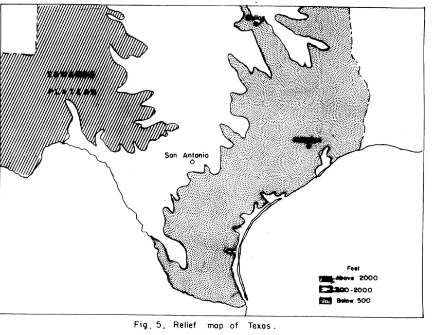
crienta-tion through northern Texas near a LBB-SPS line (sae figure I for the loations of all StatSons in Texas), thence eazt-northeactward
through Mjiouri and Illinoio, The front intensifies as a otationary front through Texas and a a ari front olsewhere, mainly through the agency of strong confiuence in the frontal zone.
Around 20 Z ona 2-1 January the front begins to move as a sharp cold fronto travoling about 25 mnot& in the scuthern portion, but less rapidly in the northeast portion. The front 2.s identifiable
until it reaches the east coatt, finally becoming oriented more outh-ouh t northnrthast The temperature contract is considerably
ameliorated as the frout noves, although the large vector wind shift, and houce the strong convergonce, is not ignificeantly decreasehd To get an idea of the magnitudes involved, conitder figure 2, ohovrng the maximum cnc-hour vector wind shifts and maximum one-hour tempera-turo changes for seted stations in Tecas Figure 2 chows that
.hroughout eastarn Texas. On the other hand, the maium one-hour
teperature change ham decreased from about 250F in the Fort Worth area to agound 10' in the Houston area. A similar effect is
ob-served along almost any path normal to the front, for example from the Louisville area to the North Carolina coast.
The questions which arise immediately are the following. My
does the front suddenly "take off" and move rapidly after remaining
stationary fo.- a considerable length of time? What causes the front
to strengthen and weaken (1 e. the temperature gradient to increase or decreaseY despite a nearly constant convergence?
In anseer to the first question we can offer only a few specula-tive comments. To the second question, a later section will be devoted, etd hopefully at least a partial answer can be given.
?irst, however, we sill be conerned with the behavior of the front in detail as it moved through Texas, western Louisiana, and wouth-western Arkansas. We will examine the fields of wind, temperature, pressure and elamd cover in the vicinity of the front. Pf. particular interest will bW the relationships among the different wea~her elements,
expecially any changes In these relationahps, or changes in the elements theniselves; and the comparison betiveen the behavior tf the front on twh smaller and larger scales.
FT_ The Dra
Besl les hourly reports from all stations, examination has been made of ay and all available continuous traces of weather elements
frou stations in the area under consideration. A few commnts are
in order concerning the accuracy and usefulness of the trace data in general; further disrussion of the particular traces will be necessary and desirable as each weather element is examined.
The principal difficulty in working with the trace data was found to be in determining the precise time on each trace, due to
a lack of adequate time cheeks4 In many cases no time cheeks at
all have been made; in a few oases the exact time is written on the trace at intervals; in the majority of aases, however, only nominal time checks are made at six-hourly intervals; that is, words such as 6 h or 12 Z are written, or possibly only a mark i. made. In these cases, it is assumed that the time check is made within the ten minutes prior to the nominal hour. However, since we bill be interested in changes over times of the order of a minute or two,
an attempt must be made to increase this accuracy in time.
First, it is noted that the accuracy of a single trace during the interval of interest is much greater than the absolute accuracy in time. Since the entire period of interest at any one station is rarely more than a few hours, and since the error of the trace is probably of the order of a minute or less in that amount of tine, each trace by itself will offer the accuracy we desire.
Second, it is possible in many cases to check traces against
hourly reports and remarks thereon. For example, often the precise time of a wind shift or a pressure Jmp is reported. It no diredt
7.
yield additional accuracy. Finally, when there is no alternative,
At Will be assumed that six-hourly checke are made at five minutis before the hour.
A second. and perhaps even more irritating inadequacy arose when it came to comparing the relationships among various elements.
That vas that no station had instruments for recording wvery element oontirmously. Thus the comparisons must be made piecemeal. and the pieces thus obtained fitted together. Fortunately, complete trace data have been obtained for two stations at the time of passage of
a similarly intense cold front In March of 1965, and these data
!1. FRONTAL CHARACTERISTICS OF THE ETEOROLOGICAL ELEMENTS
A. The Te *rature Field
In figure 3 are exhibited all of the pertinent temperature data
near the time of front passage, Dashed lines are isopleths of maximum one-hour temperature drop, It is Imediately obvious that
this quantity decreases as the front moves southeastard* Perhaps
of equal importnce, however, is the considerable distance the front
travels before the maximum one-hour drop is reduced from 25 to 20 degrees, and more particularly, the region in which this occurs.
Figure. also contains a set of solid lines which divide the area into four rather arbitrary regions, denoted by roma numerals. To be sure, the transition regions are not clearly defined, and the
transition is not a sharp one; yet each region exibits a certain charateristic behavior in the temperature dropk Figure 4 is a
re-production of a representative trace from each region. We will attempt to show that the topography of the area plays a prominent part in determining the characteristics of the temperature traces.
In region 1, the drop is sudden, rapid and large (greater than lSF in one hour), As was mentioned, the magnitude of the drop de-creases southeastward, but the rapidity of the drop is undiminished.
Region II lies to thee west of region I. Here the entire tempera-ture drop took more than one hour to accomplish. Rather than a sudden rapid drop, the fall was moderately large, and lasted tio or three
hours instead of ten or twenty minutes.
In region Ill the drop is sharp, but rather small, generally around 10 degrees. In the eastern portion this may be considered
a natural extension to the southeast of the trend in region 1.
However, the osatern portion hardly represents a continuation of region II.
In the extreme south, region IV, the sharp drop has disappeared; the entire fall is less than 15*. in comparison with the larger total drops in region II. In fact, here ve no longer have an intense cold front*
Those regions and their characteristics may be influenced by three effects. First, sunrise and sunset occur at very Inopportune times as far as we are concerned* Sunset of the 20th found the front between MW and FWH; the 80 difference in maximum one-hour temperature drop between these two stations Is partially explained
by the radiational cooling which occurred at Fort Worth In that
first hour after sunset. Again, the sun was juAst rising as the front came through -egion IV. It Is easily seen that a slower drop in temperature would occur once the sun bad risen.
Perhaps more important along the coast, however, is the effect
of the Gulf of Mexico. South to southeast winds produced low clouds
and drizzle in advance of the front, which kept the temperature lower to start with. Thus, the teMperature drop could not be so extreme In magnitude.
10 that uch of region I V sre the temperature drop was nearly con-Stant is coastal p1an* Observe too,that region 11 covers the Edwards Plateau and highlands to the northwest. The suggestion
here is that the rough terrain has a destructive effect on the front0 at least inofar as the sharpness of the teperature drop
Is cofcerned. The evidence Is particularly strong aheni we note
?tnk a sharp temperature drop Is again observed to the southeast
of region IIt, in the lower ground of region 111. Evidently the
frontal confluence is sufficient to restore the near zero-order discontinuity once the front is over less rugged terrain.
Why PRI received a sharp drop Is not quite clear, but we can sug-gost that AIt may have to do with being in the Rio Orande valley
Lack of data in the area makes further conclusions impossible.
The data recorded in figure 2 are of three types. First, hourly reports0 hiVch are clearly of little use in eamiing detailed
frontal structure since rarely, it every is a temperature observa-tion taken between hours.' second0 thermograph traces are adequate
to define the general shape of the temperature curve. However, the time saee is such that Shan the temperature is changing rapidly, changes cannot be measured accurately for time Intervals shorter
than about 20 minutes6 as can be seen from MAF's trace in figure 4(b). Fortunately another type of temperature trace is available* Telepsy-chrometer traces were obtained from SAT, ACF, BRO, and LKC, Portions
of the first three of these traces around the time of frontal passage
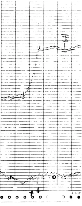
114 are shown in figure 4; LKC Io trace Is reproduced in figure 6,
AC7 Is typical of region l, and LKC is on the southern edge of that region, while SAT is just across into region lIs northern part. The differences among these three traces are mainly in the magnitude of the drop; the sharpness is present in all three* Rowever, BMos trace is of a different character, with only a gradual fall. Notice, moreover, that the magnitude of the entire drop is about the Sam' at BRD as at SAT.
The traces at ACF and LEC are believed to be typical for a strong front, The most rapid drop occurs in the first few minutes after the
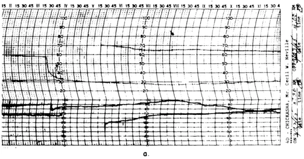
front passage, which we will define as the moment the temperature begins to fall significantly. Thereafter the rate of drop decreases with time and finally the trace levels off, Coparing with the front of March
23, 1965, we find strikingly. similar microthermograph traces for
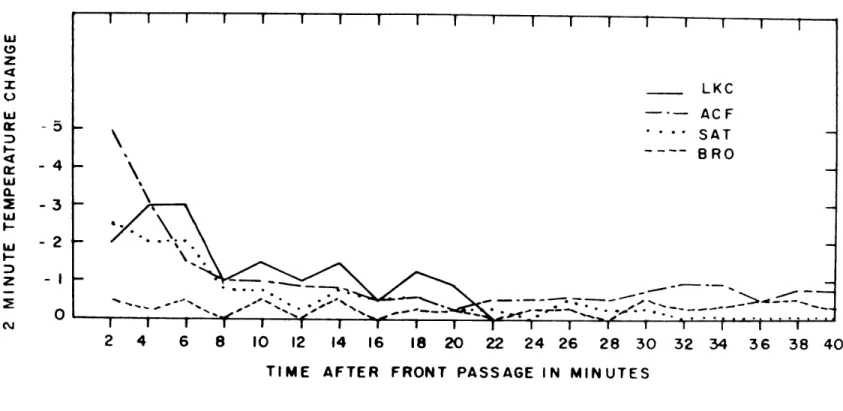
Chickasha and Norman, Oklahoma. These traces are shown in figure 7. The talepsychrometer makes a mark every two minutes. Thus we have a fairly accurate measure of two-minute tmperature changes at the four stations for which we have such traces. These two-minute
tem-perature changes are plotted as a function of time after front passage in figure 8. Since ACF and LCC lie on a line nearly normal to the
front, we can consider differences between them to be a result of changes
in the character of a particular portion of the front, One noticeable difference i. that the large drop of the first two minutes at ACY is
12,. randon ortor or instrumental lags it is terpting to say that the same sort of thIng happened to a larger entent betiseen SAT and BOQ the initial 2-1/2- drop in tvo minutes at SAT requiring nearly 20 minutes to occur at BRO. However, the SAT-BRO line makes an angle of about 20* with the normal to the front. Hence the portion of
front passing BRO is not the same portion that passied SAT. Neither would It be proper to assume constant conditions along the front. For excample, the front passes LKC and BRO at about the sae time, but clearly different conditions ctist. In spite of these diffi-culties, it does appear proper to conclude that somehow the
tempera-ture gradient is decreased as the front proceeds, especially the large, nearly instantaneous drop occurring imediately at the front.
Thus far we have tacitly assumed that the conversion from OT/) t to OT/fy, that is from temporal to spatial coordinates, is equivalent at all stations. This depends on the front's having a constant rate
of motion, In actuality the front accelerates from about 18 knots
in the Fort Worth area to near 30 knots on the southeastern coast. It is seen that this serves to increase the observed differences when put in spatial terms, and thus to strengthen the conclusions.
Using a frontal speed of 18 knots at ACF, the makimum trw-minute
temperature drop of 50F converts to a spatial gradient of 8* per nautical mile. This is decreased to a maximum twoaminute droY of 30 at LKC,
or, using a frontal speed of 30 knots, to a spatial gradient of 30
13.
B. The Wind Field
The frontal wind shift in this case, when examined closely, turned out not to be a simple phenonenon. In general, the wind shift
con-sisted of two separate events, the shift in direction snd an increase in speed. Theme two events need not always, and indeed, in our case did not usually coincide.
A shift in direction is generally considered by most people to be
the essence of a wind shift. Yet a change in speed can be an equally
significant vector shift; in fact, we ill find that in many enses the increase in speed was a more important phenomenon for frontal considerations. To be sure, a decrease in wind speed also qualifies as a wind shift, and this was the case at RESE; however, all other
stations recorded an increase for the wind speed shift for this front. The pertinent data for all stations for which we have wind recorder or wind gust traces are recorded in figure 9. In addition, the time of the start of the temperature drop at several stations is noted for convenience, and some additional hourly and triple register wind data are added where needed.
The stations to the north and east of the solid line on figure 9 (region A) all receive both the direction and speed shifts within a few minutes. At EMD, the speed shift is no longer rapid, requiring about 30 ainutes to be accomplished, and at its conclusion a small increase in speed occurs. At all the other stations in region A, both speed and direction shifts are large.
14.
Hopefully FWH, WAO and SFD lie on a line near enough to the norml
to the front so that we can consider the same portion of the front to have passed each. Figure 10 shows isogons and isotache at these
three stations around the time of the front passage. The result is strikingly similar to that obtained for temperature in that the time rate of change of both wind direction and speed are reduced as the front moves southeastward. This implies, as we saw, that the spatial gradients are reduced even more due to the acceleration of the front.
All of the stations in region B receive the speed shift substantially later than the direction shift. To the northwest, RES, which is just south of where the front forms has, as we noted earlier, a reduction in wind speed which approximately. accompanies the direction shift. This station represents no contradiction to our theory that the single convergence lina splits into a direction shift, followed by an increg
in speed. The mechanism is as follows: the convergence which breaks
ahead is a shift from southerly to light northerly; the second shift is from light to moderate northerly. At all stations except REE, the
speed of the south wind is less than that of the northerly wind in the cold air. Thus when the shifts are iMAIltneous, the result is a decrease in speed. The fact that REE, probably for reasons of topog-raphy, has a stronger south wind than thbefinal norh wind is of little consequence. But the result is that when the two shifts are
superiMposed4 1EE has a decrease in wind speed.
15.
his speed shift by several hours, all other direction shifts preceding speed shifts by less than one hour. The DYS trace is corraborated by
hourly reports from both DYS and ABI, which experienced a similar occurrttce. BWD, some 60 miles southeast of DY, received both shifts
within an hour. The noning of all this In not entirely clear. To be sure, the convergence sone (direction shift) which passed DYS at
1305 C never reached BWD (unless it dawdled terribly, which is highly
unlikely)* Here is one instance at least where the convergence con-neoted with the direction shift is a more transient feature than the
front itselt. We shall presently produce more evidence to the effect that the speed shift represents the "real" frontal convergence.
It has been suggested to neL that Abilene's wind direction shift represents a change of air mass and is thus not the same hind of thing as the "forerunners" which occurred farther south. In favor of this idea it can be pointed out that no stations lie near Abilene to this north, and that an oscillation in the isotherms of the kind re-quired to bring the front south of Abilene can be supported in hourly temperature data. Furthermore, the oscillation it somewhat supported
by the existence of a pressure wave traveling along the front. In
addi-tion, a drop in temperature of a couple of degrees is noted in the hour the shift occurs, and the dovpoint drops 40 at ABI and g* at DYS.
On the other hand it should be noted that preceding the front passage,
18. BW experiences a depoint drop of 100 in two hours, with a shift in
iind xony from south-southwest to southwest. At this point our argu-Mont becomes fundamenGtally semantic. It seems highly probable that Abilene's vdnd directien shift is a hind of forerunner. It was uffi-Ciently powerful to create a very small tmpoerature "front" and a moderate doopoint front. The convergence line petered out, but some of its effects carried on to drop BWD1's dewpoint. The point is that this forerunner traveled over air with sufficient gradients of tempera-ture and deopoint so that frontal characteristics could develop. In the cass farther outh the forerunner aets upon air with no siguif1-cant gradient of temperature or dewpoint, so no frontogenesis can occur. C. Relatonship between the Temperature Drog and the Wind Shift
So far we have not mentioned how the time of the temperature drop
relates to the wind shift. From figure 9 we se that everywhere reasonable data exist, the temperature drop accompanies or closely follows the wind
speed shift. In no case does any significant temperature drop occur
when there is a direction shift which is followed by a speed shift. Thus it is the convergence associated with the shift in wind speed which in
this case is associated with the frontal temperature discontinuity. The
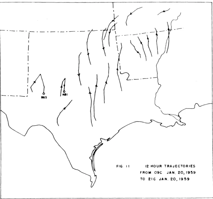
question arises, whence cometh the wind direction shift? To answer. this question, let us look a little more closely at exactly what is happening. Figure 11 shows 12-hour trajectories for the period 06 C Jan 20 to 18 C Jan 20. It is clear that the air which reaches ABI and
17. trajectories begin and and on the some side of the front. Hence the wind direction shift would be expected to accompany the temperature drop in region A. In region B, however, the convergence -line asso-elated with the wind direction shift somehow outruns the told air.
As a result, warm air is trapped on the north side of the wind
direc-tion shift, and thus no significant temperature drop accompanies this shift. Meanwhile the cold front (the temperature front) may or may not be left with a convergence zone. However, geostrophic theory
(see Appendix IA) requires that there be cyclonic shear in the
geo-strophic wind across the front, at least in the case of sero-order temperature discontinuity.
The following model can accoumt easily for both the required goo-strophic shear and the observed convergence. Suppose, as in figure 12(a), that the geostrophic wind Is from the +-direction. Assume that the gradient is stronger on the cold side than the warm, so that cyclonic shear exists. Now if any cross-isobar flow exists, which surely must be the case at the surface, the actual wind will blow as in figure 12(b). It is obvious that in this case we will have a con-vergence line along the front.
An alternate explanation of the wind speed shift may be mentioned at this time. If there were no change of pressure gradient across the
temperature discontinuity, a wind increase might be obtained due to differences in vertical mixing. If the cold air is descending rapidly,
I*
mechanism and the one outlined above are active at the front.
Recall now that wind region A corresponds to temperature region !,
and that this region did not experience as repid frontolysis as re-gions II and III farthor west* Since at least part of the frontal
convergence in wind regiQn B outruns the frontal zone, thus deoreasing the confluence; and since we believe confluence to be the primary frontogenetical force, it is not unexpected that frontolysis should proced more rapidly in region B thean In region A.
D_.MThe Presure ield
In general, the pressure field behaved such as we ould expect. The only unusual tendency Tas for the lowest pressure to be reached in the warm air. The pressure generally leveled off or even rose slightly in the warm air at most stations. However, this is generally observed to
be the rule for this area when a front is passing. As the front passes, ,he pressure suffers a discontinuity. In many cases, this seems to be almost a zero-order discontinuity, hiile in others it. appears more as a first-order discontinuity which is expected from the geostrophic theory of zero-order temperature fronts. At any rate the initial very rapid
rise is followed by a slower, but still rapid rise, usually averaging two to three millibars per hour for several hours. Junction's trace
is typical and is shown in figure 13.
It was hoped that some relation could be obtained between frontal behavior and waves on the frout. However, no identifiable center of lowest pressure formed until it was out of the region of interest. It
may still be possible to trace pressure perturbations through pres-sure changes. For the Most part, iowever, the pressure remained lower to the southwast, with an inverted trough to the northeast. The eventual low center forms in this trough in Arkansas, Figure 16 shows the pressure pattern at 21 C the 20th.
E, Relationshi ofP Wind
In a previous section we showed evidence that the wind shift
phenomenon becomes a double-barreled affair, especially in the southern and western portions of Texas. Also, we found that the temperature
drop accompanies the second shift, which takes the form of a sudden increase in speed* We will be interested in knowing where the pressure discontinuity occurs in relation to the two wind shifts. We are ham-pered in this effort by the lack of simultaneous wind, temperature and pressure data at most stations, and by the lack of good time checks on the barograms. The time of the pressure discontinuity has been entered on fIgure 11 for six stations.
In the northeast part of the state, where the wind shift and tem-perature drop were simultaneous within the accuracy of our records, ACF recorded a pressure rise starting within two minutes of the start of the wind shift and temperature falls This Is not a surprising result, and probably represents the conditions at any very strong front.
At three stations, EFD, BRO and NIB the prASure rise approximately accompanies the first wind discontinuity, the direction shift. At EFD this shift is slow, beginning at 0300 C, which is when the pressure begins
20. to rise rapidly. A small gust occurs at about 0400 C, and the
tem-perature begins to-drop. At NIR and BRO the situation is more clear-cut, with a sharp wind direction shift accompanied y the pressure
jump, then followed after about 30 minutes by a wind gust and at least in the
case
of Brovnsville, Aere we have a telepsychroaeter trace, a temperature fall.The results of the trace data at BRO, NIR and MD is corroborated by hourly reports from most of those stations which reported pressure
jumps and wind shifts, and at which the individual hours occurred at times which allowed us to determine whether there was a double wind
shift, and it so, heen the temperature began to drop relative to the wind shifts. At CRP and COT the succession of events was similar to BROO aith the pressure jump and wind direction shift occurring
simul-tanecusly, followed in about 30 minutes by a temperature drop and wind
speed shift.
Unfortunately, three stations do not fit the general picture. ABI got his pressure jump along with his wind gust. The direction shift was accompanied by no hint of a disturbance on the pressure trace. We have already pointed out that .the forerunner which passed ABI and DYS was different from the one farther south and this is just one more manifestation of that difference.
The San Antonio area presents a more difficult problem. Here the wind shifts appear to be of the type that occurred elsewhere in wind region B. However, a closer look shows us that at the time of the
21. wind direction shift around San Antonio the speed was nearly nil, and in any oase not over 3 knots. Thus the convergence involved must be small and w need not expect a pressure jump. A little later we will
see how the convergence in the San Antenio area compars to that
elsewhere.
The hourly reports from Junction suggest something similar to San Antonio. It is impossible to tell just how light the wind became when
the direction shifted, but under 3 knots is very likely. Thus it seems
4
that only to the south and east of San Antonio do we get a clear
asso-elation of the wind direction shift with the pressure jump, while the
wind gust is associated with the temperature front. To the north, the wind gust, teoperature drop and pressure jump appear to be' simultaneous.
S.
Clou
A PrecinitatiM &on
Although not important in the consideration of this front on a time scale of the order of minutes (corresponding to a distance scale of order of a few miles), the field of cloud and precipitation seemed to have some effect on a larger scale frontogenesis and frontolysis.
It was hoped that use could be made of sunshine records on the
triple register charts. Unfortunately their value is much deleted by the fact that the front moved through the region under study almost entirely at night. Nevertheless, some points can be made with the
help of hourly data. The pertinent information from hourlies and
sun-shine records is given in figures 15(a) and (b). On the sunshine records, the criterion which governs whether sunshine Is recorded is not a rigid
22.
Go
Q.iGerally the instruaent shaould be set so that it barely records sunwhin when the dish of the sun is plainly visible through the cloud. At any rate, the quality of the traces is sufficiently good for our
purpetI as.
wgure 15(a) Is divided into thre areas; area N, comprising nearly
thi northern half of Texas, shows generally scattered to broken con-u ions before the front pasage. Within a few hours after the pas-age, conditions have become overcast, with various forms of precipi-tation including rain, snow, uleet, drizzle and freezing rain or
driznle. We can corroborate at least part of this story by noting that
DAL received continuous sunshine, and ABI had only a small Interruption
in sunshine betwen noon and sundown of the 20th. If we can construe
this to imply more favorable insolational heating conditions in the warm air than In the cold, we might expect a contribution to fronto-genesis from the diabatic heating term.
The major intensification of the front occurred during the daytime hours of the 20th. In the cold air, SPS and CDS reported continually overcast or obscured sky, with much fog and precipitation. The tow-peraturos at these stations, and others in the cold air, fell during
the a th, and this may be directly attributed to advection of colder air from the north. In the warm air, however, at least at some
dis-tane from the forming front, somrie of the cloudiness burned off by ntd0-morning to allow a fair amount of heating. To prove that the
23
obzesve that the mAmum temperature around Dallas ma in the- middle seventies. Yet at sunris that morning, no 700 reading was to be found in the entire state.
In area S, the southeast coast, the story was almost entirely re-versed. Here fog and drizzle persisted in the warm air, and the front was generally accompanied by a shower* But within a few hours skies
had mostly cleared, and since it was now daytime, sunshine was abundant. At PAH and GLS, full sunshine had begun by 11 o'clock.
One might think that during the night region S would experience the
reverse .effect from region N; that is, radiational cooling in the cold air strengthening the front from the cold side. Indeed, this might have had something to do with. the surprisingly sheap teperature drop at HOU* However, we already noted that the water trajectories of the warm air produced a frontolytical effect, hiich probably more than canceled any radiational frontogenesis, and dmen the sun rose the radiational effect also became frontolytical. Thus we have marked frontolysis in the temperature field on region S.
Region C, the rest of the southern half of Texas, shows little varia-tion in cloud condivaria-tion across the front. Since marked frontolysis
occurred in the western portion of this area, we must look for some other explanation besides radiation.
It may be remarked that the effects of radiation will oscillate from day to night, and no cumulative effect is to be noticed on a front which
is stationary for some days. However, it should be pointed out that
24. and that this oiculd 2mply a proforrad time of day for frontogenesis
to occur, day or night, depending on variations in sky conditions across
the front.
Furthermore, our caSe is an example where the heating and cooling effects would not be expected to be equal. The warm air was hmid ewough to produce cloudiness during the evening, thus cutting off some of the outgoing radiation. It is also possible to Imagine that diabatic fror tagensais could occur on a parcel of air which might be transported to an area hore, despite silar sky conditions, radiation conditions
might be quite different due to the varying nature of underlying terrain. In our case: let us assume that no radiation occurred in the cold air. and that there was no temporature advection in the warm air. A good approgimation to the amount ofC diabatic heating in the warm air would probably be gtven by the difference between the morning minimum and
afternoon maximum temperatures, whIch is around 10F. If this represents
the diabatiC fr.ontogentical effect across the front, then we have an
offect of about 25% of the entire frontal gradient. Clearly, then, it is
a very crudi appraimation to neglect the diabatic heating term in the
25j.
III. FRONTOGENESIS AND FROMNTLYSIS
A. The Frontogenesis Eauation
Equation (1) shows that tlm rate of frontogenesis is given by three terms:
(1) }).
For the derivation of this equation and a discussion of the meaning of its terms, the reader is referred to Appendix II.
The confluence term, is quite obviously strongly frontogenetical along the front under study, since a con-vergence zone coincides with the zone of large temperature gradient. For our purposes it will be sufficiently accurate to replace poten-tial temperature, &, by actual temperature, T. at the surface, since we will be concerned witi horizontal distances of the order of tens of miles, and thus no very large land elevation differences are in-volved.
The twisting term, -, vanishes at the surface due to the disappearance of vertical velocity w* Since we will be concerned only with surface frontogenesis, this term will be dropped.
The final term .of (1) is the diabatic heating term, which we pre-viously., found to be substantial at times. However, the confluence appears
to predominate, and we shall consider now the term - alone.
2-.
B, Cclnflunce
One way to approach the confluence is to try to measure it
directly froa heurly maps. The analysis oZ T and v is of course
cow-pletely aorarate only at each station. The tfeld of temperature is
fairly regular, ard 8T/By is probably quite accurate at a grid distanoe
of SO ICiloreters. Howver, v Is muth iore likely to fluctuate. The
product will be inaccurate ver 30 kilometers if either
T1 or v dparts markedly froa a linear variation, tnd particularly so i v/ay or OT/8y Changes sign.
Consider the sle illustrated in figure 16 Using a grid dis-tance of 50 kilometers in figure 16(a we would calculate that
or about 25- F over 50 Ica in 3 hurM a large confluence indeed. But
now consider that t have a third data point. C, Midway between A and B
as in fgure 10(b) Now using a 25 km grid distance we calculate that
T/6Iy fro A to C is zero, and ?8v/y from C to U is aro. Thus there is no not confluence betwen A and Pa, which is a far different result than we obtained abvue We 7412 fnd that such an effect as this is
actual1y lf operation In our frontal case.
As lotnn as the wind shift line eoinoides with the start of the tem-perature d.eop, wa don't have to worry too MAch about difficulties of the type deeoribal aborvea Of course minox irregularites will occur; but the major area of lsrge tov/ay wil correctly be superimposed on
Figure 17 shoVs the conflusnee field as computed from hourly reports at 21 C the 20th. As expected, the values are very large in
a narrow strip along the Zront. It it Important to realize that these values are those which obtain on individual parcels of air, In addi-tion, of cuse, parcels are being advected. It Is Interesting to note that it we consider the convergence sono to be stationary, so that
the confluence is continually esaurring on the saMe "parcels", it would
be easy to produce a temperature gradient of 25*/50 km In a time of only three hours, even starting from a relatively weak temperature
gradient. This of course asMres that only confluencs Is acting. In
actuality, frontogenesis does occur quite rapidly in many ases; but perhaps more pum2ling is the fact that despite the continuance of what
seems to be strong confluence, our front actually suffers frontolysis once It begins to move.
To increase our resolution to dstances less than 50 km, we can use
continuous records and convort from temporal to apatial coordinates as before# This method assumen (1) that we know the speed of tho front fairly accurately, (2) that the front moves normal to the isotherms, and
(3) that conditions near the front are not significantly changed In the
period of time under consideration. For a front moving at 25 knots, this latter condition is likely satisfied since all of the interesting
changes occur in a time of less than one hour. Conditions (1) and (2) will be assumed to be sufficiently oatisfied.
The first problem we face is that no station has simultaneous records of wind and temperature. The beat we can do Is to use etations close
28. together, one of Wth records tmperature and the other wind. Sinee the behavior of the tezparatur4 is reasonably Similar at stations Close together, we can legitimately apply the tewperatura trace at one sta-tion to another stasta-tion a few miles away. The only problem is to
acwately determine the oorrespoading tire scale.
In the Fort Worth area we have a telepsychrometer trace from ACF aid a wind trace from FWH, Frm the telopsychroneter trace, the time
of the beginning ot the temperature drop Is 1841 C. 'The hourly reports
claim a frontal passage ocurred at 1042 C, We refuse to admit that the preolpitous temperaturo drop could begin before the wind shifted (which is likely what the hourlies mean by a front passage). Thus one or the other of the times Is off by at least one minute. It is
likely from the position of Fort Worth relative to the front's
be-drop
havior, that the wind shift and temperature/occur at about the same time (reoll that Forth Worth Is In temperature region I).
Using the ACF tIme scale, we have adjusted the time on the FV wind
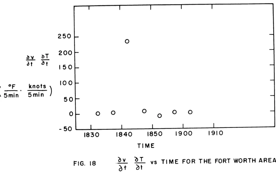
trace so that the beginiaug of the wind shift occurs at 1841 C. Com-putatIons of v were made at five-minute intervala, and
was omputed for each fiv-minuto interval, Figure 18 Is a graph plotted against time, with -alues for each flvr
minute interval plotted at the midpoint of the Interval.
As we expect, a huge value of Is obtained at
the front. If we use 20 knots for the Speed of the front at Fort
Worth, then five Minutes converts to about 17 nautical miles, and the units of tigure 18 convert coaveiently to OF/ram./3 hr. It is no
29. surprise that with such a confluence, a near neir-rder temperaturo discontinuity is able to occur.
The second locatIon where trace data are sufficient to allow con-fluence measurements is in the San Antonio area. In this case the
rind trace is from SEW, and the temperature trace from SAT. Here there is a sIgnifleant time lag between the wind shift and the start of the rapid tamperature drop9 To pinpoint the exact time of the lag
is not possible; however we can obtain reasonable limits by examining hourly data.
SAT reports that his wind has shifted to NNW 22 + 25 at 2332 C,
although no time for the shift is givan* Since he does report a pres-sure jump at that time, howvrer, It is likely also the time of the wind shift, at least within a very few minutes. The hourly tesperatures
given at SAT are 64 at 2258 C and 85 at 2358 C. Matching these to the telepsychrometor trace, this pinpoints the temperature drop at 2347 C (and also indicates that the telepasychrometer time scale Is 10 minutes in error). The lag thus computed is 18 n-ues,
Further chocking hoews that at nearby RND, a front passage (meaning wind shift) is reported at 2340 C. At 2368 C the hourly temperature is reported as 63t a drop of only two degrees from the previous hour.,
Presuming that RNtD had a temperatue trace similar to SAT, the tempera-ture drop could not have started bvfore 2357 C, a lag of at least 17 minutes. The conclwich must then be that the time lag between ind
shift and temperature drop in the San Antonio area was between 15 and 20 minutes.
30. Figures 19 and 20 shoW the fiVe-Minute changesof T and v at SAT and SKF respectively* We can see that the most active portion of the wind shift requires only about five dste or les to occur. The init-ial five-mIniite chnge of -20 to followed by a +8 in the next five minutes, where positive values Indicata divrgenic. Thereafter
a lesser convergen&ce is followed by divergenco of nearly equal magnitude.
It may be argued that these zones of divergence and convergeanoe, and those which foll.ow, are siMply a reault of random gustiness in the wind. Nevertheless, it is clear that if the gusta are not randomly super-imposed upon the temperature field, then non-random frontogenetical
effects can be expectedv in particular,. this may be one of the mechanisma operating in the frontolysia of moving front.
In the San Antonio case, figurea 21 and 22 show the confluence com"
puted from the 6T/at and Ov/Ot values of figures19 and 20 at 15 and 20 minutes' lag respectively. For 15 minutes' lagi sme fair confluence is produced by concurrence of the -5 BT/Ot with the -3 Ov/Pt, but at 20 minutes' lag,, no outstanding confluence is evident; in fact, for 20 minutes' lag, the sum of the confluences for the first 30 minutes after
the temperature starts to drop is -2, or very slight diffluene for the period.
Of course we must point out again that the preceding computations
were made with data from two different stations. Local effects, par-tieulwsiyin the wind, may be a misleading factor in any Individual case.
An examination of the correlation between LYT/6t and Ov/t for a large
frontolysis or frotogeneaia in moving frontr; hopefully trace data
will soon be available for such an invstigatiom. Presently we can
state that the wind shifzt definitely outrun's the strong temperature gradient in some regions. In others, it Is posible, Indeed likely,
that the wind shift gets only slightly ahead of the teiperature drop. However, if the shift IS very rapid, the confluence ill immediately cease. Then turbulont procemses, either of the type suggested above or on a saller scale, will become the primary factor In frontelys..
The method of frontolyols outlined above depends on a correlation boteen OT/by and O/y. Lateral miing of a random nature will also.
be acting, and this may turn out to be the more important type of
-tur-bulance. The classical equation for heat transport by horizontal
dI-fusion isnIZ
I
where A is the coefficient of lateral diffusion. If the turbulent
motion in the atmosphere iere isotropic, then the coefficIents of di'-fusion wuld be the same in all directions. We cond then use the
estImates for the vertical diffusion coefficient which ranges from
103to I e 2/s Let us use the larger value, and the largest value om can tad. At ACF %v saw that LT/Oy goes from Q*F/hm
just on the varm sde of the front to approximlately 4*F/mu just behind
32.
this by 104cm /seo, we get BT/Ot = 4 x 10 OF/sec, or about
4 x 10⁻² OF/3 hr, very small indeed.
Unfortunately in a fluid with stable stratification, such as the
atmosphere, the turbulent motion is anisotropic. Estimates of the
coefficient of lateral diffusion have been made as high as 103 higher than those for the vertical coefficient1. Using A = 10 cm2/see, and uinglo F/km, ony 25% of the value we used before, we
find ()T/Ot = 100F/3 hr. It is clear that with this value of A, even the strongest front uvld be obliterated in a matter of hours.
The correct value. of A is likely in the range 105 to 10 Gn 2/eet, and the lateral mixing likely has an effect an the front. Whether this type of diffusion or the systematic type outlined previously is the more important is impossible to tell at present. Probably both are at work.
D.
Qalitative
Discussion of Frontogenesis and Fiontolysis in theCase of 20-21. Jan 1959
A qualitative discussion of the frontogenetlcal process in this case is now in order. To begin, a broad region of modest temperature
gradient is present with mostly easterly winds throughout the colder portion and southerly winds in the warmer sector. As the southerly winds reach the convergence line, the warm air is lifted above the cooler air to the north. Due to moderating effects of water to the
south, and the fact that little temperature gradient existed some
33,
distance south of the front to begin vith, the area south of the oon-vergence line becomes relatively constant in temperature, except for
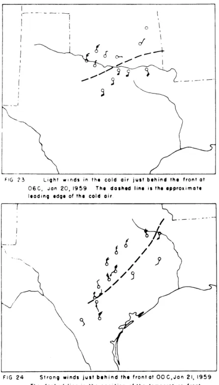
diurnal trends, North of the front, vinds slowly turn mre northerly, but remain light near the convergence line. Since the winds just north of the convergence line pretty auch control the motion of the front,1
it remains nearly stationary. This contention of light winds near the
convergence line is supported by hourly maps, one of which is shown
In figure 23.
Now confluence has been set up just north of the convergence line,
which can now be called the front. The front moves only very slowly as a large temperature gradient is produced on its northern side. The winds near the front in the cold air increase and the front begins to move; at first the convergence line and the leading edge of the cold air move at the same speedbut later the cold air begins to log.
At this point turbulent motions, particularly over rough terrain, are beginning to have a frontolytical effect. In addition, there has ceased to be confluence in the cold air, since the wind at its leading edge has
become at least as strong as the winds deeper in the cold air. In support
of this statement, figure 24 is presented. As we have shown, it is
pos-sible that diffluence is now becomin dominant in the cold air,
particu-larly where the convergence line has become some distance ahead of the temperature front. Thus the front is merely being advected southeastward
by the nearlytconstant winds behind the wind shift line. Slowly turbulence,
probably partly through lateral mixing, takes its toll, and the front is eventually destroyed.
Sanders, Frederick, 1954: An Investigation of Atmospheric Frontal Zones, 8c.D. Thesis, Dept. Meteor., M.I.T.
34,
IV. DIVERGENCE AND VORTICITY
Tigures 25 through 31 are graphs of the components of the wind normal and tangential to the front plotted against tine. The rates
of change of those quantities represent approximately the divergence
and vorticity respectively in the direction normal to the front, if
we can again convert to spatial coordinates. It is obvious that the wind variations along the front will be negligible compared to those
across the front.
The first interesting point is that all stations show at least
jEg= divergence within a short time after the front passes. This
implies that the method of frontolysis through a kind of eddy
turbu-lence-outlined previously in at least possible. Secondly, in oIst
cases a large negative maximum of V is reached immediately after the
wind shift, If the temperature begins to drop sometime around this negative maximum, it is clear that not diffluence is likely behind the front, and this diffluence may be fairly large.
It has been suggested to me that the cold front way build up to considerable strength while remaining quasi-stationary, with winds having large ageostrophic values, and then "let go", or take off as a shook type disturbance. If this were the case we should expect the wind shift to be mainly in the normal component to the front during
the initial hours of motion. As the front Woves, we would expect
a geostrophic balance to be approached, and thus the wind shif t would gradually decrease in the normal component and increase in
tangential component.
Figures 25 to 31 are offered as a first investigation of this hypothesis. The results are far from overwhelming; but one can
dis-corn a definite increase in the ratio of the tangential to normal components of the wind shift as the front moves southeastward. Par-ticularly impressive is the difference between FWH and EFD.
It must be pointed out again that winds are strongly subject to local disturbance. Cursory examination of hourly changes in V and U
from stations without wind traces failed to produce marked confirma-tion of the hypothesis. It would require, no doubt, a lengthy sta-tistical survey to furnish any clear evidence one way or another. This in turn must await a more extensive network of wind trace re--cording devices.
V0 COCLUSIONS
The use of contInuous traces has proved fruitful in our
examina-tion of a particular cold front. Conversion to spatial coordinates has provided far greater resolution than can be obtained from Indi-"
vidual reports, mach as hourlies, This prelriinary examination has suggested the fllowing tantative conclusions, which Ehculd be
In-vestigated urtherA
Rt was fountd that frontal characteristics are related to topography, It was shovn that diabatic heating may be a significant contributor to the frontogenesis in this case* It is suggested that confluence ceaas soon after the iront begins to move, and a possible mechanism
o: frontolyasi is presentsd, Finally, the very tentative hypothesis
that fronts begin to move as shock type disturbances is made. All
of these suggestions await further data so that they may either be retained and accepted zn firmer avidonce, or else revsaed and corrected.
37.
AEIX ' p ra)
Let the x-azis be horizontal along the front, and let the
y"axis also be horInntal, pointing toward the cold air. The p-exis
Is approximately vertical.
The critical assumption we will make is that the height oZ a pressure surface is continuous across the front, although the tem-perature is not, Otherwise an Infinite presssure gradient would exiet, and we deny this poasIbIlity.
Then we can write for the differential of height in the y-p plane along the frontal surface,
(1)
-I
c
f
c(
uj
P
where primes denote conditions in the cold air* Rearranging (1) we get
(2)
-(-But tsrom the hydrostatic equation and the equetion of state
(3)7
So (2) becomes
-
I?
K ~-i--It '
(~i
~
iF
?y
(4)
The Iydrcstatic oquatcan be writtesn in h aproxmitc form (1
(5) - j\ I ~
ow
"-F
K) spy3
Thus 'is have. from (4) and (8)
(6)(a) :' 3.7 (C)(b) I (3rC / - -r -~ -i
d6 z
CU"1\
\ 4is the geostrophik
wind-A little thought shows that equation (6)(a) im1ies a kink in any height line (or eUoar) crossing the front, with the !hk poinjtin towards higher pressure, since ds/dy is norm.ny pzA4itvs. It is
also clear frora equation () (b) that there is cyclonic shear in the
geostrophic wind across tha front.
tAP.
where