Detection of perfusion defects in murine hearts with MRI at low magnetic fields

Detection of Perfusion Defects in Murine Hearts with MRi at Low Magnetic Fields

Rushani T. Wirasinghe

Submitted to the Department of Electrical Engineering and Computer Science in Partial Fulfillment of the Requirements for the Degree of

Master of Engineering in Electrical Engineering and Computer Science at the Massachusetts Institute of Technology

May 23, 2001 r etv

Copyright 2001 Rushani T. Wirasinghe. All rights reserved.

The author hereby grants to M.I.T. permission to reproduce and distribute publicly paper and electronic copies of this thesis

and to grant others the right to do so.

Author

Department of EV ctrical Engi e g and mputer Science May 23, 2001 Certified by Deborah Burstein Thesis Supervisor Accepted by Arthur e<Smith Chairman, Department Committee on Graduate Theses

BARKER

MASSACHUSETTS INSTITUTE OF TECHNOLOGY

JUL 112001

Detection of Perfusion Defects in Murine Hearts with MRI at Low Magnetic Fields

by

Rushani T. Wirasinghe

Submitted to the Department of Electrical Engineering and Computer Science in Partial Fulfillment of the Requirements for the Degree of

Master of Engineering in Electrical Engineering and Computer Science at the Massachusetts Institute of Technology

May 23, 2001

ABSTRACT

The goal of this study was to define a method to detect perfusion defects in murine myocardium with MRI at low magnetic fields (2.0T). The detection method employed was blood volume imaging using the intravascular contrast agent, gadolinium-DTPA bound to bovine serum albumin (Gd-BSA). This method was used as opposed to others because of its good signal-to-noise ratio and its steady state nature, whereas first-pass perfusion techniques are difficult to implement inside a magnet due to the difficulty of

maintaining a venous line in a mouse. An additional focus of the study was to evaluate the effectiveness of various pulse sequences to define a fast sequence for detecting perfusion defects. Though preliminary comparisons between RARE IR and turboFLASH IR, showed RARE IR with rare factor 2 to be preferable, actual imaging on ischemic hearts with BSA seemed to favor an inversion recovery sequence with gradient echo readout. Infarcts were induced in six mice by ligating the left coronary artery and the mice were imaged after being administered with a dose of 0.1 mM/kg of Gd-BSA. The MR parameters used at a 2.0T field for the mice were: axial slices with 1-1.25mm slice thickness, 200 pLm2

in-plane resolution, trigger delay of

I

Thesis Supervisor: Deborah Burstein

Associate Professor of Radiology Beth Israel Hospital

Harvard Medical School

Table of Contents

1.0

Acknowledgements ...

... 4

2.0 Motivation and Statement of Problem ...

5

MRI theory:

3.0 Basic MRI Theory ...

7

4.0 Theory on Cardiac Pulse Sequences ...

19

Background Studies

5.0 Methods for Perfusion-defect Detection ...

28

6.0 Previous Studies done in Murine Heart Models ...

47

7.0 Tissue M odels...

52

Experimental Procedures

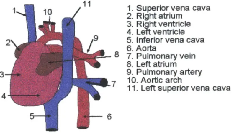
8.0 Anatomy of the Mouse Heart ...

... 59

9.0 Electro physiology ...

61

10.0 Experimental Setup & Procedures ...

...

68

Results/ Discussion

11.0 Best dose of Gd-BSA to use ...

12.0 Optimal parameters for IR turboFLASH (GEFI IR) ...

78

13.0 Optimal parameters for RARE IR ...

85

14.0 Comparison between histology and final infarct images ... 91

15.0 Overall Discussion of Study / Future Studies...

102

Reference

16.0 Bibliography ...

....

106

1.0 Acknowledgements

I want to thank all those who contributed in teaching me about magnetic resonance imaging and

encouraging me during the process of my study. I came to the lab without any prior experience or knowledge of MRI, only the desire to learn and to be able to contribute to the field of cardiac study. I left with a wealth of information on MRI, a new perspective on science, and a reinforced commitment to the study of medical science.

In particular I owe a great debt of gratitude to my supervisor Deborah Burstein. She had the insight to keep a hawk's eye on me during my initial weeks with the lab and then to offer me the space to grow and explore on my own once I was comfortable. She was also pivotal in teaching me not just MRI, but healthy problem-solving techniques in science, a skill which I know shall prove invaluable no matter which field I pursue.

My parents and brother were a spring of abundant support. Through the many hours of late night

experiments and writing, they were always on the phone to offer me a word of encouragement. Both my friends and lab mates deserve my hearty thanks too for their kindness during the moments of frustration every research student must encounter. In particular Jeeva Munasinghe, the lab manager, was invaluable in my education of MRI. Despite his workload he always took the time to explain obscure concepts to me and give me a hand when the hardware systems would

fail.

To all these people I offer my heart-felt thanks.

2.0 Introduction

Motivation:

The need to detect underperfused myocardial tissue is motivated by two reasons mainly:

1) Reparative efforts: Many therapeutic decisions (such as revascularization) depend on the extent of damage in the myocardium. Furthermore infarct detection can help scientists gauge the effectiveness of various pharmacological interventions in preventing and reversing myocardial necrosis.

2) Understanding mechanisms underlying the heart's natural recovery: With advances in our ability to modify the genetics of mammals, cardiologists are now better able to

understand the effect of different genes on cardiovascular function and disease. Typically the gene being studied is either ablated ("knocked out") or modified and the development of the resulting phenotype studied over the course of its lifetime. This technique enables scientists not only to model and understand a particular heart disease but to also

scrutinize the biochemical mechanisms underlying the heart's recovery from this disease or a heart attack for that matter. [Ruff, 1998 #20]

While analytical tools for in-vivo cardiac measurements have evolved extensively for large mammals such as humans and pigs, the techniques remain less developed for smaller animals such as rats and mice; this is not due because smaller animals are unpopular. In fact murine models are heavily used in modeling cardiac conditions because of their technical and economic advantages in genetics studies. The limiting factor in developing tools for smaller animals lies in the technical difficulties posed by their size (heart size 5-8mm) and rapid heart rates (ten times that of humans, meaning 600-700 bpm).

Because MRI offers the flexibility in choosing the imaging plane, multi-slice acquisition, and most importantly high spatial and temporal resolution, it stands out as a powerful imaging tool for evaluation of the myocardium in mice. [James, 1998 #33]

Goal of Study

Among the physiologic parameters that scientists aim to quantify in order to determine the status of the myocardium is perfusion. Perfusion is defined as milliliters of arterial blood entering I Og of tissue per minute.

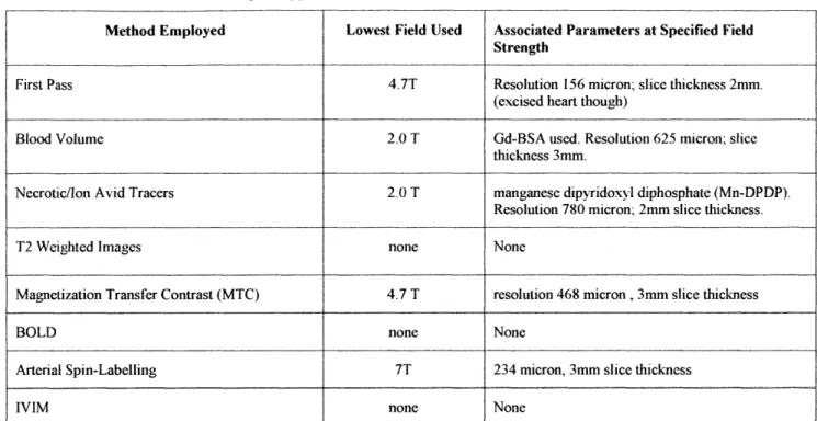
Infarcted and ischemic tissue both have low perfusion numbers relative to healthy myocardium. The goal of this study is to be able to detect perfusion defects in murine myocardium with MRI. The main focus is on evaluating the effectiveness of various pulse sequences and parameters in imaging perfusion defects. In order to improve differentiation between perfusion defects and healthy myocardium, the hearts were enhanced with the contrast agent, gadolinium-DTPA bound to bovine serum albumin (Gd-BSA). We opted to use a blood volume technique as opposed to other perfusion imaging methods such as first pass, ASL, magnetic transfer, BOLD or IVIM because of the better signal to noise ratio at a 2.OT field as well as the steady-state nature of this imaging technique. Gd-BSA was chosen specifically because of its intravascular nature and its growing popularity as a blood contrast agent in recent times.

3.0 Basics of MRI Theory

Skeleton

3.0 Introduction

3.1 The Semi-classical Model

3.2 Understanding TI, T2, and T2* and How to Measure Each 3.3 2-D Image Acquisition

3.4 Averaging, Spatial Resolution, Matrix Size, and FOV

3.0 Introduction

This section introduces the basic concepts of Magnetic Resonance Imaging. Emphasis is placed on the concepts most relevant to the topic of this thesis. For a more in-depth explanation of the concepts, the reader is referred to the texts cited in the bibliography. The theory underlying MR imaging can be explained in terms of a quantum model, however for the sake of simplicity, most texts choose to explain MR behavior via a semi-classical model. In this section we shall rely mainly on the semi-classical model, touching only briefly on some quantumn concepts.

3.1 The Semi-classical Model Equilibrium State

Magnetic resonance imaging relies on the inherent magnetic properties at the nuclear level, specifically only nuclei with an odd number of protons or neutrons. Among the atomic isotopes that can be imaged with magnetic resonance techniques are Hydrogen-1, Carbon-13, Fluorine-19,

and Phosphorous-3 1. In imaging anatomical structures hydrogen-I is often the atomic nuclei of choice because of its sensitivity and abundance in biological samples. Hydrogen nuclei have a spin number equal to /2. The spin number is a simple way to describe the number of energy states and geometry of a nucleus; in this case hydrogen nuclei have two energy states.

Under normal conditions, a population of spins are randomly oriented and split relatively evenly between the two energy states. However when subjected to a magnetic field B0, the atoms act in coherence. A spin % nucleus (1H nucleus) precesses around the B in two possible orientations

(see Fig 3. 1 a) where each orientation is associated with an energy state. The motion is similar to that of a spinning top and has an angular momentum, A.

(b)

(a)

Figure 3.1 : Spinning top model (a) and M, (b)

Given that the nucleus has a charge, it also has magnetic moment p, which can be related to the angular moment (A) by a constant known as the gyromagnetic ratio, y (Eq 3.1). The

gyromagnetic constant for Hydrogen-I is 4258 Hz/G. The torque equation basically states that the angular momentum is the result of the torque exercised by BO on the magnetic moment (Eq 3.2):

=yA (Eq 3.1)

dA = p x B (Eq 3.2) dt

The magnetic moment precesses about the axis of the B0 field at wo, called the Larmour frequency, which can be derived from Eq 3.1 and Eq 3.2

w. = yB0 (Eq 3.3)

As mentioned earlier, in a population of atoms influenced by B0, each hydrogen spin aligns itself in one of two possible orientations depending on its energy level. The exact proportion of spins

oriented parallel and anti-parallel to B0 is a function of the thermal energy in the system and can be described by the Boltzmann distribution. At equilibrium the distribution of spins is:

Nu = e -(yhBo/kT)

N, (Eq 3.4)

where N, and N, correspond to respectively the spin population in the upper and lower energy levels, k represents the Boltzman constant and T is the sample temperature in Kelvin. At room temperatures in a magnetic field of 2.OT, the ratio of spins in each state is close to unity with the small excess of spins being in the lower energy level NI; though the population difference is small, it is still sufficient to be detectable. Conventionally we represent the equilibrium bulk magnetization MO in an external field as a vector in parallel with B" (see Fig 3.1 b). [Horowitz, 1994 #53]

Relaxation

It is necessary to perturb MO away from B0 in order to measure MO independently. This is achieved by sending in an RF pulse with frequency close to w, that flips M0 90 degrees into the x-y plane. Mo then precesses in this plane such that we can measure the magnetization by placing a surface coil (receiver coil) as shown in Fig 3.2. This makes use of Faraday's law to generate an electric signal known as the free induction decay signal (FID), from the rotating magnetization.

Receiver

MO

As soon as the RF pulse ends, three things will happen: 1) M, rotates about B,, and generates an FID 2) the transversal component of MO will decay and 3) the longitudinal component of the magnetization will recover to its original strength. Transversal relaxation is known as spin-spin relaxation and results from the spins interacting in such a way that they de-phase. The time for the transversal component to decay is known as T2, hence the term T2 relaxation. The transversal

component can also dephase due to inhomogenities in the Bo field, which results in an even faster relaxation time described by the constant T2*. In order to acquire an FID it is necessary to refocus de-phased spins via a 180-degree pulse, known as a spin echo. Typically in an experiment

one may see a 90 degree RF pulse followed by a 180-degree pulse before which an echo can be acquired.

Longitudinal relaxation is known as spin-lattice relaxation because spins exchange energy with their environment as they return to their equilibrium state. The time constant associated with this process is T1. The specific time kinetics of both TI and T2 relaxation can be described by the Bloch equations. When the magnetization is tilted into the xy-plane, the return to equilibrium of the magnetization along the z-axis is:

M,(t) = M, [1-e""")] (Eq 3.5)

In MRI experiments, signals are repeatedly generated at a constant repetition time (TR), thus establishing a steady state magnetization described by M\, = M I -e(-TRTI

1.

the magnetization as an echo (while M in the transverse plane), then we have to take into account T2 effects and the time to the echo, TE. Eq 3.5 then takes on the form:

MY M[1-e )] e(- 'E (Eq 3.6)

3.2 Ti-Weighted Images, T2-Weighted Images, And Spin Density Images

Within any sample being imaged, different components ex. tissue vs blood, have different relaxation constants and spin densities. By manipulating the MR pulse sequences, it is possible to make use of a sample's inherent MR properties to create contrast between the components within the sample being imaged. For instance in TI-weighted images, the intensity contrast between any two tissues in an image is due mainly to the TI relaxation properties of the tissues. T2-weighted images are weighted on T2 properties and spin density images are weighted on which substances have more hydrogen nuclei.

To produce a TI weighted image, we use a short TE to eliminate the effect of T2 and a short TR in order not to eliminate the effect of Ti. The topic of how to generate Ti -weighted images will be covered in more depth later since our study relies heavily on this method. With respect to T2-weighted images, these can be generated by using a long TR to eliminate the effect of TI and a long TE in order not to eliminate the effect of T2. The third kind of image, a balanced or spin density image, uses a long TR and a short TE thus eliminating TI and T2 effects.

Methods to Measure Ti

Two popular methods exist for measuring the TI of a biological sample, the saturation recovery method and inversion recovery method. The main objective behind TI measurements is to monitor the growth of M,; this can be done with from the case where M, begins at some value other than M, or -M (saturation recovery) or the case where Mz begins at -M (inversion recovery). Methods exist likewise to measure T2, however they are not covered here since they were not implemented in our study.

The saturation recovery technique involves flipping M,, into the transversal plane with a 90 degree pulse, then measuring the progressive re-growth of the longitudinal magnetization from 0 to M,. Measurements are made by successive steady-state experiments in which TR is varied. The measured magnetization is fitted to the Bloch equation as shown by Eq 1.6 in order to get TI.

Inversion Recovery

With the inversion recovery method of measuring TI, the magnetization is initially flipped by

180 degrees such that M, = -M. Once perturbed M, will recover exponentially to reach

equilibrium, M. The exponential recovery of the magnetization is expressed by the following Bloch equation:

Mz = M( - 2 e") (Eq 3.7)

At various times during this recovery process, Mz can be measured by flipping the magnetization into the x-y plane and measuring it. The time between the 180-degree pulse and time at which the M, is flipped into the transversal plane is referred to as the inversion time, TI. The inversion recovery method requires several acquisitions over which TI is varied. The advantage over the

saturation recovery technique is the increased dynamic range of magnetization that is available because the magnetization varies from - M, to M0 (in contrast to 0 to Mo). However the

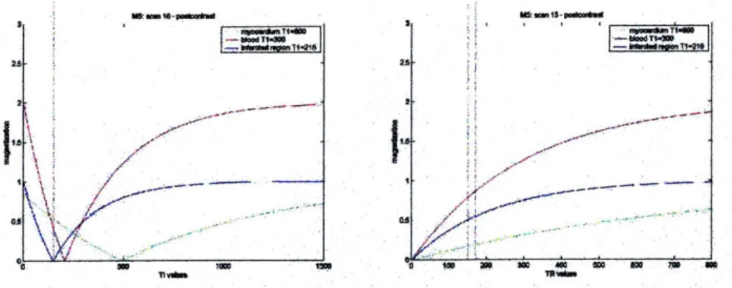
disadvantage of the technique is that TR must be close to 5*TI in order to allow full relaxation between experiments. Fig 3.3 shows a comparison of the data curves generated by the inversion recovery method vs. saturation recovery method.

Fig 3.3 : Inversion Recovery curves (Left), Saturation Recovery Curves (Right).

3.3 Two Dhmensional Imaging

The subject of translating a FID to a 2 dimensional image is intricate and is best understood by breaking the discussion down into 2 main sections: K-space construction and the general format of pulse sequences. Our discussion introduces the concepts of 2-D imaging from a mathematical perspective and in a very brief manner; the reader is once again referred to the bibliography for a more in-depth discussion.

K-Space & Gradients

With some basic math we can relate the spin density of a sample to the signal. We define the following variables for our discussion:

p(r) = local spin density as a function of location r

dV = volume element

w(r)= frequency of precession as a function of location r S(t)= total signal from sample as a function of time

Ignoring constants of proportionality and relying on a simple spin-density image, we know

If we can manipulate the frequency w(r) in such a way that it encodes spatial location, then the

total signal S becomes a function of both space and time; this idea is achieved by using magnetic field gradients. Instead of having one homogeneous external field B0, the field has a gradation such that B = B0 + Ge r, where G describes the slope of the gradient. We know w= yB (Eq 3.3), therefore

w(r)= yB = y(Bo + G * r) (Eq. 3.9)

Note that r represents the x, y, and z directions, and thus G can have a unique value in each of the

3 directions. Now that we have an FID that contains spatial information about the sample, the

next goal is to process the signal to construct an image.

The total on-resonance signal S(t) = p(r)e "r dr

V

We define variable k = yGt/2n, so we can re-write the signal S as S(k) = p(r)e i2nk.rt dr

A close inspection of the expression for S(k) shows that it is the inverse Fourier transform of the

spin density p(r). In other words by taking the Fourier transform of the total signal we can get p(r) which allows us to construct our two dimensional image. Note that the raw signal S(k) as

represented in a two dimensional matrix is referred to as k-space; it is the inverse Fourier transform of the final image. [Callaghan, 1993 #9]

General Format of Pulse Sequences

Gradients are necessary to spatially encode the frequencies in an FID. How the gradients are arranged in a pulse sequence though is another topic. In an x-y-z coordinate system, 3 gradients are necessary in MR imaging. The first gradient is referred to as the slice excitation gradient; it defines the slice which will be imaged. The other two gradients are the "frequency encoding" and "phase encoding" gradients. They define the two directions (e.g. x and y directions) within the

slice to be imaged. Figure 3.4 lists the behavior of the 3 gradients with respect to the pulse sequence (here we show a simple spin-echo sequence).

PHASE() ()()())(0 -(I) h, I It 6 4.,;) ( )r d 7-4.3) 14 1.3) 1.5 1.3 SLICE (0 | 1()()(") It3 -1.4) 01 1. 11 In 9 B sinc3 since

TIeMt S th4 d4 gdu e4 t 12fru 2 .4 1bt dr l de it 4 po 4 12 seltion 4 1.1 12gr ad and4 1.1 12u 2.5u 2t5

L( MPS 3 1-11.4 2 12111 d14 p1 d14 111.4 (it d4 -1.6 12IN 2 1211n 14 2.4 1211u 12 (14 5.1 1211n d4 2.4 12 ou d! d14 vi. 2.511

lo to echo l imres NAECHOES j -lo to slice times N,4]WCES ;I

lo to start times NA -1

-oto statrf

Fig 3.4 - Pulse sequence of a spin echo sequence

Note that the first gradient to be turned on is the slice selection gradient and it occurs during the

90-degree pulse. This ensures that the RF pulse excites only those spins within the slice of

interest, and any signal we see in the x-y plane is from this slice. To understand this concept better, imagine we wish to excite a slice of thickness r centered at zo,. The RF pulse is designed to

have yG zo as the center frequency and a bandwidth of yG,'r. When the RF pulse is turned off, the

spins have de-phased relative to one another and must be rewound prior to measuring the signal.

This is accomplished by reversing the polarity of the slice selective gradient. The

frequency-encoding gradient is applied only when the signal is measured; and the phase frequency-encoding gradient is applied briefly between the time the RF pulse is terminated and the signal is measured. The

frequency gradient and slice select gradient do not vary during an acquisition. On the other hand, the phase encoding gradient varies during the acquisition by increasing steadily with each phase shift repetition.

RF Pulses

RF pulses can be defined by their shape, amplitude, and pulse length. By varying these features one can manipulate slice excitation. It is important to note that the RF pulse is actually generated

by a B, field which lies perpendicular to B. The flip angle induced by pulse is related to the B1 excitation profile by:

0= 7 BI(t)dt (Eq 3. 11)

This means that if a 6-millisecond pulse that was used to achieve a 90-degree excitation is scaled to last only 3-milliseconds, then the amplitude would have to be twice as much to maintain the same excitation. Generating the correct flip angle is one aspect of an RF pulse; the second aspect is exciting the correct slice.

RF pulses can be described as "hard" or "soft" pulses. Hard pulses excite the full sample whereas soft pulses excite only a portion or slice of the sample. A hard pulse is shaped as a block or square wave. The frequency representation or Fourier transform of a block wave is a sinc wave; thus we see that a hard pulse gives energy to all frequencies with the majority of energy centered around one frequency, w,. Typically there is no slice selective gradient on during a hard pulse, therefore all the spins in the sample are centered around one frequency. In the case of soft pulses the slice selective gradient is turned on to allow for spatial selectivity. The common RF pulse

shapes used for soft pulses are Gaussian or sinc pulses. In the time domain, the sine envelope has its first zero-crossing at t = 1/(Bandwidth). Thus the wider the bandwidth, the narrower the sinc

envelope. A sine pulse in the time domain generates a block pulse in the frequency domain; thus in theory all the targeted frequencies are uniformly excited. The profile of a Gaussian wave in the

time domain is a Gaussian in the frequency domain. A property of Fourier transforms is that the shorter length of the wave in the time domain, the longer the length in the frequency domain; hence a shorter Gaussian pulse excites a wider bandwidth. [Finn, 1999 #54]

3.4 Spatial Resolution, Averaging, Matrix Size and Field of View Field of View

The field of view, FOV, is determined by the phase-encoding and frequency-encoding gradients.

Remember the slice select gradient only chooses the slice, while the other two gradients frame the slice. In order to get a smaller FOV the gradients are made steeper, a state which carried to an extreme could stress the gradient set. The FOV as related to the gradient strength is expressed by the following equation (for phase-encoding gradient)

FOV= 2ni (Eq 3.10)

XGrt

where t is the time in seconds for a phase encode.

Matrix Size

The matrix size defines the number of pixels that create the final image. The size is important in determining the spatial resolution of an image as well as the acquisition time for an image. For instance for a given FOV, going from a 64 x 64 matrix to a 128 x 128 matrix doubles our spatial resolution but at the same time doubles our acquisition time. Decisions on the matrix size depend on the priorities of an experiment.

Spatial Resolution

Spatial resolution is calculated as the FOV divided by the matrix size; it is in short the pixel size of the final image. While greater spatial resolution is better, this also implies that there are fewer

spins within each voxel and therefore less signal, leading to what is termed low signal-to-noise ratio (SNR). For instance if we reduce the pixel dimensions by half, the SNR drops by a factor of 4, and in order to attain the same SNR, it is necessary to acquire 16 times more scans (i.e. average

16 times). The other extreme of too high a resolhtion is too low a resolution which leads to many

details of the image being lost (known as volume averaging).

Averaging

Averaging refers to the number of times that the data is obtained. What the MR scanner does is to utilize multiple RF pulses and signal measurements before going on to the next phase encoding step. Images obtained through the use of multiple excitations have a greater signal to noise ratio and usually appear "clearer" than those obtained with only one excitation. However, this comes at a cost; the time required for acquisition becomes multiplied by the number of excitations chosen; in other words, averaging twice would mean that acquisition time is doubled. The SNR however is not doubled- it increases by vr2 since signal doubles but random noise increases by

f.

4. Sequences Used in Cardiac Imaging

Skeleton

4.0 Introduction - Triggering a Sequence and Segmentation 4.1 TurboFLASH/GEFI

4.2 RARE 4.3 EPI

4.4 Flow Effects

Selective vs. non-selective inversion pulses Gradient vs. Spin Echo

4.5 CINE loops

4.0 Cardiac Imaging : Triggering and Segmentation

Perhaps the most significant difference between imaging the heart and imaging another organ is the fact that the heart is a moving object. If during the acquisition of phase encode lines, the heart is each time in a different spatial location, then motion artifact is introduced into the image (seen as smearing or banding of the signal in the phase encode direction). One option to overcome this hurdle is to acquire each phase encode at the same point in the cardiac cycle, when the heart is relatively in the same position. In other words if 64 phase encodes are required, each phase encode would be acquired a given time t after the R wave of the EKG, thus requiring a total of 64 heart beats to create a full image. A variation on this method is to capture several phase encodes at a relatively stationary point in the cardiac cycle, termed segmented k-space data acquisition. For instance if an image echo took 5ms and the isovolumetric contraction period of a heart lasted

25 ms, one could get 4 phase encodes in one heart beat; in the case of our previous example, instead of requiring 64 heart beats to create an image, we would only need 16. The acquisiton time for a segmented sequence can be generalized as:

Typically triggering is tied to the

Q

contractions. In some experiments gating is tied to both the ECG and respiration in order to minimize motion artifact further. For small rodents such as mice and rats, some studies consider this unneceassary since the ratio of respiration to heart rate is 1:10 [Ruff, 2000 #2 1].

The decision as to how many phase encode lines one can capture per cardiac cycle depends on several considerations. First we must know how long the stationary period of the heart lasts. As shown in the section on Cardiac Cycle, the diastolic period of the heart is relatively stable and lasts atleast 100ms in CB57 L/6 mice. Even though we may have a sequence that could acquire 20 phase encodes in this window of time, T2 decay can sometimes render this attempt useless (for instance in RARE). Another consideration is also the sequence itself, whether it has the capability to do multiple phase-encodes within one cardiac-cycle. These issues will be presented in the context of a number of different fast imaging sequences in the sections below. Additionally flow

effects will be discussed. Among the popular fast sequences that will be covered are turboFLASH, RARE, and EPI.

4.1 TurboFLASH

TurboFLASH is known by several other names such as gradient echo fast imaging (GEFI), SPGR (spoiled GRASS), and RF-FAST (RF spoiled Fourier acquired steady state). The technique is not as fast as echo-planar imaging (EPI), however it does not require the specialized hardware associated with EPI. The essence of the sequence is that it employs a short TR (on the order of

2-10 ms) followed by a pulse with flip angle a and then a gradient echo. Because the TR is too

short to allow full relaxation of the longitudinal magnetization, it does not benefit the SNR to have a flip angle of 90 degrees after each TR. Instead the flip angle is optimized to the Ernst

angle, a. The relationship between the flip angle a, TR, and TI of the samriple is shown below by Equation 4.1.

a cos -(e "") (Eq 4.1)

Furthermore the relative signal can be estimated as

-- T I T i

1-e--TRITI

SGR =M e TE '2 * (Eq 4.2)

With human hearts, turboFLASH has enabled researchers to complete acquisition of a full image in one cardiac cycle. One of the earliest studies to utilize a turboFLASH sequence to image the heart was conducted by Frahm et al. At a field strength of 2.OT, the TR was made as short as 4.8ms and a = 10 0. The result were heart images that could be acquired in 4.8ms * 64 phase

encodes = 307 ms, which meant one could afford a time resolution of one image per heart beat. In rodent imaging, the heart rates are often so fast that it is sometimes hard to acquire one image per heart beat. The alternative is to use a segmented turboFLASH sequence [Frahm, 1990 #30].

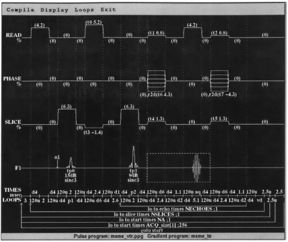
An inversion recovery turboFLASH sequence is a small variation in the normal turboFLASH sequence in that it is preceeded by a 180 0 inversion pulse. Figure 4.1 shows a diagram of the

Figure 4.1 - Pulse sequence for a IR turboFLASH pulse program.

4.2 RARE & Inversion Recovery RARE

RARE imaging which stands for Rapid Acquisition with Relaxation Enhancement, is also known

by other names such as turbo spin echo (TSE) or fast spin-echo (FSE). Compared with

conventional spin echo imaging, the most important feature of RARE imaging is that several

phase-encoding lines are collected with multiple echos. The pulse sequence is shown below in

Fig 4.2. As illustrated in the figure, the RF pulse scheme includes an excitation RF pulse,

typically using a flip angle of 90 degrees, followed by several refocusing RF pulses. One can also

note that the appropriate phase-encoding gradient for each echo is applied just before the data-sampling period. Subsequently just after data data-sampling is complete, a phase-encoding gradient for each echo with equal amplitude but opposite polarity is applied to rewind the effect of the first gradient. In this way, all the echoes will be encoded equivalently. RARE imaging posses many of

the characteristics of conventional spine echo imaging but has the important advantage of much

shorter acquisition times, which can be traded for increased resolution. RARE sequences also

provide more T2 weighting as a result of the increased TE time.

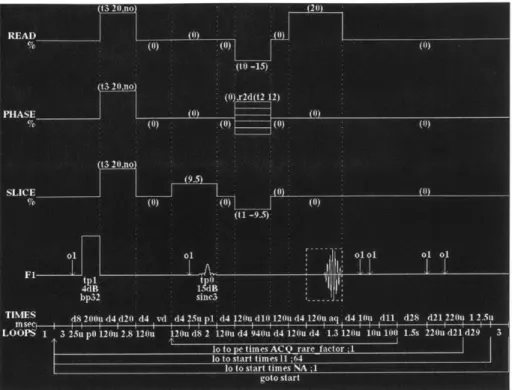
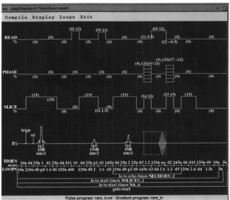
Figure 4.2 - Pulse sequence for RARE IR

Inversion Recovery RARE only differs from the normal RARE sequence by having a 180 degree

inversion pulse at the start. Like with IR turboFLASH, this adds greater TI-weighting to the image.

4.3 EPI/ Multi-echo spoiled gradient-echo imaging

Because EPI was not implemented in this study, the sequence is discussed only briefly here. Single-shot EPI was first introduced by Peter Mansfield in 1977. In his work, Mansfield

described the collection of the entire k-space dataset by alternating the gradient set during a single echo after 90 degree-180 degree (spin-echo) excitation. This allows for a very rapid collection of

datasets with very high sequence efficiency. Gradient-echo EPI is an alternative form of EPI that plays the readout train immediately after slice selection, increasing sequence efficiency and reducing acquisition times. EPI has very low imaging times; sometimes entire images are taken in 40-120 ms. However it is prone to substantial image artifacts from field inhomogenities, and susceptibility interfaces and fat [Reeder, 2000 #44].

4.4 Flow Effects

Selective vs. Non-selective Inversion Pulse

Inversion recovery serves to provide more TI-weighting than a regular gradient-echo or spin-echo sequence. Note in Figure 4.1 of the turboFLASH sequence, that the the 180-degree pulse is nonselective while the a -degree pulse is selective. The reason for this difference lies in

manipulating the signal of the blood. If both pulses were selective (i.e. the spins in only a given slice were excited) then by the time the a -degree pulse were applied to the sample, some of the spins in the blood affected by the inversion pulse would have flown out of the slice and the a

-degree pulse would affect fresh fully-relaxed blood entering the slice. The result is that blood may appear brighter in an image. The assumption made here is that the time between the 180-degree pulse and a -degree pulse (inversion time, TI) is long enough to allow non-inverted blood to flow

into the slice.

Blood in the macrovascular structures such as the ventricles and atria tends to flow rapidly during the cardiac cycle, thus blood almost always appears bright in these structures. What about

microvascular structures? Myocardial perfusion rates in mice have been shown to be around 0.06ml/s/g, thus if we have a TI of 500ms, we lose 50% of the inverted blood spins in a slice if we use two selective pulses.

What if were to use a non-selective inversion pulse followed by a selective a -degree pulse as suggested in Figure 4.1? Then all the blood in the sample is excited, so that the a -degree pulse sees no difference in the blood it affects within a given slice. The signal enhancement previously seen in both myocardium and macrovascular structures due to blood flow is omitted with this technique [Pettigrew, 1999 #31].

Gradient Echo vs. Spin Echo

Another important consideration is whether flow effects manifest themselves over the time of TE. Because gradient echos provide short TEs (on the order of 4-5ms), we see relatively little flow effect in the myocardium due to perfusion. The same applies to macrovascular structures if the heart is at a quiet point in its cardiac cycle. If the heart however is in peak systole and blood is being ejected during the time of the gradient echo, there will be some signal loss in the ventricles,

seen often times as dark spots in the ventricle.

Pulse sequences make use of either a gradient echo or spin echo in order to acquire the signal. Each type of echo emphasizes different aspects of a cardiac image. In the case of a spin echo, the signal is significantly less sensitive to field inhomogenities (i.e. T2* effects). Gradient echoes though sensitive to T2* decay usually have short echo times, which minimize the effects of short

T2* commonly observed in the heart and minimize the effect of motion.

4.5 CINE imaging

In cine imaging snapshots of a particular slice of the heart are taken throughout the cardiac cycle such that they can be strung together to create a picture of the muscle dynamics within a slice. To make a "cine loop", images of a slice are taken at differing times in the cycle by varying the sequence's trigger point relative to the R wave. To get a sense of the acquisition times required to make a cine movie, assume we use a single gradient-echo sequence with TR equal to the RR interval. If we wish to fill a square matrix of dimension N and gather P number of images of the cardiac cycle, then the acquisition time would be

Acquisition time = N * P * (RR interval)

Typically the interest is to create a cine movie of several slices of the heart rather than one. We can excite a single slice, acquire a signal from it, and then wait TR for it to recover before repeating the process. If we have S slices, the acquisition time becomes

Acquisition time = S * N * P * (RR interval)

A more efficient method for multi-slice CINE imaging is to interleave the acquisition. During the

TR for one slice, it is possible to excite another slice or multiple slices such that the acquisition points for all the slices will be interspersed throughout the cardiac cycle. This method can

sometimes drop the acquisition time to N * P * (RR interval). One important consideration is that adjacent slices should not be imaged consecutively since excitation of one slice may bleed into the other (due to imprecise slice excitation by RF pulse).

5.

Methods in Myocardial Perfusion Analysis

Skeleton

5.0 Introduction -what is perfusion? What are perfusion-defects?

5.1 Where we currently are in perfusion defect detection in large mammals such as humans. A

break down of the various methods.

Exogenous Methods

5.1.1 First Pass -- Theory. Experimental needs. Qualitative & quantitative studies.

5.1.2 Blood Volume - Theory & Experimental concerns. Data. Contrast Agents.

5.1.3 Other Recent Exogenous Methods - Necrotic-avid tracers & ion contrast media

Endogenous Methods

5.2.1 T2 weighted images - brief theory.

5.2.2 MTC - magnetization transfer contrast- theory & most pertinent study so far. 5.2.3 BOLD - theory and explanation of myocardial studies.

5.2.4 ASL & FAIR -theory

5.2.5 Intravoxel Incoherent Method (IVIM) - brief description. No theory this time.

5.3 Where we are with smaller animals such as rats and mice. A breakdown of methods used in

small mammals.

5.0 Introduction

Since scientists aim to investigate the viability and function of a tissue, being able to study the perfusion level in myocardial tissue is of great interest to those in cardiology. Perfusion is defined as milliliters of arterial blood entering 1 OOg of tissue per minute and is in essence a process which controls the delivery of nutrients to tissue. Perfusion, f, can be calculated as :

f= F/V where F arterial blood rate (ml/min) (Eq 5.1) V tissue volume (ml).

Often times the strict meaning of perfusion has been relaxed so that in some literature, the term refers to the degree of normal or abnormal vasculature in a tissue. Perfusion has sometimes been confused also for referring to blood-tissue exchange. An analogy is helpful in steering clear from confusion on this point. Imagine a radiator in a room. Perfusion is similar to measuring the water flow through the radiator. It is not to be confused with the amount of heat transferred from the radiator to the surrounding enviromnent nor the number of pipes- though these parameters are related to perfusion [Pettigrew, 1999 #31].

This section covers the current techniques implemented to detect perfusion defects in the

myocardium. By perfusion defects we mean regions of the myocardium where the perfusion level is lower than normal/healthy myocardium for the particular species under investigation; note this definition encompasses ischemic and infarcted myocardium. The summary of current MR techniques is broken down into those utilized for larger manunals such as humans and pigs and those that have been applied to smaller animals such as rats and mice. This separation is

necessary since many of the techniques described for large animals are hard to apply to rats/mice at a given field strength due to their smaller heart sizes and faster heart rates.

5.2 Current Perfusion Analysis Methods for Large Mammals

Perfusion imaging techniques can be broken down into two main categories: exogenous contrast techniques and endogenous contrast techniques. In exogenous contrast techniques a relaxivity agent is injected into the region of interest and the region then imaged either for tracer time-kinetics or for the tissue's state under steady-state conditions to ascertain useful physiologic information. A relaxivity agent is a drug that reduces the relaxation time (TI and T2) of water protons in the sample being imaged. Typical relaxivity agents used are paramagnetic chelates, most notably gadolinium-DTPA (Gd-DTPA). Gd-DTPA decreases both TI and T2 rates but is

known as a TI agent because rate constant changes based on a percentage are much greater for TI compared to T2. Among the most popular imaging methods for measuring perfusion with exogenous agents are first-pass and blood volume methods, which are explained in detail in the sections below. In first pass studies a bolus of contrast agent is injected and the time kinetics of the contrast agent are studied in the tissue to determine perfusion. In blood volume studies, an intravascular contrast agent is injected into the body and allowed to reach steady-state. Because an intravascular agent does not leave the vascular space, one can equate blood volume to the volume in which the agent is restricted. Though blood volume is not a direct parameter to detecting perfusion defects, it is strongly correlated to perfusion levels [Pottumarthi, 1995 #28].

Endogenous contrast techniques make use of the tissue or blood's inherent properties to gather physiologic information. There are a number of such techniques. One common technique known as BOLD uses the blood as a contrast agent. Oxygenated blood is diamagnetic and becomes paramagnetic when deoxygenated. A boundary interfacing the paramagnetic venous blood and tissue generates susceptibility effects that can seen in an MR image. Therefore an increase in regional blood flow means blood is better oxygenated which in turn will be reflected in the MR scan. Another endogenous contrast technique is the intravoxel incoherent motion method (IVIM). Based on its sensitivity to diffusion effects, IVIM assumes that the motion in capillaries is similar to that of random diffusional motion and attempts to detect this. The method proves to be

complicated and indirect in its measurement of perfusion [James, 1998 #33]. A third approach uses magnetically tagged endogenous water (sometimes referred to as FAIR, Flow-sensitive Alternating Inversion Recovery, or ASL, Arterial Spin Labelling). In this method a flow-sensitive image is subtracted from a flow insensitive image [Andersen, 2000 #55].

Below is a more indepth look at the exogenous and endogenous contrast techniques already touched upon plus some additional techniques that have been developed in the last two years.

Exogenous Techniques

5.1.1 Bolus Tracking/First Pass

Over 500 studies have been conducted on patients utilizing MR first pass techniques. The basic

technique involves injecting a contrast agent as a bolus into the patient and then observing the

time kinetics of the chemical in the tissue. Regional myocardium with perfusion defects will have

different enhancement patterns over time as compared to normal myocardium. An example can

be seen in Figure 5.1 where the abnormal region shows early hypoenhancement after the patient

is injected with Gd-DTPA.

Figure 5.1- First-pass pictures of myocardium showing early hypoenhancement (ischemic region).

Theory

The theory behind MR first pass imaging is based on the earlier indicator-dilution methods

employed in nuclear medicine for studying perfusion. When a nondiffusible contrast agent is

injected into the bloodstream in the form of a bolus, the movement of blood through an organ can

be studied by observing the signal intensity changes over time induced by the blood flow.

Changes are due in part to two reasons- relaxivity effects and susceptibilty effects. The presence

of a contrast agent decreases the TI and T2 of blood and tissue. The high susceptibility of the

contrast agent also produces steep, localized magnetic fields that are reflected in a decrease of

-T2*. Whether relaxivity or susceptibility effects dominate in an image depends on the imaging sequence used. [Pettigrew, 1999 #31]

Assuming one adheres to certain experimental criteria to obtain concentration-time curves, the next step is to extract the relevant perfusion information from the data. This can be done using the

central volume principle which states that absolute blood flow (BF) is:

BF = Vd/MTT Equation 5.2

where V, is the volume fraction of the contrast agent in a tissue and MTT is the mean transit time.

V, for a freely diffusible agent is equal to 1 since the chemical diffuses throughout the entire tissue. In the case of an intravascular agent, V is equal to the blood volume Vb (blood volume is defined as the fraction of tissue occupied by blood). MTT, the mean transit time, refers to the average time required for a particle of tracer to pass through the tissue.

V, can be calculated directly from the concentration-time curves as

Vd = ,,_._t

.Caiea(t)dt

MTT can be derived from the concentration time curves by calculating the first moment of the measured concentration-time curve for tissue (this is an estimation of the indicator-dilution methods rather than a precise measure). In the above manner it is possible to apply the central volume principle to the concentration-time curves to get a a rough quantitative measure of perfusion [Pottumarthi, 1995 #28].

Experimental Procedures

Given the theory, it is possible to use a number of different contrast agents and a number of different arterial input functions to measure perfusion. In order to simplify computations and avoid complex deconvolutions, studies often aim to inject a bolus of contrast agent into the patient, thus allowing the arterial input function to be approximated as an impulse. Bolus

injections are not a necessity; a number of studies have shown it is possible to use other arterial input functions, however it does make computations simpler. Another experimental concern is monitoring the time kinetics of the contrast agent as it passes through the organ. Since mean transit times can be fast, first-pass necessitates rapid imaging procedures such as EPI and turboFLASH. For instance in the case of a patient with a heart rate of 50-90 beats/minutes, acquisition should occur every 1 or 2 seconds [Pettigrew, 1999 #31].

Choosing a contrast agent can also impact experimental procedures since it effects the MTTs and volume fraction distribution Vd. In the case that an intravascular agent is used, the volume fraction of the contrast agent Vd reflects the blood volume, a bonus piece of information.

However intravascular agents have a short mean transit time meaning myocardial signal intensity should be sampled quickly in order to get accurate concentration curves. It is possible to conduct first pass studies with non-intravascular agents as well and get slower MTTs. For instance one study attempted to use P760, a gadolinium chelate with slow interstitial diffusion and high relaxivity and found it to work reliably well in pigs [Kroft, 1999 #56]. Some studies have also used non-proton contrast agents such as F'9. Since this species does not appear in the body in

significant quantities, there is little confusion in tracking the diffusion pattern of this contrast agent [Pottumarthi, 1995 #28].

One other issue that needs to be kept in mind is that MRI does not directly measure the contrast agent concentration; the latter is determined by a measure of TI or T2. However calculating

contrast agent concentration from TI and T2 and requires a knowledge of the exhange rate of water betweeen the various tissue compartments [Donahue, 1994 #60]. This is an area under active investigation.

Qualitative & Quantitative Data

Qualitative studies have shown that the enhancement patterns of tissue over time are capable of revealing regions of perfusion defects and furthermore describing the type of defect. For instance patient studies with Gd-DTPA show that in TI weighted first pass images, areas of delayed hyperenhancement compared well with areas of irreversible myocardial damage, known as "fixed defects" [#5, #38]. In general under steady-state conditions, it has been shown that with Gd-DTPA, infarcted areas have a greater signal intensity than normal myocardium.

A number of quantitative studies using first-pass methods have been conducted on humans, pigs,

and other large mammals. Results of the technique have corresponded closely with histological measurements peformed with microspheres, and first pass has become established as a reliable method of ascertaining estimates of myocardial perfusion [Kroft, 1999 #56].

5.1.2 Blood Volume

Blood volume, V,, is defined as the fraction of a tissue volume occupied by blood. While in theory V, for a tissue sample need not correspond to perfusion, experiments have shown a strong correlation between the two parameters; thus ischemic or infarcted areas can often be spotted through blood volume studies [Pottumarthi, 1995 #28]. Like in first pass studies, most blood volume studies involve the use of a contrast agent. The agent is injected into the patient and TI or T2 images are captured after the myocardiumn reaches a steady-state. One notable advantage of blood volume studies over first pass techniques is that the state of the tissue does not need to be

studied over a time course, therefore eliminating the need for fast imaging sequences. Figure

5.2

below displays an example of a blood volume study in which Gd-DTPA was used in an ex vivo

and a T1 image captured. The bright areas

in

the myocardium reflects the infarcted tissue and can

be seen to correlate with TTC staining.

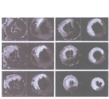
Figure 5.2- Blood volume pictures with Gd-DTPA showing infarcted area as hyperenhanced. MR images on

right and corresponding TTC stains on left.

Theory & Experimental Procedures

This section briefly covers the theory behind computing reginonal blood volume (RBV); for a more detailed understanding refer to the section on "Tissue Models for RBV". As explained in the section on first pass imaging, one can calculate the blood volume of a tissue by using an

intravascular agent and acquiring concentration-time curves. Applying the equation below we can extract from the cocentration curves, the volume distribution fraction of the agent Vd which in

Vd =

tssuetdt

.f

If we allow t to go to infinity, i.e. allow the system to reach steady-state, we can approximate V,

as the concentration of agent in the tissue divided by the concentration of agent in arterial blood. The process of calculating concentration curves from image maps can be cumbersome and so most studies use an related method to measure the blood volume in myocardium. By measuring the Ti of a tissue sample before an intravascular agent is administered and then measuring it again after administration, one can apply the equation below to get an approximation of the regional blood volume:

Vb= I /IP-1I/TI MIA 1/T ipre_ 1/T1,osI

Typically studies inject multiple doses of a contrast agent to get multiple T I maps and thus gather more reliable data on the blood volume levels in myocardium. The use of multiple T I maps also

has another advantage. Equation 2 is a simplification of a more complicated equation which includes the effects of perfusion to get a more accurate estimate of V. In order to use the more precise equation, multiple TI maps are required [Kahler, 1998 #27]. For the purposes of keeping this discussion simple, this equation nor method will be fully explored in this section (please refer to the section on Tissue Models for more details).

Quantitative & Qualitative Data

While quantifying regional blood volume is useful in detecting perfusion defects, it is possible to also rely on qualitative data. Steady-state images after administration of a contrast agent such as

Gd-DTPA have clearly shown that ischemic areas appear darker/brighter than normal

myocardium in TI-weighted images. An example of this behavior can be seen in Figure 5.2. This result is based on the fact that the contrast agent, which shortens TIs, travels via the blood and is able to effect ischemic areas less than normal myocardium due to depressed blood volumes. Studies have been conducted to determine the relationship between qualitative detection of ischemic/infarct detection using blood volume and first-pass methods. This relationship obviously depends in part on the contrast agent used. One study compared the effectiveness of contrast enhanced Gd-DTPA TI-weighted blood volume and MR first-pass imaging for accurately estimating the size of infarcted regions in pigs. Steady state Gd-DTPA TI-weighted images showed that the areas of abnormal signal intensity were larger than the defective areas spotted by first-pass. By comparing the MR results against histology, the conclusion made by the study is that first-pass is effective in detecting infarcted areas while the other technique seems to include the peri-infarct. The peri-infarct area or boreder zone is defined as the area of reversibly injured myocardium adjacent to the core of an infarct [#3, #34].

Contrast Agents

Both extracellular and intravascular agents can be used to study blood volume, however

intravascular agents (blood pool agents) provide better estimates of blood volume. These agents cannot pass the capillary pores because of their molecular weight (usually on the order of 12-150 kDa) and thus stays in the blood for long periods of time unlike extracellular agents which dissipate into the interstitial area. A number of studies have been conducted in the past to verify the effectiveness of different contrast agents in blood volume studies. Among the newest agents to be used are gadolinium chelates such as Gd-BSA and Gd-polysine. While most contrast agents seem best imaged with TI-weighted sequences, there are agents that benefit from T2-weighted images. For instance one study used a ultrasmall superparamagnetic ironoxide (USPIO) preparation known as NC 100150 and found that imaging with a T2-weighted turbo spin echo

sequence gave the reliable indications of differences in myocardial blood volume [Bjerner, 2000 #43].

5.1.3 Other Methods Which Employ an Agent

Researchers have also investigated the use of nectrotic-avid agents such as gadophrin-2 to detect a class of perfusion defects, infarcted/nectrotic tissue, and have met with promising results. Studies suggest that necrosis-avid tracers might even be more precise in defining necrotic areas than agents such as Gd-DTPA, which are said to overestimate infarcted areas by about 10%. The

downside of this agent is that it takes 1-3 hours after administration before imaging can take place. Note that this contrast agent does not fall within the scope of blood volume studies since

agent concentrations in myocardium depend on the amount of necrotic tissue rather than blood in a tissue [Pislaru, 1999 #45].

Similar to necrotic-avid tracer methods are ion contrast media methods such as "Na, twentry-three sodium, MRI. This method is based on the fact that irreversible myocardial injury and

myocyte death are characterized by loss of cellular membrane integrity and of normal electrochemical ion gradients resulting in accumulation of intracelullar sodium and water in necrotic cells. Although it is possible to detect these increases in intracellular sodium by

administering "Na, these agents cannot be used in vivo because of their high toxicity. More recent studies suggest that total sodium may be used as an indictation of ischemia [Gerber BL, Top Magn Reson Imaging #8]. MnDPDP (manganese dipyridoxyl diphosphate), also known as Teslascan, works in a similar way. When administered in a patient, manganese cations are released into the blood stream and quickly absorbed by viable myocardial cells via

voltage-dependent calcium channels and retained. The result is that the uptake of myocardium is high in normal myocardium as compared with infarcted tissue and differing levels of uptake can then be

spotted with Ti-imaging [Bremerich J, 2000 #5]. As with necrotic-avid tracers, ion contrast media are helpful in detecting infarcted regions and not other perfusion-limited areas such as

ischemic regions [Wendland, 1999 #47].

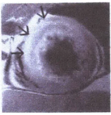
Figure 5.3 - Example of Sodium-23 image where bright area with arrows shows infarcted region.

Endogenous Techniques

5.2.1 T2 Weighted Studies

Studies have reported that TI-weighted imaging without exogenous contrast agents provides little or no information on perfusion defects in myocardium. However the same cannot be said for T2-weighted imaging; infarcted areas have been shown to be detectable with T2-T2-weighted MRI and

show up as hyperintense regions [Lim, 1999 #34]. A study by Lim and Choi showed that the

diagnostic concordance rate between T2-weighted MRI and rest thallium SPECT was 95% when analyzing infarcted areas. The downside of this technique, however, is it does not identify chronic infarcts (i.e. reversible vs irreversible damage) and may overestimate infarct size by including areas at risk. T2-weighted images also often have a low signal-to-noise ratio compared with contrast-enhanced perfusion imaging which provides better-quality images [Gerber BL, Top

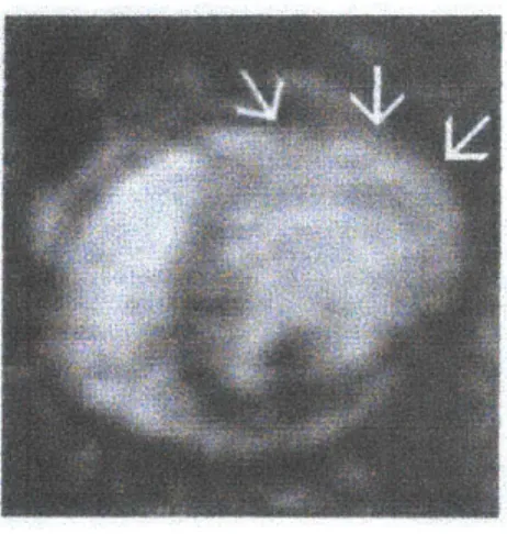
Figure 5.4 - Example of T2 weighted image for detection of ischemic region. Hyperintense area denotes

ischemic region.

5.2.2 Magnetization Transfer Contrast (MTC)

One technique which makes use of the inherent longitudinal magnetization properties of myocardial tissue in order to obviate the need for exogenous contrast agents is Magnetization Transfer Contrast (MTC) imaging. MTC is based on the saturation transfer method being applied to biological tissue. This method relies on magnetization transfer between tissue water with restricted motion, referred to as 'H, and "free" bulk water with unrestricted motion, 1Hf.

Examples of 'H, include water in cellular membranes and macromolecular matrices. By

selectively saturating the 'H, spins, magnetization transfer occurs between 'H, spins and 'Hf spins, and this can be seen in an image as a signal intensity drop in 'Hf. It has been shown that surface hydroxyl and/or amine groups on macromolecular surfaces appear to be necessary for

magnetization transfer. These groups presumably orient water protons in close proximity to macromolecular protons for a time sufficient to allow magnetization transfer to occur. Several

tissues have been shown to have the necessary physiochemical properties for significant

magnetization transfer including myocardium, skeletal muscle, skin, and articular cartilage. Figure 5.5 diagrams the interaction between water spins in an MTC experiment [Scholz, 1993 #50].

40

Mae. cmleeulir M-MA 'Oaundaw9 Ze'4 'QO.A Water Hee'~ H H H H N 0 H H VA"

H~

Figure 5.5 Description of molecular interactions and MT.

Studies have shown that both MT-weighted signal intensity and T18 increase with an increase in

flow rate, thus imaging sequences that weight based on both these parameters can detect relative

differences in perfusion levels. Note Tl

3 is defined as the spin-lattice relaxation time of 'Hf in the

presence of 'H

saturation. An example of some images acquired by this method on an isolated

heart are shown in Figure

5.6.

One can note the efficiency of this method as related to TI imaging

with Gd-DTPA. In this particular study imaging was done with MT preparation pulses followed

by an inversion recovery turboFLASH sequence. The TI for the inversion recovery pulse was

chosen to almost null normal myocardium (not completely), i.e. close to the zero crossing of the

tissue. Since MR images are usually displayed as absolute magnitude values, the Ti-weighted

image intensity taken at a zero-crossing will increase with any change in longitudinal equilibrium

magnetization. Similarly with TI, the absolute magnitude of the TI-weighted signal intensity will

increase for changes in TI values [Prasad, 1993

#5 7].

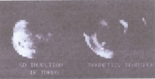
Figure 5.6 -Example of MT images compared with Gd image.

5.2.3 BOLD

BOLD which stands for blood oxygen level dependent contrast, relies on the paramagnetic and diamagnetic properties of blood. Deoxyhemoglobin is a paramagnetic molecule whereas oxyhemoglobin is diamagnetic. The presence of deoxyhemoglobin in a blood vessel causes a

susceptibility difference between the vessel and its surrounding tissue, in other words between

venous blood and tissue. Such susceptibility differences cause dephasing of the MR proton signal, leading to a reduction in the value of T2*. In a T2* weighted imaging experiment, the presence of deoxyhemoglobin in the blood vessels causes a darkening of the image in those voxels containing vessels. Since oxyhemoglobin is diamagnetic and does not produce the same dephasing, changes

in oxygenation of the blood can be observed as the signal changes in T2* weighted images [Miller, 2000 #48]. BOLD has been a technique primarily used in fMRI but some perfusion studies in cardiac imaging have used it as well. Currently no published literature shows that studies have been conducted directly on ischemic tissue detection using BOLD. Instead most of the work has been to prove that a relative change in the perfusion level of overall human myocardium can be detected with this method [Eng, 1991 #49].

42