DETERMINATION OF THREE DIMENSIONAL TRACE ELEMENT DISTRIBUTIONS
BY THE USE OF
MONOCHROMATIC X-RAY MICROBEAMS
by
Paul Boisseau
B.S., Massachusetts Institute of Technology
(1978)
Submitted to the Department of Physics in Partial Fulfillment of the Requirements
for the Degree of
DOCTOR OF PHILOSOPHY
at the
MASSACHUSETTS INSTITUTE OF TECHNOLOGY
January, 1986
@Massachusetts
Institute of Technology 1986Signature of Author Certified by
Signature redacted
Department of Physics January, 1986Signature redacted.
Prof. Lee Grodzins Thesis Supervisor
Signature redacted
Accepted by
MASSACHUSETTS INSTITUTE
OF TECHNIOLOGY
Prof. George F. Koster Chairman, Graduate Committee
M ITLibraries
77 Massachusetts Avenue Cambridge, MA 02139 http://Iibraries.mit.edu/ask
DISCLAIMER NOTICE
The pagination in this thesis reflects how it was delivered to the Institute Archives and Special Collections.
DETERMINATION OF THREE DIMENSIONAL TRACE ELEMENT DISTRIBUTIONS BY THE USE OF
MONOCHROMATIC X-RAY MICROBEAMS
by
Paul Boisseau
Submitted to the Department of Physics
in January 1986, in partial fulfillment of the requirements for the degree of Doctor of Philosophy
Abstract
The technique of x-ray induced x-ray fluorescence analysis has long been used for the determination of trace element concentrations for a wide variety of specimens. The development of high flux density synchrotron beams allows the technique to be extended to provide spatially resolved analysis using x-ray microbeams. X-ray tomo-graphic analysis for the imaging of density variations in the interior of materials has been developed during the past 15 years. In this thesis, the x-ray tomographic tech-nique has been combined with x-ray fluorescence using high flux density monochro-matic synchrotron beams. The result is the first tomographic determination of trace element distributions through the interior of objects. Trace elements are detected by fluorescent excitation of characteristic x-rays along a collimated beam path scanned through the specimen. Tomographic reconstruction techniques are used to determine planar distributions. Estimates are made of sensitivity in the tomographic mode.
Experimental results of the technique are presented.
Thesis Supervisor: Dr. Lee Grodzins Title: Professor of Physics
ACKNOWLEDGEMENTS
Over the last few years, I have been lucky enough to work on a whole range of exciting topics, and my education could not have been more suitable to my interests and abilities. This state of affairs is wholly due to my thesis advisor, Lee Grodzins. Lee always seemed to know when to get me involved in something that was a little beyond my abilities, as well as when to leave me alone. His continous personal and professional concern for me has made all of the difference.
One of my oldest friends at MIT, Bob Ledoux always had the ability to look on the bright side of things, even when there wasn't one. His combination of hard work and easygoing attitude has always been an inspiration, although admittedly it never made much sense to me.
Evita Vulgaris has constantly been a reminder that there are people who are just nothing like me. Her friendship, both in and out of the lab, has been and always will be appreciated.
Bill Nett has been a good friend during all of my student days, and has helped me out in many ways. I will always appreciate his help, even though I have my own car now.
I would like to thank Phil Kesten for his years of friendship and support, as well as for helping out in the Last Days of the Thesis. Next time I will start the thesis a week earlier.
This thesis would have been quite different with no data, and I thank Cullie Sparks and the Oak Ridge synchrotron research group for their support and flexibility.
My first experience with research was with the Scanning Proton Microprobe.
Jean Ryan showed remarkable calmness in the face of a number of near disasters, and allowed me to acquire a great deal of experience over the years.
My first experience with 'real world' research was due to the people at
Eaton/Oxygen. I would like to thank them for the chance to develop the optical tomography project.
for that matter any of the past or present members. I have confidence that the group will always have the peculiar way that made my work at MIT such a pleasure
Finally, I would like to thank the members of my family for the support that they have shown over the years- I hope that the thesis will finally show them just exactly what I have been doing all this time.
TABLE OF CONTENTS Abstract... Acknowledgements ... Table of Contents ... List of Figures ... References ... Chapter I - INTRODUCTION. 3 4 7 8 10 ... 12
Chapter II - TOMOGRAPHIC RECONSTRUCTION... 27
A. Optical M odel ... . 28
B . N oise ... . 38
Chapter III - SYNCHROTRON FLUORESCENCE TOMOGRAPHY. 50 A. Specimen Requirements ... 51
B. Experimental Procedure... 56
C . R esults ... . 65
D. Future Development ... . 65
Chapter IV - Optical Tomography of Ion Beams... 70
Apendix A - NSLS Microprobe Optical System... 89
Apendix B - Ion Induced X-Rays for XRF Analysis... 100
Apendix C - Scanning Rutherford Backscattering Analysis... 115 ... ...
o...
...oo... ... ... ... . ... . ... . ... . ...Fig. 1.1 : Fig. Fig. Fig. Fig. Fig. Fig. Fig. Fig. Fig. Fig. Fig. Fig. Fig. Fig. Fig. Fig. Fig. Fig. Fig. Fig. Fig. 1.2 : 1.3 : 1.4 : 1.5 : 1.6 : 1.7 : 2.1, 2.2 2.3 : 2.4 : 2.5 : 2.6 : 2.7 : 2.8 : 2.9, 2.10: 2.11 3.1 : 3.2: 3.3 : 3.4 : 3.5 : 3.6 : LIST OF FIGURES
Atomic model, showing electron transitions that may follow electron vacancies ...
Fluorescence yields...
K-shell ionization cross-sections...
Comparison of charged particle an photon excitation for characteristic x-ray production ...
Synchrotron radiation Spectra for NSLS...
Photoelectric cross-section for Arsenic...
Synchrotron Tomography...
Optical Tomography...
Algebraic Reconstruction Technique...
Simple Back Projection...
Filtered Back Projection...
Fluorescence spectrum: iron in carbon matrix...
Intrinsic sensitivities, charged particle vs. XRF ...
Tomographic analysis of single point...
Zero-point fluctuation for single point reconstruction...
Statistical noise in low contrast extended specimen... .
Beam parameters, NSLS...
ORNL beam line...
Tomographic scanning stage...
Beam profile at specimen position...
Data collection system... .... ... . Specimen #1, honeybee... 15 16 18 19 21 22 25 30 33 35 36 40 42 43 45 46 53 54 57 58 59 62
Fig. 3.8 : NBS Trace element standard #612... 63
Fig. 3.9 : Accumulated x-ray spectrum, Bee... 64
Fig. 3.10 : Reconstructed image; specimen #1 in Fe... 66
Fig. 3.11 : Reconstructed image; specimen #2 in Fe... 67
Fig. 3.12 : Reconstructed image; specimen #2 in Ti... 68
Fig. 4.1 : Geometry of ion beam scanner... 73
Fig. 4.2 : CCD cam era... 76
Fig. 4.3 : Resolution as a function of distance... 77
Fig. 4.4 : Resolution test across field at optimum focus... 79
Fig. 4.5 : Image of minimum intensity ion beam... 81
Fig. 4.6 : Image Reconstruction for small numbers of views... 82
Fig. 4.7 : Data acquisition and analysis... 86
Fig. A.1 : Components of NSLS photon microprobe... 90
Fig. A.2 : Ellipsoidal mirror geometry... 92
Fig. A.3 : Ellipsoidal m irror... 92
Fig. A.4 : Parallel and perpendicular slope errors... 88
Fig. A.5 : Constraints on lens parameters... 94
Fig. A.6 : Final lens parameters... 96
Fig. B.1 : X-ray induced radiations in carbon sample containing one atomic part per million iron ... 103
Fig. B.2 : Thick target x-ray yields for protons...106
Fig. B.3 : X-ray yields for thin and thick targets...107
Fig. B.4 : Two IXX configurations...109
Fig. B.5 : X-ray spectrum from NBS orchard leaves...110
Fig. B.6 : Primary x-ray beam for protons on germanium... 113
Fig. B.7, B.8: Germanium x-rays on 500 ppm glass standards... 114
Fig. C.1 : RBS scanning stage...116
Fig. C.2 : RBS spectrum of arsenic in silicon...118
REFERENCES
[Ba72] W. Bambynek et al. Rev. Mod. Phys 44 (Oct. 1978).
[Bi63] L.S. Birks et al, J. of Applied Physics 35, 2578 (1963).
[Bu78] T.F. Budinger A Primer on Reconstruction Algorithms LBL-8212, (1978).
[Co79] J.A. Cookson Nucl. Inst. & Meth. 165, 477 (1979).
[Fo74] F. Folkman et al Nucl. Inst. & Meth. 84, 141 (1974).
[Ga70] J.D. Garcia Phys. Rev. 1 , 5 (1970).
[Ga78] R.K. Gardner and T.J. Gray Atomic Data and Nucl Data Tables 21, 515 (1978).
[Go77] F.S. Goulding and J.M. Jaklevic Nucl. Inst. & Meth. 142, 323 (1977).
[Go78] J. Gould Science 201, 1026 (Sept. 1978).
[Go] B.M. Gordon, Sensitivity Calculations for Multielemental Trace Analysis by Syn-chrotron Radiation Induced X-Ray Fluorescence, Nucl. Inst. & Meth., in press.
[Gr83] L. Grodzins Nuc. Instr. Meth. 218 , 203 (1983).
[Gr83b] L. Grodzins and P. Boisseau IEE Trans. Nuc. Sci. 30 , (April, 1983).
[Gr83c] L. Grodzins Sixth International Conference on Ion Beam Analysis Tempe, Ari-zona May 23-27, 1983
[Gr] L. Grodzins Electron, Proton, and Photon induced X-ray Microprobes: Analytic Sensitivity vs. Spatial Resolution, J. of Neurotoxic., to be published.
[Ho75] P. Horowitz, L. Grodzins Science 189 , 797 (1975).
[Ho82] M.R. Howells and J.B. Hastings International Conference on X-Ray and VUV Synchrotron Radiation Instrumentation, Hamburg, Germany, August 9-13, 1982
[Ic83]
G.E. Ice and C.J. Sparks Proc. Third National Conference on SynchrotronRa-diation Instrumentation, Brookhaven National Laboratory Sept. 12-14, 1983, (1983).
[In] Indiana University Cylotron Facility Proposal
[Jo70] T.B. Johansson, R. Akselsson and S.A.E. Johansson, Nucl. Inst. & Meth. 84, 141 (1970).
[Jo76] S.A.E. Johansson and T.B. Johansson Nuc. Instr Meth. 137 , 473 (1976).
[Ki83] S. Kirkpatrick et al Science 220, (May 13, 1983).
[Ma] M.F. Mahrok et al, Proton Induced X-Ray Fluorescence Analysis and its Appli-cation to the Measurement of Trace Elements in Hair, submitted to Analytical
Chemistry
[Mu72] R.O. Muller Spectrochemical Analysis by X-ray Fluorescence, Plenum Press
(1972).
[Pe] M. Peisach et al, PIXE Induced X-Ray Fluorescence Analysis, Annual Research Report of the Nuclear Institute of van die Suidelike Univeriteite (1981)
[Sm86] H. Smith, Massachusetts Institute of Technology, Private communication.
[Sp80] C. J. Sparks Sychrotron Radiation Research Plenum Publishing , (1980). [Sp82] C. J. Sparks et al Nucl. Inst. & Meth., 195, 73 (1982).
[To84] Proc. Topical Meeting on Industrial Applications of Computed Tomography and NMR Imaging, August 13-14, 1984 Optical Society of America. (1984)
CHAPTER1 Introduction
CHAPTER 1 Introduction
The detection of trace elements has long been one of the most important steps in the solution of many problems in material analysis. The use of chemical methods has been augmented by a large number of physical methods starting with optical spectroscopy and including mass spectrometry, x-ray fluorescence, neutron activation, and proton induced x-ray emission. As new technology is created and old technology is refined, these analysis techniques will continue to grow in importance.
Although for many analysis problems there exists an appropriate means of anal-ysis, there are significant problems for which the ideal technique does not exist. A relatively ideal general analytical technique might have the following characteristics:
The ability to detect concentrations < 10-9. Sensitivity to a wide range of element/matrix
combinations.
The ability to provide spatial resolution. Instrumental simplicity.
We might extend the requirements to include characteristics not strictly elemental in nature, such as molecular structure or chemical environment. Frequently however, an elemental analysis that is insensitive to these factors is desired.
Techniques which utilize the detection of induced characteristic x-rays are of particular importance. With these, the sample is bombarded with radiation capable of ejecting inner shell electrons from the trace element atoms. The cross-section for ionization depends on both the Z of the target atom and the type of incident radiation (Figure 1.4). The atom will de-excite through the emission of an x-ray or Auger electron. The probability of x-ray emission, the fluorescence yield, is a strong function of atomic number. As shown in Figure 1.2 the fluorescence yield is small for atoms of low atomic number. Although ionization cross-sections increase for decreasing Z, the actual x-ray yield is determined by the product of ionization cross-section and fluorescence yield.
De-excitation takes place when an electron vacancy is filled by an electron tran-sition from a higher energy level. In the case of the removal of an n=0 electron, the
most likely transition will be from the n=1 level. The resulting x-ray is referred to as a Ka x-ray. The K refers to the initial vacancy and the a refers to the source level. Actually, the Ka is made up of two closely spaced lines, the Kai and the Ka2. This
is due to the splitting of the L shell energy levels. Other x-rays, corresponding to transitions to the K shell from higher shells, appear as the K0, K., etc. Transitions to the n=1 level are labelled as the L lines. The transition energy from level n to level m is given by the following:
ERZ*2(1 1)/eqno(1.1) Eni,n2 =R*
where Z* is the effective charge of the nucleus due to screening. The energy of the inner atomic energy levels is not appreciably affected by the atomic environment so that matrix effects can usually be ignored.
The induced x-rays are detected with an energy or wavelength dispersive detector. In most cases, the identification of the element corresponding to a particular energy x-ray is unambiguous; the x-ray spectrum is a unique signature. The concentration of the trace elements in the sample can be derived from from the x-ray intensities. This may be done either by knowing cross-sections and beam intensity, or through the use of internal or external trace element standards.
Induced x-ray analysis techniques may be characterized by the method of ex-citation. The incident beam may be made up of electrons, protons, heavy ions, or photons.
Electron Bombardment
The scanning electron microprobe (SEM) uses a beam of energetic electrons to ex-cite the target atoms. The technique is capable of very high spatial resolution, but has relatively poor sensitivity. The limit to sensitivity is due to the large bremsstrahlung background, which is produced when the incident electron beam is stopped in the sample. The count rate due to this continuum background can be minimized by increasing the energy resolution of the detector. An optimum situation is to use a detector with an energy resolution equal to the natural line width of the induced
Figure 1.1
Atomic model, showing electron transitions that may follow electron vacan-cies. Transitions are labeled with conventional notation for associated emission lines. [Wo75] I K L 0 N M L K NUCLEUS T alM ' M Mva M IV M IIO
Z Element u K L~ Z Element WKL _ _ 4 Be 4.5 -04 45 Rh 8.07 -01 5 B 10.1 -04 46 Pd 8.19 -01 6 C 2.0 -03 47 Ag 8.30 -01 5.6 -02 7 N 3.5 -03 48 Cd 8.40 -01 8 0 5.8 -03 49 In 8.50 -01 9 F 9.0 -03 50 Sn 8.59 -01 10 Ne 1.34 -02 51 Sb 8.67 -01 1.2 -01 11 Na 1.92 -02 52 Te 8.75 -01 1.2 -01 12 Mg 2.65 -02 53 1 8.82 -01 13 Al 3.57 -02 54 Xe 8.89 -01 1.1 -01 14 Si 4.70 -02 55 Cs 8.95 -01 8.9 -02 15 P 6.04 -02 56 Ba 9.01 -01 9.3 -02 16 S 7.61 -02 57 La 9.06 -01 1.0 -01 17 CI 9.42 .02 58 Ce 9.11 -01 1.6 -01 18 Ar 1.15 -01 59 Pr 9.15 -01 1.7 -01 19 K 1.38 -01 60 Nd 9.20 -01 1.7 -01 20 Ca 1.63 -01 61 Pm 9.24 -01 21 Sc 1.90 -01 62 Sm 9.28 -01 1.9 -01 22 Ti 2.19 -01 63 Eu 9.31 -01 1.7 -01 23 V 2.50 -01 2.4 -03 64 Gd 9.34 -01 2.0 -01 24 Cr 2.82 -01 3.0 -03 65 Tb 9.37 -01 2.0 -01 25 Mn 3.14 -01 66 Dy 9.40 -01 1.4 -01 26 Fe 3.47 -01 67 Ho 9.43 -01 27 Co 3.81 -01 68 Er 9.45 -01 28 Ni 4.14 -01 69 Tm 9.48 -01 29 Cu 4.45 -01 5.6 -03 70 Yb 9.50 -01 30 Zn 4.79 -01 71 Lu 9.52 -01 2.9 -01 31 Ga 5.10 -01 6.4 -03 72 Hf 9.54 -01 2.6 -01 32 Ge 5.40 -01 73 Ta 9.56 -01 2.3 -01 33 As 5.67 -01 74 W 9.57 -01 3.0 -01 34 Se 5.96 -01 75 Re 9.59 -01 35 Br 6.22 -01 76 Os 9.61 -01 3.5 -01 36 Kr 6.46 -01 1.0 -02 77 Ir 9.62 -01 3.0 -01 37 Rb 6.69 -01 1.0 -02 78 Pt 9.63 -01 3.3 -01 38 Sr 6.91 -01 79 Au 9.64 -01 3.9 -01 39 Y 7.11 -01 3.2 -02 80 Hg 9.66 -01 3.9 -01 40 Zr 7.30 -01 81 TI 4.6 -01 41 Nb 7.48 -01 82 Pb 9.68 -01 3.8 -01 2.9 -02 42 Mo 7.64 -01 6.7 -02 83 Bi 4.1 -01 3.6 -02 43 Tc 7.79 -01 92 U 9.76 -01 5.2 -01 6 -02 44 Ru 7.93 -01 Figure 1.2
Such detectors have considerably smaller solid angles than the lower resolution (;>140 eV) Si-Li detectors, typically losing a factor of about 100. Also, conventional crystal spectrometers are not able to detect multiple x-ray lines simultaneously. Minimum concentrations detectable with the SEM are > .1%, not quite sensitive enough to qualify as trace analysis.
Proton Bombardment
Because the direct bremsstrahlung background is proportional to the inverse square of the mass of the incident particle, a proton or heavy ion probe will provide a much lower level of background. Typically this reduction is about a factor of 1000 below that of the electron microprobe, and is unimportant. The background reduction is limited by the bremsstrahlung contribution from secondary electrons created by the primary beam. A typical proton microprobe easily provides sensitivities of 1 ppm. for elements of 14 < Z < 40.
The maximum cross-section for the ionization of an atom by protons is achieved when the speed of the proton approximately matches the classical orbital speed of the atomic electrons. The actual maximum yields beam energies in the range of 8-32 MeV for elements of 20 < Z < 40. Generally, a proton energy of 2-4 MeV is used,
since noise from nuclear gamma rays increases rapidly above 4 MeV. These energies are achievable by many small electrostatic accelerators.
For proton microprobes operating in vacuum, spatial resolution of less than 1 micron has been obtained[]. Some proton microprobes take the beam out into air through a thin window [Ho76]. This allows the analysis of many kinds of samples that are not easily prepared for vacuum analysis, such as hydrated organic specimens [Ho75].
Photon Bombardment
The use of x-rays as a means of excitation has several advantages over the use of particle probes, and is the technique on which most of the work presented here is based. X-ray fluorescence [XRF] analysis requires that the specimen be bombarded with x-rays of sufficient energy to eject an inner shell electron from the trace element atoms. The cross-section for ionization of a particular atom displays a series of discontinuous
PHOTOELECTRIC CROSSECTIONS VS.
ENERGY AND ATOMIC NUMBER
5 - i -2- --o -. L Cro ___o k 2510 20 50 '-Energy KeV Figure 1.3
Ionization Cross-sections. [Wo75] 0
10,-5 K*V(V) L-IONIZATION CROSSECTIONS i04 -\ 20 K*V( Y 0 3 0-\ 60 K9V(Y)-pr K9V(Y)-protons 9 I 104-0 10 20 30 40 50 60 Z (ATOMIC NUMBER) Figure 1.4
Comparison of charged particle and photon excitation for char-acteristic x-ray production. [Wo75]
15 z 2 U 0 z 2 70 so 90 100
bombarding energy exceeds each successive atomic energy level (Figure 1.6). X-ray emission cross-sections for an incident photon just above the K-edge of a particular target atom can exceed 104 barns (Figure 1.3).
The cross-section discontinuity allows the possibility of tuning the incident pho-ton beam to optimize the fluorescent signal from a particular trace element, while suppressing the signal from nearby higher-Z components. Very high sensitivity is possible if the incident beam is monochromatic, since the only source of continuum background is due to low energy secondary electrons. Extending the incident photon energy upward to increase total beam intensity will also create higher energy electrons, with a corresponding increase in background. The actual energy bandwidth used is a compromise between signal intensity and background. The signal due to elastic and inelastic scattering may be eliminated with sufficient energy discrimination in the detector.
The sensitivity of all of the above techniques is dependent on the total beam dose available. Given sufficient time, it might be expected that an arbitrary sensi-tivity could be achieved by increasing the analysis time. Aside from the practical considerations imposed by available beam intensities for each of the techniques, there is a limit due to the effects of the incident radiation. If trace elements are being evaporated due to surface heating, results will be inaccurate. In the case of spatially resolved analysis, displacement of the constituent atoms by distances comparable to the beam resolution will become an important effect.
These problems are much less important for XRF, since the energy imparted to the sample atoms is usually much lower than for electron or proton probes. The ultimately achievable sensitivity of XRF is therefore much higher than that of the other techniques (Figure 2.7). The real limitation is now the quality of available x-ray sources.
The recent development of dedicated synchrotron x-ray facilities, such as the National Synchrotron Light Source at Brookhaven, has made available x-ray beams several orders of magnitude more intense than were previously available. Through the use of tuneable monochrometers and x-ray focussing elements, it has become possible to create beam spots with densities exceeding 1010 photons/pm2 in a 1% SE/E and spatial dimensions of less than 30 microns. Newly proposed synchrotrons could yield
10
PHOTON ENERGY, KeV
Figure 1.5
X-Ray Spectrum for the NSLS
io'4 0 E w U)
z
0 0 NATIONAL SYNCHROTRONNAT. SYNCHROTRON- LIGHT SOURCE
LIGHT SOURCE WITH WIGGLER
- BROOKHAVEN NAT. LAB
- [2.5GeV, 500mA]
.. ~- CHE
SS-SPEAR -... ... CORNELL
- STANFORD [8 GeV, IOOmA
-[3.4 GeV, 30 mA]
1o2
0
102
2 3 4 5 6 7 8 910
Energy (keV)
Figure 1.6
Photoelectric Cross-section for Arsenic
106 I I 105 0-0 0 0) .0 0 104 103 1 20
Our original intent was to develop the use of tomographic techniques for x-ray fluorescence analysis. The work was to be done on the microprobe beam line at the National Synchrotron Light Source at Brookhaven National Laboratory. This would first have involved the creation of an intense x-ray beam with spatial dimensions of less than 50 microns and a monochromaticity of better than 5 percent. Such a microbeam would allow spatially resolved elemental analysis with sensitivities below 100 parts per billion (ppb). A more complete description of the NSLS photon microprobe is given in Appendix A.
Tomographic analysis of elemental distributions requires the use of beams with small spatial dimensions. This is due to the nature of the technique. Such analysis requires x-ray beams in the range of 1-20 keV to induce characteristic x-rays from the trace elements that are to be mapped. This imposes a limit on the size of the specimen, since the incident beam must be able to penetrate the specimen without extreme attenuation. It is expected that the first real use of the technique will be for the analysis of metals in small
(
1 mm) organic specimens, such as the largercells of the human nervous system. Useful analyses of this type could be done with beams with spatial dimensions of < 25p~m. If sufficiently intense beam spots < 1pm. in diameter are produced, analysis of silicon microstructures will become possible.
Calculations were made to determine ultimate detection limits of x-ray fluores-cence with the synchrotron beam. Work was done both at MIT and Brookhaven on the focussing optics (Appendix A) and monochrometer design. As the NSLS x-ray ring fell more and more behind schedule, it was decided to search for possible ways of testing the main aspects of the XRF tomographic technique, such as the Ion-X-ray-X-ray (IXX) technique. In this way, it would be possible to take advantage of time on the NSLS if it became available. These investigations are outlined below.
Synchrotron Tomography
The determination of trace element distributions in a specimen is usually re-stricted to a two dimensional analysis over a surface. Three dimensional information can sometimes be obtained by mechanically sectioning the specimen, but this is fre-quently difficult or impractical. The technique of Computer Assisted Tomography
(CAT) can be used to determine internal structure under some circumstances. X-ray
A tomographic analysis of this type requires a monochromatic x-ray beam with
a small spot size and low angular divergence. The spot size determines the spatial resolution of the technique; angular divergence must be small enough to prevent beam spreading over the distance necessary to traverse the specimen. In order to achieve part-per-million sensitivity, a very high photon flux is required. The availability of dedicated high-intensity synchrotron sources has made such beams possible.
The analysis proceeds by scanning the beam across the diameter of the specimen (Figure 1.7). At each position, fluorescent x-rays emitted along the incident beam path within the specimen are detected and recorded. The intensity of these x-rays is proportional to the concentration of the trace element integrated along the beam path. No attempt is made to determine where along the path the x-rays originated. The sample is rotated, and the lateral scan is repeated. For a sufficient number of rotation angles, the two dimensional distribution of the trace element can be deter-mined mathematically. A collection of such two-dimensional slices can be built up to provide a three-dimensional view of the trace element distribution.
Synchrotron beams now becoming available should be able to provide detectabil-ity to the 1 ppm. level for spatial resolutions of 25 microns in a tomographic mode. This assumes an image grid of 100x1OO picture elements (pixels) for the reconstructed image.
The NSLS facility was beginning to become operational at the time of this writing, and we were fortunate to arrange a collaboration with the ORNL group at the NSLS, headed by C.Sparks. and were able to perform some preliminary tests of synchrotron tomography. The ORNL beam line was able to produce a beam which, although developed for other purposes, was suitable for preliminary tests of synchrotron fluo-rescence tomography. A set of experiments were done, and the results are presented in Chapter 2.
'XX
Although no x-ray source matches the flux density of the synchrotron, some tests could be done with any source of relatively monochromatic x-rays. Our previous work with proton induced x-ray emission analysis suggested the use of ion induced characteristic x-rays as a low background source. The use of such a source for bulk
e AXIS X AXIS SPECIMEN BEAM /4
11
~IEIEL1
41
BEAM DETECTOR Figure 1.7 Synchrotron TomographyThe tomographic analysis of a cylindrical object. The analysis wil determine the trace element distribution over a single slice of the object. The synchrotron beam is scanned across the slice while induced x-rays are counted at each position. After the slice diameter has been traversed, the sample is rotated about its axis and the lateral beam scan is repeated. After a full sequence of rotations, enough information is obtained to allow the determination of the concentrations at all grid points.
V
64--V
-1-I \1-L
I I I
L
I X AXISr"',
7
analysis was investigated and found to be a useful technique in its own right [Gr83b]. The results of this research is covered in Appendix B.
Optical Tomography
The usefulness of tomographic techniques in non-medical applications has been widely recognized [To78], and we were able to apply the technique to the optical analysis of intense ion beams used in ion implantation work. A visible image of the ion beam is produced by the interaction of the beam with the residual gas in the vacuum chamber. Tomographic analysis of the visible image allows beam profiles to be determined without affecting the beam or contaminating the process. The design of this system and its results are presented in Chapter 3.
Scanning Rutherford Backscattering
While this work was progressing, we became interested in testing the results of this ion implantation process. This led to to development of a scanning Rutherford Backscattering Spectroscopy technique. RBS analysis is used to provide depth dis-tribution of dopants in silicon wafers. The ability to scan a full silicon wafer under computer control to provide spatially resolved RBS provides a very convenient means of determining total dose uniformity, as well as depth uniformity.A review of this work is included as Appendix C.
CHAPTER 2 Tomographic Reconstruction 0.75 0.50 0.25 0 4--0 0 C.) - 4 views -0.25 - 9 views views =5 -0.50 -20 -10 0 10 20 Radius
CHAPTER 2
Tomographic Reconstruction
The wide range of techniques used for material analysis is a consequence of the extreme diversity in the types of questions that are asked. A particular problem might require the analysis of bulk properties or microscopic structure. It might require the stoichiometry of major components or trace element analysis to the level of one part in a billion. The sample might be a gas, a thin film, or a complex biological structure. It is frequently desirable to obtain information about the spatial variation of a particular property of the specimen. We will be concerned with those techniques which are capable of providing spatial information.
Many techniques used for material analysis are capable of providing information on the spatial variation of the physical characteristic which they measure. These imaging techniques include all forms of microscopy such as optical, electron, ion, and x-ray microscopy. Also capable of providing spatial information are techniques such as such as SIMS, Rutherford Backscattering Spectroscopy, etc. These kinds of analysis are frequently limited to two dimensional information - they examine the sample surface. Conventional analysis does not usually provide three dimensional information directly. In some instances, the use of tomographic techniques allows the internal structure of samples to be determined without physically dissecting the specimen.
The most common tomographic application, medical x-ray transmission tomog-raphy, determines internal density variations by measuring the attenuation of high energy
(;
150 KeV) x-rays through the body. Positron emission tomography mapsthe distribution of injected radioisotopes by detecting positron-electron pairs. Optical emission tomography will determine the luminosity distribution in a transparent in-candescent source. An application of this technique is developed in Chapter 3. Other probes, providing a range of information, have been used and continue to be devel-oped. The development of x-ray fluorescence tomography for trace element analysis will be described in Chapter 2.
In order to describe the general characteristics of tomographic analysis, we con-sider as an example an extended source of visible light with negligible self-attenuation (Figure 2.1). This might represent a flame, a gas discharge, or a particle beam - gas
interaction. We wish to determine the luminosity of any small volume element of the source by measuring the light emission from the entire source.
Since a three dimensional distribution of the intensity may be built up from a stack of 'slices' through the source, it is only necessary to determine the two-dimensional distribution of intensity over an arbitrary slice through the object. One such slice is shown in Figure 2.2. We divide the slice into a grid of discrete points with the required spatial resolution. In this example, we have divided the slice into 10x10=100 spatial points. We now must determine the values at each point of the grid.
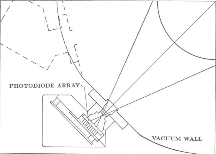
The light emission from the object is measured by means of a camera made up of a lens and a one dimensional photodiode array. The camera is focussed to project an image of the luminous object onto the sensor array. It is assumed that the camera is far away compared to the total size of the object, so that distortion is negligible and all image rays are approximately parallel. Consider the line passing through a point on the photodiode array and the optical center of the lens. The image intensity at that point of the photodiode array is proportional to the sum of the luminosities contributed by all object volume elements also lying on the line. For the assumed
10 element photodiode array, a single measurement obtains the projection of the
intensity distribution along one axis. If we consider the array values to be a set of 100 unknown quantities, we now have 10 equations in 100 unknowns. These are simply the following: P1 = 1(1, y) P2 O 1(2, y) P3 1 1(3, y) P 0 E oI(10, y)
where I(x, y) is the intensity of the object grid point at coordinate x, y. 90 more inde-pendent equations must be generated in order to solve for all 100 unknown intensities.
DETECTOR ARRAY
IMAGE PLANE
CAMERA
Figure 2.1
Geometry of Optical Tomography. The cylindrical object represents a luminous specimen. The intensity distribution across the plane indicated may be determined tomographically.
INTENSITY
Figure 2.2
View in the analysis plane. A one dimensional image is formed by the camera at each of several angular positions. Each image measures the projection of the intensity distribution along a single axis. A complete set of such images will allow the reconstruction of the original object
A new set of projections is generated when the object is rotated about its center by some angle 0. In this case, it is reasonable to assume that a set of 10 rotations equally spaced through 1800 might be sufficient to determine all 100 unknowns, since this would provide a total of 100 equations. It will be shown that this estimate is actually low by a factor of 7r/2. This indicates that, in order to provide a reasonable reconstruction of a 10x10 array, a series of at least 15 angular views is needed, each with a spatial resolution of less than 1/10 of the sample diameter.
Once we have determined a sufficient set of projection values, the task of solving the set of equations remains. One possibility is to solve the problem analytically; for the 10x10 cell reconstruction being considered, this would require the inversion of a 100x100 matrix. Although such an approach might seem reasonable in this case, a more typical reconstruction might involve a 500x500 pixel image array, requiring the inversion of a 250000x250000 matrix. In addition, it has been asssumed that the projection data is perfect, i.e. that it contains no noise. When noise is present, the matrix cannot be inverted since the noisy projections do not correspond to a unique solution. A proper reconstruction should in some sense describe the 'best fit' to the projection data. In general, an analytical solution is not considered; instead an approximate solution is found by one of several methods. The methods differ in their complexity, speed, ability to deal with sparse data, and sensitivity to noise. We will review some of the more commonly used methods below.
RECONSTRUCTION TECHNIQUES
The multiple one-dimensional angular views may be converted to a plane im-age through any of several reconstruction methods [Bu78]. The three most common techniques are:
1) Algebraic Reconstruction Technique (ART)
2) Filtered Back Projection (FBP)
3) The Method of Fourier Transforms (FT)
A new technique which has been applied to reconstruction problems recently is:
ALGEBRAIC RECONSTRUCTION
ART is an iterative process made up of three steps (Figure 2.3):
1) An trial image matrix, initially blank, is projected in the
direc-tions corresponding to the available projection data. We now have
a set of trial projections, and the set of real data. For the first
iteration, all trial projections are zero for all points.
2) For each angle in turn, the pair of one-dimensional pro-jection arrays are compared, and the difference between them is calculated point by point. This error matrix is then projected back across the image matrix after proper normalization. This insures that the image projection at that angle now agrees with the real data. This agreement is short-lived, since the next angle correction will change the image data.
3) The image matrix now contains the first approximation to
the final image. Steps (1) and (2) are now repeated. The image matrix should continue to improve as the error matrices decrease in magnitude. Clearly, if the image acquires values which are con-sistent with the real projection data, the error matrices will be zero and no further change will take place.
In general the data will not be perfect and so the iteration could be continued in-definitely. There is a problem with the technique, however. The image will usually slowly converge to an optimum solution and then it will start to diverge, especially if the data contains noise. For this reason, care must be taken to stop the iteration at
the proper point.
ART is conceptually simple, and is particularly effective for situations where a complete set of angular projection are not available. However, the calculation is slow, and data at all angles must be available from the beginning of the procedure. Other techniques act on one projection at a time, allowing data collection and calculation to be done simultaneously.
ORIGINAL OBJECT G = 90 PROJECTION
2 3
.3 4 7
4 6
0 W 0 PROJECTION
SECOND APPROXIMATION IMAGE
2 3 5
2 3 5
FIRST APPROXIMATION IMAGE
0 0 0 0 0 0 o = 90 ERROR ARRAY 4 6
G
0 ERROR ARRAY -2 12 2 3 4 Figure 2.3Algebraic Reconstruction Technique. Here, a 2x2 image (top left) will be re-constructed from its projections along two axes (0=0 and 0=90) A blank matrix is used as a first approximation to the image. The projections of the trial image are compared to the true projections, and the resulting error array is divided by 2 and added back to the trial iamge. The process is repeated for the second axis, yielding the original image. For larger arrays, projections are taken along a range of angles,
Back projection was the first method used for the reconstruction of a tomographic image. An image is built up by projecting each data array across an initially blank two-dimensional image matrix, and summing the contributions. Each projection is done at the angle at which the data was collected.
Since any object can be represented by a superposition of point objects, obtaining a clear reconstruction of a point image is all that is needed. The Figure 2.4 demon-strates the results of this method assuming a point object centered in the field of view. Each data projection is similar, consisting of a single central point. One projection array is back-projected in Figure 2.4b. The result is a narrow stripe across the image array. As subsequent back-projections are added, a star-shaped image is produced with a large central value. In the limit of infinite resolution and an infinite number of angular projections, the resulting shape is a 1/r cusp (Figure 2.4d). An arbitrary original object would reconstruct to a blurred image. A modification of the method is clearly necessary.
If the projections for a point object are to sum to zero outside of the central region, there must be some negative components to the arrays before they are back-projected. It can be shown that the original data arrays must be convolved with a filter function of the form:
F = 14,
lxi
< 1/2 (2.1)-- 1/X2, JxJ > 1/2
shown in Figure 2.4d. This filter function will result in projection arrays which con-tain a positive pulse and negative side lobes as shown. When these filtered projections are back-projected across the image array, the central pulses add constructively. Any point outside of the intersection region receives both positive and negative contribu-tions which sum to zero. This last property follows from the fact that the integral of the filter function is zero. Although there is theoretical justification for the above fil-ter function, other filfil-ter functions may be selected for purposes of edge enhancement, smoothing, etc.
The algorithm for filtered back projection has the advantage that data can be filtered and back-projected one angle at a time, therefore the system can be calculat-ing the partial solution while waitcalculat-ing for additional data to become available. The
a
t
C
INTENSITY RADIUSd
Figure 2.4Back Projection. Figure (a) represents a central point object projected on to four axes. When a single projection is projected back across a blank image figure
(b) results. In the limit of a large number of angles, the result of
projection/back-projection is a 1/r blur (d)
Amplitude Distance
a
Amplitude Din
in
II
',-N V
C
Figure 2.5Filtered Back Projection. Figure (a) shows the convolution function used for fil-tered back projection. An arbitrary projection (b) is convolved with the filter function
b
-,I
IN
algorithm is quick and relatively simple, and is the method used for the experimental results presented in the next chapter.
FOURIER RECONSTRUCTION
The Fourier Transform method of reconstruction is not as conceptually simple as the methods described previously. The Fast Fourier Transform algorithm is used to do in frequency terms what filtered back projection does in spatial terms. Instead of summing projections in image space, the Fourier Transforms of the projections are calculated, and these one-dimensional transforms are back-projected to form a two-dimensional frequency distribution. Particular frequency cutoff functions serve the purpose of the particular FBP filter functions. A two-dimensional inverse Fourier Transform of the frequency distribution produces the final image.
Although somewhat more mathematically sophisticated than the previous meth-ods, the Fourier technique is quite fast. Image quality is similar to that of Filtered Back Projection.
MAXIMUM ENTROPY
A relatively new technique developed for certain intractable problems [Ki83] has
been applied recently to the problem of image reconstruction. This method borrows from the formalism of statistical mechanics to search for a solution to a multiparameter fitting problem, which the problem of image reconstruction may be considered to be.
Given a set of N parameters which are to be varied in order to minimize some error function, several general methods are available. The most straightforward is to try all combinations of all possible parameter values. If there are more than a very small number of parameters, this method is far too slow. In the case of ten variables each with a range of only ten values, 1010 evaluations of the error function
are necessary.
A more practical method optimizes one parameter at a time, and iterates through
the parameter list until a minimum in the error function is found. This works if the parameters are reasonably independent, and there are no relative minima in the error function. Unfortunately, many real problems are not well behaved, and the error space is littered with spurious minima.
Most conventional searches rely on the change in an error function to determine the direction of parameter changes. If a given parameter change reduces the value of the error function, the changed parameter set is accepted as the starting point for the next step in the search. If the error function is increased, the parameter change is discarded. The ME technique differs in this respect. Here, a parameter change yielding an improved fit is still kept, but one which gives a worse fit may also be accepted with a probability given by a weighting factor of the form exp(-p/T) where
p is the change in the error function for the new parameter set. For large T, a poor
change in the parameter set will be accepted with high probability as long as it is less than 1/T in magnitude. For small T, the search will act more like a conventional method, with bad parameter changes being rejected.
The technique begins with an initial parameter set and a large value of the pa-rameter T. Random variations are made in the papa-rameter set; these random variation may be accepted or rejected according to the above criterion. After some number of variation steps, the parameter T is reduced in value, and the procedure is repeated. Eventually the problem converges to a solution at low T. The rate at which T is re-duced - the 'annealing schedule', must be determined for a particular set of problems. This method has been used for tomographic reconstruction by varying image pixel values and comparing the resulting image with the experimental data.
NOISE IN RECONSTRUCTED IMAGES
The nature of the tomographic reconstruction process must be considered when predicting the minimum limits on the detectability of trace elements in a matrix. With conventional X-ray fluorescence, this calculation is reasonably straightforward. We will briefly outline noise considerations for conventional x-ray fluorescence, then describe the limits imposed by the reconstruction process itself.
Three sources of noise must be considered for X-ray fluorescence:
1) Elastic scattering from the incident beam
2) Inelastic scattering from the incident beam
Figure 2.6 shows a typical spectrum produced from the analysis of iron distribu-tion in an organic specimen using a Si-Li detector with a resoludistribu-tion of 240 eV. Because the K edge of iron is at 7.1 keV, the fluorescence cross-section is at a maximum for an incident beam energy just above that value. An energy somewhat higher, 7.2 keV is used so that the elastically scattered beam is separated from the iron x-ray line at 6.4 keV. The inelastically scattered beam appears as a broadening of the elastic peak. The signal from scattering of the incident beam provides the primary source of background in a measurement of the iron signal. It is found that Si-Li detectors produce a uniform background which extends down from each peak in a spectrum, and which contains 3-5% of the peak intensity. For this reason, the background from the elastically and inelastically scattered peaks is greater than would be predicted from the detector resolution and peak spacing.
A minimally detectable quantity may defined as that concentration of material
which yields a signal just equal to the fluctuations in the background signal for a given detector. Since we are considering an x-ray counting technique, this may be expressed in terms of the signal count rate S, the noise count rate B, and the counting time t. Since the standard deviation of a count n is n1/2, we have the condition:
St = (Bt)1/ 2
S = (Blt)1/2
The required signal count rate, and therefore the required elemental concentration, decreases as 1/t1/2 for a fixed background count rate. Given a sufficiently long count-ing time, any arbitrary concentration could be seen. Different techniques can be compared if analysis time is assumed fixed, and typical incident fluxes are used.
A minimum concentration not explicitly dependent on counting time can be
derived from the condition that the signal count rate equal the background count rate. Although the concentration thus derived is not a true minimum, the result is useful for comparing different techniques, since the result is not dependent on counting times or beam flux, but only on background count rates. Since background signal is a smooth function of energy, the signal to background ratio is optimized by the use of a detector with a resolution equal to the x-ray line width. This limit can be approached with the use of crystal spectrometers.
sensi-Ul) 0 U
1
2
3
4
5
6
7
ENERGY (keV) Figure 2.6Fluorescence Spectrum: Iron in Carbon Matrix The spectrum of a honeybee with a 7.2 keV beam incident. The broad high energy peak is due to elastic and inelastic scattering of the incident beam by the organic matrix. A manganese peak is seen below the iron peak.
BEE2MCA.
Fe BEAM
1) The signal intensity is equal to the background generated by
secondary electrons in the matrix.
2) The incident projectile parameters have been optimized for the best
signal to noise ratio.
3) The detector has a resolution equal to the line width of the induced
x-ray.
Although the detectability limits for trace elements can be determined from back-ground considerations, other effects must be considered when an image is to be pro-duced tomographically. For images created by a conventional two-dimensional sur-face scanning technique, the statistical fluctuation in an image element containing
N counts is VN7. The statistical significance of a high count pixel is determined by comparison to the value of
vVN.
When the image is created tomographically, this simple statistical statement no longer holds.We will examine the effect of the reconstruction process by considering the case in which the background is small compared with the statistical
(N)1/2
uncertainty of the signal itself. It is assumed that the collected counts represent a real signal. The analysis assumes the use of the Filtered Back Projection method of reconstruction.A slice of thickness w through an object of diameter D is shown in Figure 2.8. An trace inclusion of iron is concentrated in a volume of dimension w3 at its center. Let the incident photon beam be square in cross-section, with a height and width
of w, and negligible divergence. We will consider the object to be divided into an
array of volume elements (pixels) of size w3. A tomographic analysis on this grid
would require v = D/w angular projections, each with a spatial resolution of w. The beam must therefore be scanned to D/w positions at each angular orientation. Here we have used the approximation that reconstruction of an v x v matrix requires v projections each with v values; this is correct to about a factor of 2.
The data collection proceeds by scanning the synchrotron beam in equally spaced steps across the specimen. At each step, the beam will induce x-ray emission from all pixels along the beam path. Some fraction of these induced x-rays will be detected. Any x-rays within the energy limits set for the particular trace element of interest will
105 Elcdron-induce KX-rays 10 -6.
g
1010--z
10-'0 Photon-induced KX- rays 10 20 30 40 50 Z in Carbon 'Motrix Figure 2.7The intrinsic sensitivity as a function of the sought-for trace element in a carbon matrix for three techniques of x-ray fluorescence analysis using: Upper curve, electrons of from 50 to 100 keV; middle curve, protons from .4 to about 2 MeV; lower curve,
photons whose energy is 1% above the binding energy of the K electrons of the sought-for species. [Gr83]
- D - )
PROJECTION 92
Figure 2.8
Tomographic Analysis of Single Inclusion. The reconstruction of an object with a single, central nonzero value results in a set of indentical projections (bottom). If the original measurement contains a noise component, the reconstruction process will add that noise to the entire image.
*6
'0'
oV
'4n
be counted and stored. In the case of the present specimen, some number (n) counts will be collected at that beam position which passes through the central pixel, and zero counts elsewhere (Figure 2.8). When the lateral scan is complete, an array of v projection values will have been determined. This array is stored, and the specimen is rotated through an angle of 7r/v. A new data set is collected at this angle, and for all angles up to 0 = 7r. The data collection will thus yield a set of similar projections each with a value of n N/nii counts in the central position, and zero elsewhere. The
v projections are then convolved with the filter function, then each filtered projection
array is back-projected across an initially blank image matrix, each at the angle cor-responding to its collection angle. As the filtered projections are superimposed on the image matrix, the central image pixel will accumulate a total count of approximately
N = nv. Points outside the central pixel will receive a positive contribution from
one projection, and negative contributions from all others. The resulting for image positions corresponding to a zero value in the original object is an avaerage value of zero. However, although the average value of the 'outside' pixels is zero, there is a fluctuation about zero. We will show that this results from the statistical fluctuation in the counts originating from the single central pixel.
The final reconstruction produces a value of N counts in the central point, made up of a superposition of v views each contributing N/v counts. The standard devia-tion of the contribudevia-tion of a single view is thus V/N/v. For any other pixel, the value of N/v will be added once, leaving a net average result of zero. The deviation from zero will be the sum of the deviations from the positive and negetive values:
6 = %/2N/v
Image positions which contributed no signal therefore have a variation in value which is 2 1/v times the noise fluctuation in the single central pixel. The results of computer simulations of point image reconstruction with statistical noise are shown in Figures 2.9-2.10
If the counts come from an extended source instead of a single pixel, we may sum the noise contributions from each contributing pixel in order to determine the effect on a non-contributing pixel:
2 N1 N2 N3
0.030 0.020 Nyje,, = 10 CV 0.010 Niews = 20-0.009 -0.008 0.007 '_ 0.006 a> 0.005 e 0.004 -= -- views = 30 0.003 Nview = 50 0 S0.002 Nviews =40 0.001 ' ' ' 0 5 10 15 20 25 30 Radius Figure 2.9
Statistical fluctuation in non-central points for specimen with single central inclu-sion. Data is shown for several values of angular resolution. Fluctuation is expressed as a fraction of central reconstructed amplitude, which is held constant at 1000 counts
0.0100 4J 0,0.0050 0.0010 0 0.0005 0 5 10 15 Radius 20 25 30 Figure 2.10
Statistical fluctuation in non-central points for specimen with single central in-clusion. Counts expressed as a fraction of central amplitude. Number of views is fixed at 50. The curves are labeled with the value of the central pixel for a single projection.
I=10
I = 100 I = 1000
2 (2 * total)
V
(2 * total) (2.2)
VV
Where the Ni are the reconstructed values over all contributing pixels. Of course, the sum could be taken over all image pixels, since all others are assumed to contribute an average value of zero. This noise contribution will add to the contributing pixels as well, and must be convolved with their /N noise to obtain the total noise.
For a low contrast image extending over the entire field, we may express the relative noise in terms of the average image value N and replace 'total' with v2 V,
yielding a noise over the image of:
U 2*total
N N2v
a 2v2N v
(2.3)
N N2v (2.3)
A low contrast image in which the pixel values are just equal to their statistical
fluctuation requires that
c/N =i, (2.4)
and so v=N; the total counts in the reconstructed pixel must be equal to number of angular views in the reconstruction, and so equal to the square root of the number of pixels in the reconstruction. In other words, the number of counts contributed by each pixel from a single angular view is equal to 1. The results of computer simulation of an extended image reconstruction with statistical noise is shown in Figure 2.11.
Clearly, the use of a reconstruction technique to produce an image does exact a price: for a low contrast image, the statistical noise in the final image is not equal to the square root of the image value, but is worsened by a factor of \,F. The relative fluctuation is that which would be expected from the counting statistics for a single view.
It is also clear that the effect of reconstruction on statistical noise depends on the image. For an image made up of a few small areas of high intensity, these areas have a relative statistical variation which is approximately equal to 1/v/ where N is the
0.50 1 A V M= 10 0.10 --1= 100 0.05 1= 1000 0 5 10 15 20 25 30 Radius Figure 2.11
Statistical fluctuation in a low contrast extended specimen. The result is ex-pressed as a fraction of the reconstructed value. All curves represent 50 view recon-struction, and are labeled with the value of the central pixel for a single projection.
reconstructed count in that area. Images which contain large uniform areas will have relative variations on the order of N/v/N.
CHAPTER 3


![[PDF] Cours de systèmes d’exploitation informatique PDF - Cours maintenance PC](data:image/gif;base64,R0lGODlhAQABAIAAAP///wAAACH5BAEAAAAALAAAAAABAAEAAAICRAEAOw==)