Three-dimensional V
P
and V
P
/V
S
models of the upper crust in the
Friuli area (northeastern Italy)
G. F. Gentile,
1 G. Bressan,2 L. Burlini3 and R. De Franco4
1 Osservatorio Geofisico Sperimentale, Dip. OGA, Borgo Grotta Gigante 42/c, 34100 Sgonico, T rieste, Italy. E-mail: [email protected] 2 Osservatorio Geofisico Sperimentale, Dip. CRS, CPI Cussignacco, 3100 Udine, Italy. E-mail: [email protected]
3 ET H Zentrum, Rock Deformation L ab, Sonneggstrasse 5, 8092 Zu¨rich, Switzerland. E-mail: [email protected] 4 Consiglio Nazionale delle Ricerche, IRRS, V ia Bassini 15, 20133 Milano. Italy. E-mail: [email protected]
Accepted 1999 December 9. Received 1999 November 29; in original form 1999 March 1
S U M M A R Y
3-D images of P velocity and P- to S-velocity ratio have been produced for the upper crust of the Friuli area (northeastern Italy) using local earthquake tomography. The data consist of 2565 P and 930 S arrival times of high quality. The best-fitting V
P and VP/VS 1-D models were computed before the 3-D inversion. VP was measured on two rock samples representative of the investigated upper layers of the Friuli crust. The tomographic V
P model was used for modelling the gravity anomalies, by converting the velocity values into densities along three vertical cross-sections. The computed gravity anomalies were optimized with respect to the observed gravity anomalies. The crust investigated is characterized by sharp lateral and deep V
P and VP/VS anomalies that are associated with the complex geological structure. High VP/VS values are associated with highly fractured zones related to the main faulting pattern. The relocated seismicity is generally associated with sharp variations in the VP/VS anomalies. The V
Pimages show a high-velocity body below 6 km depth in the central part of the Friuli area, marked also by strong VP/VS heterogeneities, and this is interpreted as a tectonic wedge. Comparison with the distribution of earthquakes supports the hypothesis that the tectonic wedge controls most of the seismicity and can be considered to be the main seismogenic zone in the Friuli area.
Key words: earthquakes, gravity anomalies, seismotectonics, tomography.
3-D P-velocity model was characterized by strong lateral
I N T R O D U C T I O N
heterogeneities connected with a complex tectonic pattern. In particular, Amato et al. (1990) showed that most of the 3-D joint inversion for hypocentres and velocity structure
(Thurber 1983; Eberhart-Phillips 1986; Evans et al. 1994) is seismicity is localized within a southward-verging high-velocity body (V
P≥6.2 km s−1), more than 5 km deep. Subsequently, a suitable method for investigating the regional tectonics and
seismogenic characteristics of an area. The computed velocity Bressan et al. (1992), using the same tomographic inversion method but with a different set of data combined with gravi-images provide useful information on the relationship between
superficial and deep tectonics, fault zones and the variation in metric inversion, confirmed the previous results and interpreted the high-velocity body as the main seismogenetic zone of the seismic properties in the crust associated with the geological
setting. Comparison with seismicity patterns provides the basis Friuli area. All these investigations were based on P-wave analogue data.
for a seismotectonic model explaining the relationships between
the various structural units and the earthquake nucleation In the present study we have computed 3-D V
Pand VP/VS models, using better quality data (digitally acquired waveforms) zones.
The upper crustal structure of the Friuli area (north- from local earthquakes as recorded by the Friuli–Venezia Giulia local seismic network in order to investigate in detail eastern Italy) was first investigated by Amato et al. (1990)
using local source tomography techniques. Their tomographic the main tectonic features of the area.
457 © 2000 RAS
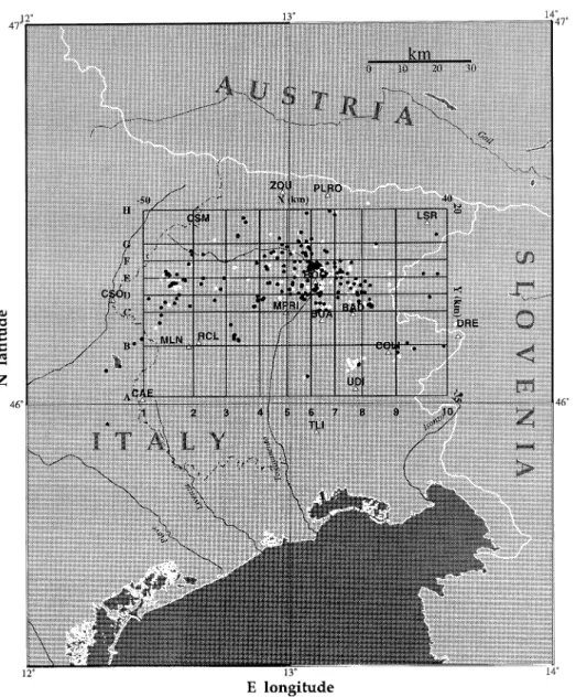
Figure 1. (a) Schematic geological map of the eastern Southern Alps. Symbols: (a) Hercynian low metamorphic basement (Ordovician– Carboniferous); ( b) Palaeocarnic non-metamorphic chain (Upper Ordovician–Carboniferous) and Upper Carboniferous–Lower Permian covers; (c) Permo-Mesozoic, mainly carbonatic, successions; (d) flysch (Upper Maastrichtian–Middle Eocene) and molassic sequence (Miocene); (e) Quaternary alluvial deposits and moraines; (f ) thrust; (g) subvertical fault. UD: Udine; TS: Trieste. Inset (b) Early syn-sedimentary faults reactivated during the Neoalpine compressions: PC–VB (Pieve di Cadore–Val Bordaglia fault); T–BC (Tramonti–But Chiarso` fault); D–I (Dogna–Idria fault); IL (Insubric Line); ML (Mojstrana–Ljubljana fault). The tectonic pattern outlined by these master faults consists of two indented tectonic wedges, named, respectively, inner and outer wedge. The grid of 3-D V
Pand 3-D VP/VS inversions is shown (modified from Bressan et al. 1998).
Figure 2. Interpreted geological cross-section 7 N–S of Fig. 1. Symbols: (a) Quaternary and Cenozoic units; ( b) Mesozoic units; (c) Palaeozoic units; (d) fault.
The tectonic constraints of both wedges are NE–SW- and
G E O L O G I C A L A N D S T R U C T U RA L
NW–SE-orientated palaeofault systems (PC–VB, T–BC, D–I,
SE T T I N G
ML faults in Fig. 1), active as strike-slip faults from Palaeozoic to Middle Eocene times, which were re-activated during the com-The geological units of the Friuli area (Fig. 1) consist mainly
of sedimentary rocks of Palaeozoic to Quaternary age. The pressional Cenozoic phases. The Mesoalpine (Dinaric) NE–SW compression generated NW–SE-orientated thrusts during the Palaeozoic rocks are made up of limestones, terrigenous and
volcanic deposits. Limestones and carbonate rocks characterize Middle–Late Eocene. A Middle Miocene–earliest Pliocene N–S-orientated compression followed, causing severe shorten-the Jurassic–Cretaceous period, while shorten-the prevalent Cenozoic
and Quaternary deposits are flysch and molasse. The study ing of the central area by means of south-verging thrusts and backthrusts. The palaeofault systems acted as strike-slip faults. area is characterized by a complex tectonic pattern (Fig. 1),
resulting from the superposition of several Cenozoic-age Later, a Pliocene NW–SE-orientated compression generated trending thrusts and folds, re-activating the NE–SW-tectonic phases. The structural setting consists of two indented
trapezoidal wedges, the outer containing the inner ( Venturini orientated palaeofaults as inverse faults. Neotectonic activity was intense mostly in the southernmost belts of the inner and 1991).
Figure 3. Location of the 3-D inversion grid: the triangles indicate the seismic stations; black dots, the earthquakes used for the VPinversion; and white dots, those used for the VP/VS inversion. South to north grid nodes are marked as letters A, B, C, D, E, F, G, H, corresponding to Y (km) distance. West to east grid nodes are marked as numbers 1, 2, 3, 4, 5, 6, 7, 8, 9, 10, corresponding to X ( km) distance. (See text).
outer wedges. A schematic geological cross-section of the 1348 event with epicentral intensity I
0=IX MCS (Mercalli– Cancani–Sieberg scale), the 1511 event (I0=IX MCS), the central part of the study area is shown in Fig. 2.
The present state of tectonic stress, as inferred from the focal 1928 event (I
0=IX MCS) and the 1976 event (I0=X MCS, M
L=6.4). mechanisms of earthquakes (Bressan et al. 1998), appears to
be significantly conditioned by the geometry of the indented wedges. It is characterized by a general compressional state of stress with a strike-slip stress state localized in the eastern
3 - D T O MO G R A P H Y
part. The maximum compressional axis of stress is orientated from NW–SE in the western part to N–S in the eastern part
Inversion method and data set
of the area.
The seismicity is strongly focused in the central part of the The 3-D V
Pand VP/VS tomographic images of the upper crust are obtained using Thurber’s (1983) method of joint inversion Friuli area, with the maximum density of earthquakes occurring
between 7 and 11 km depth. This area has been affected in the for hypocentres and 3-D velocity structure from local earth-quakes. The computer code (Evans et al. 1994) is past by destructive earthquakes (Slejko et al. 1989) such as the
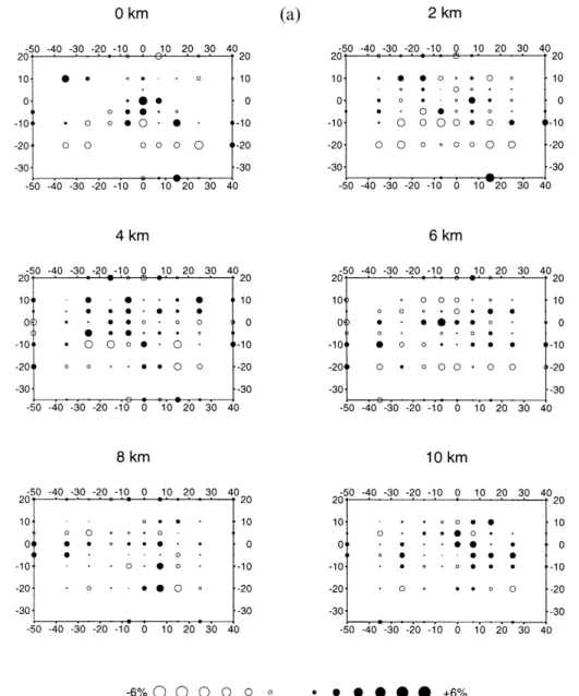
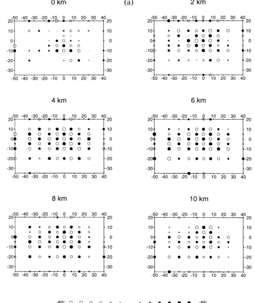
Figure 4. Results of the 3-D V
Pinversion at six depth slices (0, 2, 4, 6, 8 and 10 km). The X ( km) and Y ( km) distances are marked (see Fig. 3). (a) P-velocity images; (b) diagonal elements of the resolution matrix; (c) standard error.
used. A 1-D starting velocity model is assigned to the nodes vertical 1 Hz seismometer, except stations CAE, DRE and ZOU which are equipped with three-component 1 Hz seismo-of a 3-D grid and the velocity value at any other point is
obtained by linear interpolation between the nodes. The travel- meters. Since June 1995, station BAD has been equipped with a 3-D seismometer. From 1988 to April 1994 the sample rate time from hypocentre to station is calculated by a
pseudo-bending method (Um & Thurber 1987). The solution is then was 360 sps on vertical sensors and 120 sps on each of the 3-D sensors, with a dynamic range extending up to 96 dB and obtained by an iterative procedure, solving for hypocentre
location and calculating the velocity of the medium, with a 10-bit digitizing. The network was upgraded in April 1994 to include digital signal processing with a 16-bit digitizer, 120 dB damped least-squares approach.
The 3-D V
Pand VP/VS inversions are based on the arrival of dynamic range and a sampling rate of 62.5 sps.
The area investigated is represented digitally by a grid times of P and S waves of local earthquakes, recorded by the
Friuli–Venezia Giulia seismic network (Fig. 3). The seismic extending 90 km in the west–east direction (west to east grid nodes at X=−50, −35, −25, −15, −7, 0, 7, 15, 25, 40 km) network consists of 15 short-period seismometers, with a digital
acquisition system and a trigger algorithm for event detection. and 55 km in the south–north direction (south to north grid nodes at Y=−35, −20, −10, −5, 0, 5, 10, 20 km). The depth Data are sent via a telemetry radio link to the acquisition
centre at UD (Udine, Fig. 1). All stations are equipped with a grid spacing is Z=0, 2, 4, 6, 8, 12, 15 km. The coordinates of
the grid centre are latitude 46°20∞N and longitude 13°05∞E.
Inversion procedure
The horizontal mesh of the grid is finer in the central part to
give an approximately homogeneous ray coverage within the Given that the S-wave data are of poorer quality and fewer in number than the P-wave data, we started by constructing a blocks. The data set consists of local earthquakes with local
magnitude ranging from 1.3 to 4.3, recorded by the seismic reliable 3-D V
P model and then inverting for VP/VS values, based on the results of the 3-D V
Pmodel. network from 1988 to 1997, located with a71program
(Lee & Lahr 1975), with GAP ( largest azimuthal separation The reliability of the results obtained with linear tomo-graphic inversion depends on the initial reference model. between stations)≤180°. The 3-D V
Pinversion was obtained
using 2565 P-wave arrivals from 224 events, with an estimated Kissling et al. (1994) showed that an inappropriate initial reference model could significantly affect the quality of the picking accuracy of±0.05 s. The data set for the 3-D VP/VS
model consists of 930 S-wave arrival times from 136 earth- tomographic images. We therefore followed the Kissling et al. (1994) approach by obtaining an initial reference model (the quakes, most of them recorded with the upgraded acquisition
system, which allows a picking accuracy of ±0.1 s for 3-D minimum 1-D model ), using the program (Kissling et al. 1995).
seismometers and±0.15 s for vertical seismometers. The
earth-quakes for the VP/VS model were carefully selected by visual An a priori P-velocity model of the Friuli area with constant-velocity layers was compiled using existing refraction seismic inspection to ensure a significant number of S arrival times.
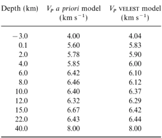
Table 1. 1-D VP a priori model and the minimum 1-D VP model
data (Pagini 1995). The minimum 1-D V
P model was then computed with the program. The first layer (−3.0 to 0.1 km computed with the program by inverting for
hypo-depth) includes all the seismic stations.
centres every iteration, and inverting station delays and velocity values every second iteration until the total RMS value (root
Depth (km) V
Pa priori model VP model
mean square misfit of traveltime residuals) reduced significantly
( km s−1) (km s−1)
and stabilized. Table 1 shows the a priori and the calculated
minimum 1-D models. The layer at negative 3 km depth has −3.0 4.00 4.04 been included to account for the Earth’s topography. The 0.1 5.60 5.83 damping value for the 3-D inversion is 10, selected following 2.0 5.78 5.90
4.0 5.85 6.00
the empirical approach of Eberhart-Phillips (1986) to give
6.0 6.42 6.10
both low data variance and low standard error. The effect of
8.0 6.46 6.12
topography in the 3-D inversions has been considered by
10.0 6.40 6.37
including the elevation of the stations.
12.0 6.32 6.29
The 3-D RMS residual is 0.203 s. Fig. 4(a) shows the V
Pimages 15.0 6.67 6.42
at six depth slices. The diagonal elements of the resolution
22.0 6.43 6.44
matrix and the standard error are shown in Figs 4(b) and (c), 40.0 8.00 8.00 respectively. Since the resolution is also controlled by the ray
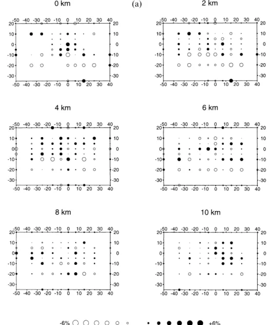
Figure 5. Results of the 3-D VP/VS inversion at six depth slices (0, 2, 4, 6, 8 and 10 km). The X (km) and Y (km) distances are marked (see Fig. 3). (a) P- and S-velocity ratio images; ( b) diagonal elements of the resolution matrix; (c) standard error.
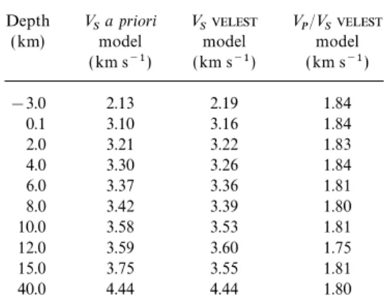
Table 2. 1-D VSa priori model, the minimum 1-D VSmodel and the
density, the best resolution is found in the central part of the
1-D VP/VS model computed with the program.
grid at depths from 2 to 6 km, where the station coverage is denser and the number of earthquakes is larger. The poor
Depth V
Sa priori VS VP/VS
resolution in other sectors of the grid is explained by the
( km) model model model
poor density of earthquake ray paths. ( km s−1) ( km s−1) ( km s−1) The VP/VS minimum 1-D model; that is, the initial reference
model for 3-D VP/VS inversion, was also computed with the −3.0 2.13 2.19 1.84
0.1 3.10 3.16 1.84
program (Kissling et al. 1994). The a priori 1-D model
2.0 3.21 3.22 1.83
consists of the average V
P computed for each layer from the 4.0 3.30 3.26 1.84 calculated 3-D V
P model, and VS values taken from Riggio 6.0 3.37 3.36 1.81
et al. (1987) and Fah et al. (1993). The earthquakes were
8.0 3.42 3.39 1.80
relocated by fixing the V
Pvalues and inverting for the shear 10.0 3.58 3.53 1.81
wave velocity only. The a priori V
Smodel and the calculated 12.0 3.59 3.60 1.75
minimum VP/VS 1-D models are shown in Table 2. The 15.0 3.75 3.55 1.81
40.0 4.44 4.44 1.80
damping value for the 3-D VP/VS inversion, based on the Eberhart-Phillips (1986) method, is 5. The 3-D VP/VS data were inverted by fixing the V
Pvalues as obtained from the 3-D images of the diagonal-elements resolution and the standard V
Pmodel and allowing hypocentre relocation. The 3-D RMS error. The central part of the area shows higher resolution at residual is 0.274 s. The plan-view maps of the VP/VS anomalies depths from 2 to 6 km, as expected from the station coverage
and distribution of earthquakes. are shown in Fig. 5(a). Figs 5(b) and (c) are, respectively, the
Figure 5. (Continued.)
Since most of the S arrivals are taken from vertical sensors, The calculated 3-D VP/VS model (Fig. 5a) shows values decreasing with increasing depth, a reasonable trend consistent the VP/VS inversion is subject to larger errors than the VP-only
inversion. The picking of S waves from vertical sensors is less with the closing of microcracks under increasing confining pressure.
accurate than for the P arrivals because they are partially obscured by the P-wave signal. However, a more serious problem in identifying shear waves from vertical instruments
Resolution analysis
(Thurber & Atre 1993) arises from S-to-P converted waves,
which arrive before the true S wave and which can be wrongly Following the approach of Zhao et al. (1992), we analysed how the true velocity images were reconstructed in the inverted identified as the direct signal. This can result in artificially
low values of VP/VS, especially in areas with unconsolidated velocity images using the checkerboard resolution test (CRT) and restoring resolution test (RRT).
sediments overlying rock units with sharp velocity contrasts.
This effect is negligible in the present study because only two The goal of the CRT is to investigate the adequacy of the ray coverage and the resolution. The checkerboard model was vertical stations (TLI, UDI) are located on unconsolidated
sediments (Fig. 3), and the number of S arrival times from constructed by assigning to the 3-D grid nodes positive and negative fractional V
P (6 per cent) and VP/VS (3.5 per cent) these sites used in the VP/VS inversion is 24, a small fraction
of the total employed phases (930). perturbations. Figs 6(a) and ( b) show V
Figure 6. Fractional (a) VPand ( b) VP/VS perturbations (in per cent), obtained with the tomographic inversion at six depth slices (0, 2, 4, 6 and 8 km). The X (km) and Y (km) distances are marked (see Fig. 3).
perturbations in per cent, obtained with the 3-D inversion. normal distribution, as in the real data set, were added to the calculated synthetic arrival times. A restored image was con-Figs 7(a) and ( b) are, respectively, the images of V
Pand VP/VS synthetic checkerboard inversions. The V
P checkerboard structed by inverting the synthetic data. The RRT VPimages (Fig. 8a) show that the tomographic images are well restored pattern is well reconstructed in the central part of the area for
layers at 2, 4, 6 and 8 km depth, with the best reconstructed for layers at 2, 4, 6 and 8 km depth, while the 3-D inverted VP/VS images are less well restored (Fig. 8b). The best restored patterns at 4 and 6 km depth. The resolution decreases at
10 km depth because of the low number of quakes, with VP/VS tomographic images from the RRT are in the central parts of the layers at 4 and 6 km depth. The average deviation consequent relatively poor sampling of nodes by ray paths.
The checkerboard pattern is not correctly reconstructed at from the initial locations of the hypocentre locations obtained with the RRT is 0.3 km.
0 km depth because of uneven sampling of ray paths. The resolution of the VP/VS images is lower than that of the VP images, and the best reconstructed patterns are at 4 and
D I S C U S SI O N
6 km depth.
The goal of the RRT is to check how errors in the data set
Tomographic results
influence the inverted images and the relocation of the
earth-quakes. The 3-D tomographic images obtained were considered Based on the 3-D VP/VS model, we relocated 415 events that occurred within the study area during the period 1993–1996, as the synthetic model of the RRT. Random errors with a
Figure 6. (Continued.)
in order to give an improved representation of the seismicity anomalies indicates a crystalline basement at a depth of nearly 10 km, affected by south-verging thrusting and detached from pattern for comparison with the calculated tomographic model.
The distribution of V
P and VP/VS anomalies is charac- the overlying Mesozoic cover. The resolution of the tomo-graphic V
Pand VP/VS models at depths greater than 10 km is terized by marked lateral and depth variations (Figs 9a to d),
reflecting structural heterogeneities (Fig. 1). Low P velocities poor and does not allow detailed images to be constructed. However, this zone is characterized by V
P values of around (V
P=5.4–5.8 km s−1) and high VP/VS values (1.82–1.85) are
related to superficial molasse and flysch deposits in the southern 6.3–6.5 km s−1, and VP/VS ratios range from 1.75 to 1.80. As expected, VP/VS values decrease with depth since cracks sector of the investigated area. Mesozoic limestones and
dolomitic rocks, which constitute the main portion of the close with increasing pressure (O’Connell & Budiansky 1974). The near-surface high VP/VS values could result from the investigated crust, are characterized by a wider range of P-wave
velocities (5.9–6.6 km s−1) and VP/VS values (1.78–1.88). VP presence of water-saturated cracks, while the anomalously high VP/VS values (1.84–1.90) at depths greater than 3 km are values between 6.0 and 6.5 km s−1 and VP/VS values in the
range 1.75–1.82 below 5 km depth in the northern sector could attributed to highly fractured zones.
The most important feature revealed by the tomographic be related to the Palaeozoic units (terrigenous sediments,
lime-stone deposits, volcanic and low-grade metamorphic rocks). images is a high-velocity zone (V
P≥6.2 km s−1), bounded by sharp lateral and vertical velocity variations and located at According to Cati et al. (1987), the pattern of magnetic
Figure 7. Results of the checkerboard resolution test (CRT) for (a) VPimages and ( b) V
P/VS images. The X (km) and Y (km) distances are marked (see Fig. 3).
about 6 km depth in the central part of the inner tectonic shown in Fig. 9(c). All the earthquakes characterized by thrust focal mechanisms are located at the southern border of the wedge (Figs 9a to d). Its base is not clearly resolved, but the
boundaries of this zone are characterized by sharp VP/VS high-velocity bulge.
The E–W-orientated tomographic images (Fig. 9d) show variations. The shape of the high-velocity zone is not regular.
This is particularly evident in Fig. 9(d), where the high-velocity evidence of the western border of the inner tectonic wedge, marked by the Tramonti–But Chiarso` fault. The Tagliamento– body deepens towards the east. Most of the relocated
earth-quakes occur within or near the high-velocity body and along Osoppo strike-slip faults are marked by sharp lateral V Pand VP/VS changes in the central part of the inner tectonic wedge the high-VP/VS anomaly gradients (Figs 9a to d). We interpret
this tectonic structure to be the result of the severe crustal and clearly affect the geometry of the high-velocity zone. There is no clear evidence of correlation between the Idria–Dogna shortening caused by the Middle Miocene–earliest Pliocene
N–S-orientated compression (Venturini 1991). The VP/VS fault and the tomographic images because of poor ray coverage in this zone. The earthquake clustering that is noticeable in heterogeneities probably result from deformation along faults
affecting the high-velocity body. The stronger shocks of the the western part of Fig. 9(d) consists largely of the swarm that occurred from 1996 January to June, with main shock local 1976 sequence (Barbano et al. 1985), the most important
Figure 7. (Continued.)
Excluding effects due to high temperatures, which are not has resulted in a complex 3-D deformation pattern, with discontinuous blocks and bulges marked by rapid spatial expected from the geothermal environment of the area (average
heat flow 50–60 mW m−2, Cataldi et al. 1995), the high VP/VS variations in V
P and VP/VS values. The high-velocity body is taken to represent the more brittle and stronger parts of the values at depth are attributable to a high degree of fracturing
and high fluid pressure. Generally, we relate the sharp lateral seismically active layers and is considered to be the main seismogenetic zone.
VP/VS variations to the effects of faulting. The fluid overpressure can cause chemical effects, such as stress corrosion and pressure solution, with subsequent concentration and enhancement of local stresses, favouring the nucleation of earthquakes (Zhao
Experimental VP measurements
& Negishi 1998).
Generally, the overall V
P and VP/VS pattern reflects the For comparison with the tomographic results, laboratory measurements of P velocity were performed on samples complex tectonic-structural setting, resulting from the
super-position of three main tectonic phases ( Venturini 1991). collected in the ‘Dolomia Principale’ (dolomitic rock) and the ‘Calcare of Dachstein’ ( limestone) units. These lithologies Each tectonic phase, characterized by different orientations of
the principal axes of stress, inherited the deformations of the are representative of the Mesozoic units that constitute most of the crustal rocks in the study area.
Figure 8. Results of the restore resolution test (RRT) for (a) V
Pimages and ( b) VP/VS images. The X (km) and Y (km) distances are marked (see Fig. 3).
The velocity of compressional elastic waves was measured We computed the distribution of V
P, density and temperature with depth for a simplified lithological cross-section derived at confining pressures of up to 300 MPa on cores of 26 mm in
diameter and 35–55 mm in length, using the pulse transmission from Castellarin et al. (1979) (Fig. 11). We calculated geo-therms using a finite difference algorithm (1-D model) with the technique (Birch 1960). Sample preparation and details of the
technique used are the same as in Burlini et al. (1998). Bulk parameters listed in Table 3, assuming a temperature of 273 K and a heat flow of 50 mW m−2 at the surface. For the lower density was determined from weights. The confining pressure/
velocity relations are shown in Fig. 10. The non-linear part of crust and the upper mantle we also used a second temperature derivative. The temperature obtained at each depth level was the curve is generally interpreted as being due to crack and pore
closure (Birch 1961), while the linear part (at high pressure) used to calculate the effective density in dry conditions, using the pressure and temperature derivatives, and thus the pressure reflects the intrinsic seismic properties of the rocks, that is
the crack-free matrix properties, which correspond to the at depth. These pressures and temperatures were used to calcu-late the seismic velocity at each depth level based on the experi-maximum velocities possible for the rock type under
consider-ation. The maximum velocity at high confining pressure is mentally determined velocities and their pressure derivatives. For the temperature correction of V
P we took derivatives as 6.0 km s−1 for the limestone, and 6.9 km s−1 for the dolomitic
Figure 8. (Continued.)
Table 3. Thermal conductivity and its pressure and temperature derivatives, heat production, density and its pressure and temperature derivatives used to calculate the geotherm. These parameters were taken from a variety of sources (Haenel et al. 1988; Fountain et al. 1987 and references therein), and applied to the lithological section of Friuli with the same considerations as reported in Burlini (1992).
Rock type Thermal dk/dP dk/dT Heat Density dDensity/dP dDensity/dT
(model ) conductivity k (W m−1 K−1 Mpa−1) (W m−1 K−2) production (Mg m−3) (Mg m−3 Mpa−1) (Mg m−3 K−1)
(W m−1 K−1) (W m−3) Mesozoic limestones 6.52 4.5×10⁻⁴ 6.8×10⁻⁴ 8.0×10⁻⁷ 2.66 4.0×10⁻⁴ 5.0×10⁻⁵ Dolomitic rocks 6.52 4.5×10⁻⁴ 6.8×10⁻⁴ 8.0×10⁻⁷ 2.76 4.0×10⁻⁴ 5.0×10⁻⁵ Palaeozoic rocks 2.20 4.5×10⁻⁴ 4.5×10⁻⁴ 1.2×10⁻⁶ 2.66 4.0×10⁻⁴ 5.0×10⁻⁵ Quartzitic basement 4.30 4.5×10⁻⁴ 4.0×10⁻⁴ 1.2×10⁻⁶ 2.66 1.0×10⁻⁴ 5.0×10⁻⁵ Upper crust 3.28 4.5×10⁻⁴ 5.0×10⁻⁴ 1.2×10⁻⁶ 2.66 4.0×10⁻⁵ 1.7×10⁻⁵ Middle crust 3.38 2.0×10⁻⁴ 5.0×10⁻⁴ 2.0×10⁻⁹ 2.80 3.5×10⁻⁵ 1.7×10⁻⁵ Lower crust 6.138 2.0×10⁻⁴ 9.15×10⁻³ 1.2×10⁻⁸ 2.90 3.0×10⁻⁵ 5.0×10⁻⁵ Upper mantle 6.138 2.0×10⁻⁴ 4.31×10⁻³ 2.0×10⁻⁹ 3.34 2.5×10⁻⁵ 6.0×10⁻⁵
(a)
(b)
(c)
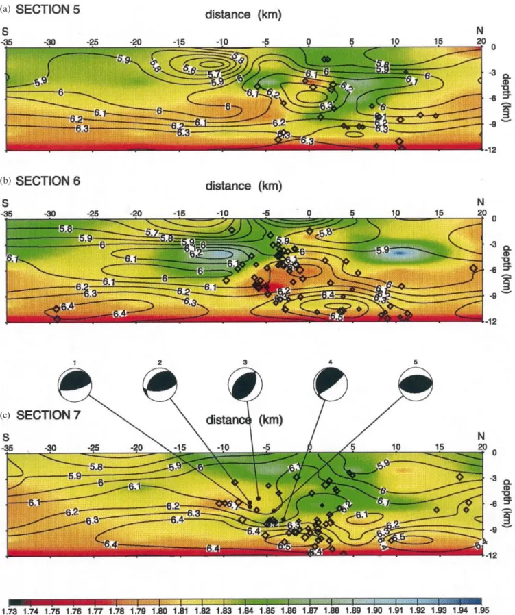
Figure 9. Vertical cross-sections of the 3-D VPand 3-D V
P/VS images. (a) section 5; (b) section 6; (c) section 7; (d) section E. The VP values are shown as contour lines. The VP/VS values are plotted in graded colours in (a) to (c), and in grey tones in (d). Diamonds indicate the positions of the relocated 415 earthquakes as calculated from the 3-D V
P/VS model. The focal mechanisms of the strongest earthquakes of the 1976 sequence are shown in section 7: (1) May 6, M
L=6.4; (2) September 11, ML=5.1; (3) September 15 ML=5.8; (4) September 15, ML=4.7; (5) September 15, M
L=6.1. On section E, the traces of the main faults are shown: (a) Tramonti–But Chiarso` fault; (b) (c) Tagliamento–Osoppo fault system; (d) Dogna–Idria fault. The locations of the cross-sections are shown in Figs 1 and 3.
Figure 9. (Continued.)
Figure 11. VP, density and temperature with depth calculated for the Figure 10. Confining pressure/velocity relations of two cores of Friuli Friuli section. V
Pis in km s−1, density in Mg m−3 and temperature in limestone cut parallel to layering (two mutually orthogonal directions, hundreds of°C. A simplified lithological cross-section derived from 1 and 2) and one core of Friuli dolomia cut normal to layering, as Castellarin et al. (1979) is considered: mainly limestones (from surface determined by laboratory measurement. Open symbols are increasing to 5 km depth); mainly dolomitic rocks (5–8 km depth); Palaeozoic pressure measurements, full symbols are decreasing pressure rocks (8–11 km depth); quartzitic basement (11–12 km depth); upper
measurements. crust (12–15 km depth); middle crust (15–25 km depth); lower crust
(25–31 km depth); upper mantle.
Since the 3-D V
Pinversion is best resolved from the surface density of the limestones ranges from 2.64 to 2.69 Mg m−3, while the computed density of the dolomitic rocks varies from to 8 km depth in the central part of the study area, we
examined the V
P/depth profile evaluated from laboratory data 2.79 to 2.82 Mg m−3. in this depth range for comparison with tomographic data.
The V
P values (about 6 km s−1) from the surface to 5 km Gravity modelling
depth correspond to the average V
Pvalues obtained with the
3-D inversion for this depth. The step at 5 km depth and The tomographic images were used for modelling Bouguer gravity anomalies, provided as digital data on a 3×3 km grid the increase in V
Pup to 6.8 km s−1 are in agreement with the
presence of the high-velocity body, supporting the inter- (Fig. 12) by Cassano et al. (1989). 2-D gravity models were constructed along tomographic sections 5, 7 and E of Fig. 9. pretation that the high-velocity body, or at least its uppermost
Figure 12. Bouguer anomaly contour map (5 mgal contour interval, reduction density 2.4 Mg m−3). The grey box indicates the tomographic study area. The modelled gravity lines along sections 5, 7 and E (see Figs 1 and 9) are shown.
Figs 13(a), ( b) and (c), respectively. The P-velocity values were tomography. The minimum density values (2.55 Mg m−3) of these layers are due to the presence of the shallow flysch and resampled along each section using a linear interpolation
algorithm (De Boor 1978) with meshes spaced 2.5 km hori- molasse sediments (maximum thickness 2.5 km) of the Friuli plain (Fig. 2). The maximum positive variations (0.06 Mg m−3) zontally and 1 km in depth. The P velocities were converted
into densities using the velocity–density relationship of Zelt & are found in the shallow part of the modelled section 5, between 0 and 10 km distance, and are associated with density Smith (1992). The arithmetic mean density was calculated
from the four density values of each mesh. The gravity response value of about 2.75 Mg m−3, appropriate to the Mesozoic rocks. Fig. 13(c) shows the gravity response modelled along was calculated with the Talwani algorithm (Telford et al. 1990),
using 2.85 Mg m−3 as background density. The model also the E–W-orientated tomographic section E. The mean residual of the initial model is 4.5 mgal, and the optimized density includes layers representing the upper crust extended to the top
of the lower crust (2.8 Mg m−3), the lower crust (2.91 Mg m−3) model shows a mean residual of 0.8 mgal. The most noticeable difference between the computed and the observed gravity and the upper mantle (3.10 Mg m−3) as derived from Italian
Explosion Seismology Group and the Institute of Geophysics, anomalies is found in the 30–40 km distance range, where the tomographic images show poor resolution because of poor ETH Zurich. (1981).
The initial computed gravity anomalies and the observed sampling of the seismic ray paths. The other minor gravity discrepancies observed in the gravity profiles may well be due N–S sections (Figs 13a and b) display a high degree of
correlation. The mean residuals of the initial computed gravity to local variations in the velocity–density relationship used. The prevalent geological unit consists of alternating Mesozoic anomalies are 4.2 mgal (section 5) and 3.8 mgal (section 7).
Optimized density models, obtained using the least-squares limestones and dolomitic rocks (Fig. 2). Considering the results from laboratory measurements and the distribution of inversion (More 1977), show mean residuals of 0.3 mgal for
both sections. The maximum negative variations (−0.08 Mg m−3 VP/VS anomalies, our interpretation is that the strong density variations seen in the gravity models for the crustal layers and−0.06 Mg m−3) of the optimized density model with respect
to the initial density model are observed in the superficial investigated is due to fracturing and a change in lithology from limestones to dolomitic rocks.
layers of the distance range −25 to −15 km for both N–S
sections. This disagreement could be due to the poor sampling Fig. 14 shows a map of the horizontal gradient modulus computed from the Bouguer anomaly data. The high-gradient of the shallow structure, which is not fully resolved by the
Figure 13. Gravity models of sections 5 (a), 7 ( b) and E (c). Upper panel: anomaly profiles. Lower panel: density model with values in Mg m−3. The contour values of density variation of the optimized models are shown. In the gravity modelling a layer with density 2.8 Mg m−3 is included from 12 km depth to the lower crustal boundary. The lower crustal boundary is modelled with a north-dipping plane, located at 25 and 19 km depth from the surface, respectively, at the northern and southern edges of the tomographic grid. The density assigned to this layer is 2.91 Mg m−3. The upper mantle boundary is marked with a north-dipping plane located 40 and 35 km depth from the surface, respectively, at the northern and southern edges of the tomographic grid. The density is 3.10 Mg m−3.
zone (>5 mgal km−1) corresponds to the boundary between around the tectonic wedge, which we consider to be the main seismogenic zone of the area. In accordance with laboratory the Friuli plain and the South-Alpine thrust belts. This zone is
orientated NE–SW in the western part of the study area and V
Pmeasurements performed on representative rock samples of the sedimentary crust, we relate the increase in V
P at the E–W in the central part, marking the limits of the high-velocity
body revealed by the tomographic inversion. tectonic wedge to the presence of prevailing dolomitic rocks. The observed gravity anomalies show trends correlated with those computed using a density model derived from the 3-D
C O N C L U S I ON S
V
Pvalues. The final optimized density model is characterized by density variations which we ascribe to fracturing and The 3-D V
Pand VP/VS images of the Friuli area show that the
upper crust is characterized by marked heterogeneities that are lithological variations in the upper sedimentary layers. related to the complex tectonic pattern. The VP/VS anomalies,
and especially the sharp lateral VP/VS variations, appear to be
A C K N O W L E D G M E N T S
related to the degree of fracturing, and hence to faulting
geometries. The relocated seismicity occurs mainly along the We thank E. Kissling for kindly providing the program, D. Eberhart-Phillips for her suggestions, and A. Michelini and high-VP/VS anomaly gradients. The VP anomalies show that a
high-velocity body is present in the central part of the area, at C. Venturini for helpful discussions. Thanks are also due to P. L. Bragato and M. Sedmach for elaboration of Figs 2, 9, about 6 km depth, bounded by gradients in the VP/VS values.
This zone is interpreted as a tectonic wedge, accommodating 10 and 11.
The local seismic network is managed by the Dip. Centro large amount of crustal shortening associated with Alpine
tectonic phases. Most of the relocated seismicity and the Ricerche Sismologiche of the Osservatorio Geofisico Sperimentale with financial support from the Regione Friuli-Venezia Giulia. stronger shocks of the 1976 sequence are located inside and
Figure 14. Modulus of the Bouguer anomaly horizontal gradient. The grey areas indicate gradients greater than 5 mgal km−1. The bold line indicates the interpreted limit of the high-velocity wedge. The modelled gravity lines along sections 5, 7 and E (see Figs 1 and 9) are shown.
Castellarin, A., Frascari, F. & Vai, G.B., 1979. Problemi di inter-RE F E R E N C E S
pretazione geologica profonda del Sudalpino orientale, Rend. Soc. Amato, A., De Franco, R. & Malagnini, L., 1990. Local source geol. It., 2, 55–60.
tomography: applications to Italian areas, T erra Nova, 2, 596–608. Cataldi, R., Mongelli, F., Squarci, P., Taffi, L., Zito, G. & Calore, C., Barbano, M.S., Kind, R. & Zonno, G., 1985. Focal parameters of some 1995. Geothermal ranking of Italian territory, Geothermics, 24,
Friuli earthquakes (1976–79) using complete theoretical seismograms, 115–129.
J. Geophys., 58, 175–182. Cati, A., Fichera, R. & Cappelli, V., 1987. Northeastern Italy. Integrated Birch, F., 1960. The velocity of compressional waves in rocks to
processing of geophysical and geological data, Mem. Soc. geol. Ital., 10 kilobars, Part 1, J. geophys. Res., 65, 1083–1102.
40, 273–288. Birch, F., 1961. The velocity of compressional waves in rocks to
De Boor, C., 1978. A Practical Guide to Splines, Springer-Verlag, Berlin. 10 kilobars, Part 2, J. geophys. Res., 66, 2199–2224.
Eberhart-Phillips, D., 1986. Three-dimensional velocity structure in Bressan, G., De Franco, R. & Gentile, G.F., 1992. Seismotectonic
Northern California Coast ranges from inversion of local earthquake study of the Friuli (Italy) area based on tomographic inversion and
arrival times, Bull. seism. Soc. Am., 76, 1025–1052. geophysical data, T ectonophysics, 207, 383–400.
Evans, J.R., Eberhart-Phillips, D. & Thurber, C.H., 1994. User’s Bressan, G., Snidarcig, A. & Venturini, C., 1998. Present state of
manual for SIMULPS12 for imaging Vp and Vp/Vs: a derivative of tectonic stress of the Friuli region (eastern southern Alps),
the ‘Thurber’ tomographic inversion SIMUL3 for local earthquakes T ectonophysics, 292, 211–227.
and explosions, USGS Open File Report, 94–931. Burlini, L., 1992. Deformazione sperimentale e reologia della litosfera,
Fah, D., Suhadolc, P. & Panza, G.F., 1993. Variability of seismic Studi Geologici Camerti, CROP, 1–1A (2), 149–159.
ground motion in complex media: the case of a sedimentary basin Burlini, L., Marquer, D., Challandes, N., Mazzola, S. & Zangarini, N.,
in the Friuli (Italy) area, J. appl. Geophys., 30, 131–148. 1998. Seismic properties of highly strained marbles from the
Fountain, D.M., Salisbury, M.H. & Furlog, K.P., 1987. Heat pro-Splu¨genpass, central Alps, J. struct. Geol., 20, 277–292.
duction and thermal conductivity of rocks from the Pikwitoney– Carmichael, R.S., 1989. Practical Handbook of Physical Properties of
Sachigo continental cross-section, central Manitoba: implications Rocks and Minerals, CRC press, Boca Raton.
for the thermal structure of the Archean crust, Can. J. Earth Sci., Cassano, E., Maino, A., Amadei, G., Cesi, C., Salvadei, R., Ventura, R.,
24, 1583–1594. Visicchio, F., Zanoletti, F., Paulucci, G. & Todisco, A., 1989. Carta
Haenel, R., Rybach, L. & Stegena, L., 1988. Handbook of T errestrial gravimetrica di Italia scala 1: 100000, Servizio Geologico, Istituto
Italian Explosion Seismology Group & Institute of Geophysics, Slejko, D., Carulli, G.B., Nicolich, R., Rebez, A., Zanferrari, A., Cavallin, A., Doglioni, C., Carraro, F., Castaldini, D., Iliceto, V., Eth Zurich, 1981. Crust and upper mantle structures in the
Southern Alps from deep seismic sounding profiles (1977, 1978) Semenza, E. & Zanolla, C., 1989. Seismotectonics of the Eastern Southern-Alps: a review, Boll. Geof. teor. appl., 31, 109–136. and surface wave dispersion analysis, Boll. Geof. teor. appl., 92,
297–330. Telford, W., Geldart, L.P. & Sheriff, R.E., 1990. Applied Geophysics, Cambridge University Press, Cambridge.
Kissling, E., Ellsworth, W.L., Eberhart-Phillips, D. & Kradolfer, U.,
1994. Initial reference models in local earthquake tomography, Thurber, C.H., 1983. Earthquake locations and three-dimensional crustal structure in the Coyote lake area, Central California, J. geophys. Res., 99, 19 635–19 646.
Kissling, E., Kradolfer, U. & Maurer, H., 1995. Program V EL EST J. geophys. Res., 88, 8226–8236.
Thurber, C.H. & Atre, S.R., 1993. Three-dimensional Vp/Vs variations user’s guide, Short introduction, Institute of Geophysics and Swiss
Seismological Service, ETH, Zurich. along the Loma Prieta rupture zone, Bull. seism. Soc. Am., 83, 717–736.
Lee, W.H.K. & Lahr, J.C., 1975. HYPO71 (revised): a computer
program for determining hypocenter, magnitude and first motion Um, J. & Thurber, C., 1987. A fast algorithm for two-point seismic ray tracing, Bull. seism. Soc. Am., 77, 972–986.
pattern of local earthquakes, USGS Open File Report, 75–311.
More, J.J., 1977. The Levenberg-Marquardt algorithm: implementation Venturini, C., 1991. Cinematica neogenico-quaternaria del sudalpino orientale (settore friulano), in Neogene T hrust T ectonics. Esempi da and theory, in Numerical Analysis, ed. Watson, G.A., L ecture Notes
Math., 630, 105–116, Springer-Verlag, Berlin. Alpi Meridionali, Appennino e Sicilia, eds Boccaletti, M., Deiana, G. & Papani, G., Studi Geol. Camerti, Spec. Vol. 1990, 109–116. O’Connell, R.J. & Budiansky, B., 1974. Seismic velocities in dry and
saturated cracked solids, J. geophys. Res., 35, 5412–5426. Zelt, C.A. & Smith, R.B., 1992. Seismic traveltime inversion for 2-D crustal velocity structure, Geophys. J. Int., 108, 16–34.
Pagini, D., 1995. Strutture crostali dell’Italia Nord-Orientale, Profili
DSS Fiuli ∞78 (D∞∞-T) e SUDAL P ∞77 (B∞-C∞-D∞), Tesi di laurea Zhao, D. & Negishi, H., 1998. The 1995 Kobe earthquake: seismic image of the source zone and its implications for the rupture inedita, Universita` degli Studi di Milano, Milano.
Riggio, A.M., Sancin, S. & Slejko, D., 1987. Variazioni del rapporto nucleation, J. geophys. Res., 103, 9967–9986.
Zhao. D., Hasegawa, A. & Horiuchi, S., 1992. Tomographing imaging delle velocita` delle onde P e S in relazione al verificarsi di eventi
sismici, Atti GNT S V I Convegno Annuale, pp. 3–17, Consiglio of P and S wave velocity structure beneath Northeastern Japan, J. geophys. Res., 97, 19 909–19 928.