HAL Id: hal-00403947
https://hal.archives-ouvertes.fr/hal-00403947
Submitted on 24 Sep 2015
HAL is a multi-disciplinary open access
archive for the deposit and dissemination of
sci-entific research documents, whether they are
pub-lished or not. The documents may come from
teaching and research institutions in France or
abroad, or from public or private research centers.
L’archive ouverte pluridisciplinaire HAL, est
destinée au dépôt et à la diffusion de documents
scientifiques de niveau recherche, publiés ou non,
émanant des établissements d’enseignement et de
recherche français ou étrangers, des laboratoires
publics ou privés.
Spatio-temporal observations of the tertiary ozone
maximum
Viktoria F. Sofieva, E. Kyrölä, P.T. Verronen, A. Seppälä, J. Tamminen, D.R.
Marsh, A.K. Smith, Jean-Loup Bertaux, Alain Hauchecorne, Francis
Dalaudier, et al.
To cite this version:
Viktoria F. Sofieva, E. Kyrölä, P.T. Verronen, A. Seppälä, J. Tamminen, et al.. Spatio-temporal
obser-vations of the tertiary ozone maximum. Atmospheric Chemistry and Physics, European Geosciences
Union, 2009, 9 (13), pp.4439-4445. �10.5194/acp-9-4439-2009�. �hal-00403947�
Atmos. Chem. Phys., 9, 4439–4445, 2009 www.atmos-chem-phys.net/9/4439/2009/ © Author(s) 2009. This work is distributed under the Creative Commons Attribution 3.0 License.
Atmospheric
Chemistry
and Physics
Spatio-temporal observations of the tertiary ozone maximum
V. F. Sofieva1, E. Kyr¨ol¨a1, P. T. Verronen1, A. Sepp¨al¨a1, J. Tamminen1, D. R. Marsh2, A. K. Smith2, J.-L. Bertaux3, A. Hauchecorne3, F. Dalaudier3, D. Fussen4, F. Vanhellemont4, O. Fanton d’Andon5, G. Barrot5, M. Guirlet5, T. Fehr6, and L. Saavedra6
1Earth observation, Finnish Meteorological Institute, Helsinki, Finland
2Atmospheric Chemistry Division, National Center for Atmospheric Research, Boulder, Colorado, USA
3LATMOS, Universit´e Versailles Saint-Quentin, CNRS/INSU, Verri`eres-le-Buisson, France
4Institut d’Aeronomie Spatiale de Belgique, Brussels, Belgium
5ACRI-ST, Sophia-Antipolis, France
6European Space Research Institute, European Space Agency, Frascati, Italy
Received: 2 February 2009 – Published in Atmos. Chem. Phys. Discuss.: 10 March 2009 Revised: 23 June 2009 – Accepted: 24 June 2009 – Published: 9 July 2009
Abstract. We present spatio-temporal distributions of the
tertiary ozone maximum (TOM), based on GOMOS (Global Ozone Monitoring by Occultation of Stars) ozone measure-ments in 2002–2006. The tertiary ozone maximum is typi-cally observed in the high-latitude winter mesosphere at an altitude of ∼72 km. Although the explanation for this phe-nomenon has been found recently – low concentrations of odd-hydrogen cause the subsequent decrease in odd-oxygen losses – models have had significant deviations from existing observations until recently. Good coverage of polar night re-gions by GOMOS data has allowed for the first time to obtain spatial and temporal observational distributions of night-time ozone mixing ratio in the mesosphere.
The distributions obtained from GOMOS data have spe-cific features, which are variable from year to year. In partic-ular, due to a long lifetime of ozone in polar night conditions, the downward transport of polar air by the meridional circu-lation is clearly observed in the tertiary ozone maximum time series. Although the maximum tertiary ozone mixing ratio is achieved close to the polar night terminator (as predicted by the theory), TOM can be observed also at very high latitudes, not only in the beginning and at the end, but also in the mid-dle of winter. We have compared the observational spatio-temporal distributions of the tertiary ozone maximum with that obtained using WACCM (Whole Atmosphere Commu-nity Climate Model) and found that the specific features are reproduced satisfactorily by the model.
Correspondence to: V. F. Sofieva ([email protected])
Since ozone in the mesosphere is very sensitive to HOx
concentrations, energetic particle precipitation can
signif-icantly modify the shape of the ozone profiles. In
par-ticular, GOMOS observations have shown that the tertiary ozone maximum was temporarily destroyed during the Jan-uary 2005 and December 2006 solar proton events as a result
of the HOxenhancement from the increased ionization.
1 Introduction
Catalytic reaction chains are important for the ozone budget in the middle atmosphere (e.g. Grenfell et al., 2006). In the mesosphere, the most important catalyst affecting ozone is
odd hydrogen (HOx= H + OH + HO2). Features such as the
secondary and tertiary maxima in ozone profiles are caused
by changes in HOxproduction with altitude.
The tertiary maximum in ozone mixing ratio profiles re-ported first by Marsh et al. (2001) is observed at ∼72 km al-titude near the polar night terminator. Modeling results have shown that the maximum is caused by low concentrations of odd-hydrogen and the subsequent decrease in odd-oxygen losses through catalytic cycles involving hydroxyl. The first modelling results (Marsh et al., 2001) reproduced well the position of tertiary maximum, but the predicted peak ampli-tude (∼7 ppmv) was more than twice that shown by MLS and CRISTA observations (∼3 ppmv). Investigations performed by Hartogh et al. (2004) have shown that the strong underes-timation of the peak concentrations due to insufficient verti-cal resolution of measurements is unlikely. The ozone mea-surements by the GOMOS (Global Ozone Monitoring by Oc-cultation of Stars) instrument on board the Envisat satellite,
4440 V. F. Sofieva et al.: Spatio-temporal observations of the tertiary ozone maximum
12
Tamminen J., E. Kyrölä and V. Sofieva. Does a priori information improve occultation
measurements? in Occultations for Probing Atmosphere and Climate, edited by G.
Kirchengast, U. Foelshe and A. Steiner, Springer Verlag, pp. 87-98, 2004
Verronen, P. T., A. Seppälä, E. Kyrölä, J. Tamminen, H. M. Pickett, and E. Turunen
(2006), Production of odd hydrogen in the mesosphere during the January 2005 solar proton
event, Geophysical Research Letters, 33, L24811, doi:10.1029/2006GL028115.
Figures
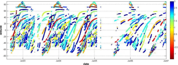
Figure 1 Location of GOMOS nighttime occultations of stars with effective temperature ≥6000 K used
in the analysis. Color indicates the stellar magnitude: the smaller magnitude, the brighter star.
Fig. 1. Location of GOMOS nighttime occultations of stars with effective temperature ≥6000 K used in the analysis. Color indicates the
stellar magnitude: the smaller magnitude, the brighter star.
which have a very good vertical resolution and accuracy (see Sect. 2), have confirmed the magnitude of the tertiary ozone maximum of 2–4 ppmv (Sofieva et al., 2004b).
Hartogh et al. (2004) pointed out that the distribution of odd oxygen during polar night conditions depends essen-tially on the complex history before the polar night started, on vertical transport from the thermosphere and on horizon-tal transport from the domain outside the polar night area. By using the combined dynamical and chemical transport model COMMA-IAP, the authors obtained a tertiary ozone mixing ratio close to the observations by the ground-based millime-ter radiomemillime-ter at ALOMAR, and presented detailed spatio-temporal distributions of mesospheric ozone.
To our knowledge, a description of the mean structure and seasonal variability of the observed tertiary ozone maximum has not been published thus far. In this paper, we present the first spatio-temporal distributions of tertiary ozone max-imum obtained from ozone measurements by GOMOS. We compare the experimental TOM distributions with that sim-ulated by the WACCM model. We discuss the influence of dynamics and energetic particle precipitation on variability of the tertiary ozone maximum.
2 Ozone measurements by GOMOS on Envisat
GOMOS (http://envisat.esa.int/instruments/gomos; Kyr¨ol¨a et al., 2004; Bertaux et al., 2004) on board the Envisat satellite is the first operational instrument that uses starlight for monitoring the atmospheric composition. The GOMOS spectrometers measure the stellar spectrum continuously as a star sets behind the Earth limb. Vertical profiles of ozone,
NO2, NO3, and aerosol extinction are retrieved from the
UV-Visible spectrometer measurements. Since the launch in
March 2002, GOMOS has performed more than 600 000 oc-cultations.
The basis for the geophysical data retrieval from GO-MOS measurements is the transmission spectra, which are obtained by dividing the spectra measured at different tan-gent altitudes by the reference spectrum measured above the atmosphere. In the GOMOS data processing, the inversion is split into two parts: the spectral inversion part and the vertical inversion part (Kyr¨ol¨a et al., 1993). In the spectral inversion, horizontal column densities are retrieved from the atmospheric transmission data from which refractive effects and scintillation have been removed. In the vertical inver-sion, vertical profiles are reconstructed from the horizontal column densities. The inversion is stabilized by Tikhonov-type regularization according to the target resolution (Sofieva et al., 2004a; Tamminen et al., 2004), which makes the ver-tical resolution pracver-tically independent of angles between the orbital plane and the direction to the star. In the mid-dle and upper mesosphere, the vertical resolution (including the smoothing properties of the inversion) of GOMOS ozone profiles is about 3 km.
For ozone, the valid altitude range is ∼10–100 km. The accuracy of the retrieval depends on stellar magnitude and spectral class. Only occultations of hot stars, which emit suf-ficiently at ultraviolet wavelengths, are able to provide infor-mation about ozone in the mesosphere and the thermosphere (Kyr¨ol¨a et al., 2006). For the analysis of the tertiary ozone maximum, we selected dark limb occultations (solar zenith
angle ≥107◦at the tangent point, and ≥90◦at the satellite) of
stars with effective temperature ≥ 6000 K. The accuracy of individual selected profiles at ∼70 km is ∼1.5-7%, depend-ing on stellar brightness.
In our analysis, we used GOMOS ozone data from 2002–2006. The spatio-temporal coverage of the selected
V. F. Sofieva et al.: Spatio-temporal observations of the tertiary ozone maximum 4441 nighttime GOMOS observations (131 500 occultations) is
shown in Fig. 1. It is characterized by a good coverage of winter poles, while summer poles are not covered due to the absence of dark limb conditions. During May–June 2003 and February–July 2005, GOMOS suffered from a pointing system malfunction, thus data are missing in these periods. Reduced azimuth angle range since August 2005 results in a decreased amount of GOMOS data since that time. The successive occultations of each star are nearly uniformly dis-tributed in the longitudinal direction (maximum 14 occulta-tions per day), and they are carried out approximately at the same local time. Therefore, being averaged over longitude, GOMOS measurements are a good representation of zonal mean data.
GOMOS data are very convenient for interannual com-parisons because occultations of the same stars are carried out approximately at the same locations and time in dif-ferent years. Ozone number density is retrieved from GO-MOS measurements. For calculation of mixing ratio, we used combined air density profiles based on ECMWF data in the stratosphere and on MSIS90 model (Hedin, 1990) in the mesosphere, at occultation locations. A procedure that ensures validity of the hydrostatic equation for the resulting profiles was applied.
3 Brief description of the WACCM model
The Whole Atmosphere Community Climate Model
(WACCM) was developed under the leadership of the National Center for Atmospheric Research (NCAR) for in-vestigation of interactions over the depth of the atmosphere. WACCM is a global model that extends from the ground
to 4.5×10⁻⁶hPa, approximately 145 km. The model is an
extension of the Community Atmosphere Model and uses the physical parameterizations from it (see Collins et al., 2004). The dynamical core of WACCM is based on the finite volume method of Lin (2004). The model includes fully interactive chemistry with 51 neutral species, 5 ions and electrons. It incorporates most of the physical and chemical mechanisms believed to be important for determining the dynamical and chemical structure of the middle atmosphere,
including the mesosphere and lower thermosphere.
Ex-tensions to physics include parameterizations of electron precipitation in the auroral oval, non-orographic gravity wave drag and molecular diffusion. A full description of the model dynamics, chemistry, radiation, and physical parameterizations is given in (Garcia et al. 2007) and (Marsh et al. 2007).
The WACCM simulations were carried out at 4◦×5◦
(lat-itude × long(lat-itude) resolution. The results of three ensemble simulations described in (Garcia et al., 2007) are used for the analysis presented in this paper; we present the mean distri-butions over the three ensemble realizations.
13
Jan03 Jan04 Jan05 Jan06
−80 −60 −40 −20 0 20 40 60 80 date latitude
Jan03 Jan04 Jan05 Jan06
−80 −60 −40 −20 0 20 40 60 80 date latitude 0.5 1 1.5 2 2.5 3 GOMOS WACCM
ozone mixing ratio (ppmv)
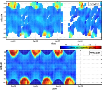
Figure 2 Ozone mixing ratio at 72 km. Top: from GOMOS measurements (zonal mean), bottom: from WACCM simulations (mean over three ensemble simulations for 0° longitude, midnight). Temporal and latitudinal averaging is nearly the same for the both experimental and model data.
Fig. 2. Ozone mixing ratio at 72 km. Top: from GOMOS
mea-surements (zonal mean), bottom: from WACCM simulations (mean over three ensemble simulations for 0◦longitude, midnight). Tem-poral and latitudinal averaging is nearly the same for the both ex-perimental and model data.
4 Spatio-temporal distributions of tertiary ozone maxi-mum
The explanation for the tertiary ozone maximum is that it
occurs as a result of Oxloss by catalytic cycles of OH and
HO2 that is decreasing because HOx production from
pho-tolysis of water vapor decreases with reducing UV radia-tion at high latitudes in winter (Marsh et al., 2001; Hartogh et al., 2004). Thus, the maximum mixing ratio should be achieved close to the polar night terminator. Figure 2 (top) shows ozone mixing ratio at 72 km obtained from the GO-MOS data in the period September 2002–December 2006. To produce the GOMOS distribution, data were first
aver-aged in 5◦×10 days (latitude × time) bins, and then
three-point smoothing (both in latitude and time) was applied to the data field. Although the maximum mixing ratio is achieved close to the polar night terminator (as predicted by the the-ory), the tertiary ozone maximum is observed also at very high latitudes, not only in the beginning and at the end, but also in the middle of winter (which was not predicted by the modelling results presented in (Hartogh et al., 2004, Fig. 11 therein). However, WACCM reproduces very well the evo-lution of the latitudinal distribution of ozone mixing ratio at
∼72 km (Fig. 2, bottom), including also specific features of
this distribution (temporal and latitudinal averaging is nearly the same for both experimental and model distributions). The only difference in these distributions is that WACCM pre-dicts slightly larger ozone mixing ratios (up to 5 ppmv) than that observed by GOMOS (not exceeding 4 ppmv).
4442 V. F. Sofieva et al.: Spatio-temporal observations of the tertiary ozone maximum 14 latitude altitude, km 2002−2003 −40 −20 0 20 40 60 80 45 50 55 60 65 70 75 80 85 90 latitude altitude, km 2003−2004 −40 −20 0 20 40 60 80 45 50 55 60 65 70 75 80 85 90 0.2 0.4 0.6 0.8 1 1.2 1.4 1.6 1.8 2 2.2 2.4 2.6 2.8 3 3.2 3.4 3.6 latitude altitude, km 2004−2005 −40 −20 0 20 40 60 80 45 50 55 60 65 70 75 80 85 90 latitude altitude, km 2005−2006
ozone mixing ratio (ppmv)
−40 −20 0 20 40 60 80 45 50 55 60 65 70 75 80 85 90
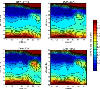
Figure 3 Latitude-altitude section of GOMOS ozone mixing ratio distribution (ppmv) in the longitudinal band from 30°W to 30° E averaged for the period 15 Dec - 15 Jan. Fig. 3. Latitude-altitude section of GOMOS ozone mixing ratiodistribution (ppmv) in the longitudinal band from 30◦W to 30◦E
averaged for the period 15 December–15 January.
Figure 3 shows altitude-latitude dependence of GOMOS
ozone mixing ratios in the longitudinal band from 30◦W to
30◦E averaged over the period 15 December–15 January, for
four NH winters. The latitudinal grid used in Fig. 3 is not uni-form; it is spaced according to data availability (see Fig. 1).
At high latitudes, the width of latitudinal bins is 5◦. The
peak mixing ratio is located at altitudes 65–75 km, and usu-ally its latitudinal position is close to the polar night termi-nator. Unlike the modelling results by Hartogh et al. (2004), the tertiary ozone maximum is not clearly isolated from the high latitudes as predicted by Fig. 9 in (Hartogh et al., 2004). In addition, Hartogh et al. (2004) predict large ozone values around the pole at upper altitudes (down to 75 km) indicat-ing strong downward transport of atomic oxygen from the thermosphere, which is not confirmed by the GOMOS data.
Figure 4 shows the analogous latitude-altitude sections ob-tained from WACCM simulations. The midnight model data
for 0◦ were averaged over three ensemble simulations and
over the same time period 15 December–15 January, as the GOMOS data. The distributions look similar, but the model ozone mixing ratios are ∼50% higher than in the GOMOS data. As seen in Fig. 3, ozone mixing ratios exhibit rather large variations from year to year. Since WACCM is a free-running climate model, the winds generated within the model are unlikely to match the observed winds on any one day. This difference in meteorology could contribute to the ap-parent discrepancy between model and observations. The overestimate of the magnitude of the TOM by WACCM is significantly smaller than it has been seen in the ROSE model (Marsh et al., 2001). Since this phenomenon involves hydro-gen chemistry and occurs only at high solar zenith angles,
15 latitude altitude, km 2002−2003 −40 −20 0 20 40 60 80 45 50 55 60 65 70 75 80 85 90 latitude altitude, km 2003−2004 −40 −20 0 20 40 60 80 45 50 55 60 65 70 75 80 85 90 latitude altitude, km 2004−2005
ozone mixing ratio (ppmv)
−40 −20 0 20 40 60 80 45 50 55 60 65 70 75 80 85 90 0.2 0.4 0.6 0.8 1 1.2 1.4 1.6 1.8 2 2.2 2.4 2.6 2.8 3 3.2 3.4 3.6
Figure 4 Altitude-latitude sections from WACCM simulations. The data for midnight at longitude 0° are averaged over the period from 15 December to 15 January and over three ensemble simulations.
Fig. 4. Altitude-latitude sections from WACCM simulations. The
data for midnight at longitude 0◦are averaged over the period from 15 December to 15 January and over three ensemble simulations.
it suggests that the model overestimates could stem from in-accuracies in the simulated water distribution in the winter mesosphere or problems with the photolysis rate of water at near-polar night conditions.
According to Figs. 3 and 4, the tertiary ozone maximum can extend to the pole. This extension varies from year to year. It seems that the appearance of the tertiary ozone maxi-mum close to the pole is related to the intensity of horizontal mixing at high latitudes (see also below).
It is interesting that the altitude position of the tertiary ozone maximum shifts downward on moving closer to the pole. This might be related to the downward transport in the polar night area and could illustrate the peculiarities of the meridional circulation.
5 Dynamical aspects
In order to follow the evolution of tertiary ozone during
po-lar night, we selected two latitudinal bands in the NH: 70◦–
76◦N and 80◦–90◦N. These latitudinal bands have a very
good daily coverage by occultations of the brightest stars (Sirius, Rigel, Procyon), which allow very accurate ozone measurements (uncertainty of individual profiles is ∼1.5–2% at altitudes ∼70 km).
The time series of ozone mixing ratio in the mesosphere in two latitudinal bands, for four Northern Hemisphere win-ters are shown in Fig. 5. Based on the modelling results by Hartogh et al. (2004, Figs. 5 and 6), one would expect that the seasonal variations of the tertiary ozone maximum at these latitudes to consist of two isolated peaks in the begin-ning (October-November) and at the end (February–March)
V. F. Sofieva et al.: Spatio-temporal observations of the tertiary ozone maximum 4443
16
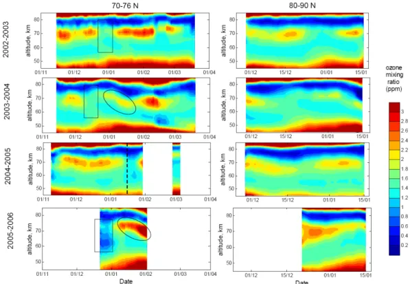
Figure 5 Time series of zonal mean ozone mixing ratio profiles are shown for two latitudinal bands: 70°-76° N (left) and 80°-90° N (right). 5-day average data are presented. Rectangles indicate periods of sudden stratospheric warmings. Ovals indicate strong downward transport. The dashed line in the subplot for the winter 2004-2005 indicates the onset of SPE in January 2005.
Fig. 5. Time series of zonal mean ozone mixing ratio profiles are shown for two latitudinal bands: 70◦-76◦N (left) and 80◦–90◦N (right). 5-day average data are presented. Rectangles indicate periods of sudden stratospheric warmings. Ovals indicate strong downward transport. The dashed line in the subplot for the winter 2004-2005 indicates the onset of SPE in January 2005.
of winter, according to the variation of the polar night termi-nator. However, the seasonal variations of ozone mixing ratio in Fig. 5 do not show such behavior. As seen in Fig. 5, the tertiary ozone maximum is observed usually throughout the winter, but its magnitude is subject to significant variations.
During sudden stratospheric warmings, the tertiary ozone mixing ratio can decrease significantly, as during the ma-jor stratospheric warming in December 2003 (Manney et al., 2005), or the tertiary ozone maximum can even be com-pletely destroyed, as during the stratospheric warming in late January 2006, as seen in Fig. 5. Due to a long lifetime of ozone in polar night conditions, the downward transport of the polar air by the meridional circulation can be observed in the tertiary ozone time series. In particular, two very strong downward transport events – in January 2004 discussed by Hauchecorne et al. (2007) and in February-March 2006 dis-cussed by Randall et al. (2006) – are clearly observed in Fig. 5. It is interesting that strong downward transport is observed after sudden stratospheric warmings.
Comparing Fig. 5 and Fig. 3, one might suggest that there exists a relationship between the isolation of the tertiary ozone maximum from the pole and intensity of downward transport. Since the data shown in Fig. 3 are averaged over the period 15 December–15 January, only one subplot in Fig. 3, for winter 2003–2004, includes the period of strong downward transport. The tertiary ozone maximum is more
isolated from the pole for 2003–2004 than for other years. It seems that cases with strong downward transport also have a decrease in horizontal mixing, thus resulting in a better iso-lation of tertiary ozone maximum from the pole, and vice versa.
6 Influence of energetic particles precipitation
Energetic particle precipitation events, such as Solar Proton
Events (SPE), produce HOx in the high latitude middle
at-mosphere, including the polar night terminator region where the tertiary ozone maximum is formed. Increased ionization
caused by particle precipitation leads to HOxproduction via
ion chemical reactions (e.g., Solomon et al., 1981).
Theoret-ical predictions of significant HOx production and the
sub-sequent ozone loss have been verified by the observations of MLS/Aura and GOMOS/Envisat instruments (Verronen et
al., 2006). In the terminator area the HOxconcentration is
relatively low, therefore moderate SPE production can
com-pensate for the reduced natural HOx production in the
ter-minator area and can even exceed it. Sepp¨al¨a et al. (2006) have shown that the tertiary ozone maximum disappeared during the January 2005 SPE. Figure 6 presents another ex-ample/confirmation of TOM sensitivity to particle forcing, the destruction of TOM by the moderate SPE of December
4444 V. F. Sofieva et al.: Spatio-temporal observations of the tertiary ozone maximum
17 Figure 6 Top: daily ozone mixing ratio profiles at latitudes 60°-90°N in December 2006. Bottom: proton flux measured by GOES-11. Note the destruction of tertiary ozone maximum caused by the SPE. Envisat data are unavailable for 13-15 December 2006, due to an anomaly that was probably the result of high geomagnetic activity.
Fig. 6. Top: daily ozone mixing ratio profiles at latitudes 60◦–90◦N in December 2006. Bottom: proton flux measured by GOES-11. Note the destruction of tertiary ozone maximum caused by the SPE. Envisat data are unavailable for 13–15 December 2006, due to an anomaly that was probably the result of high geomagnetic activity.
2006. Larger values ∼2 ppmv are seen at 65–70 km until 7 December when the SPE began. After the onset of the SPE, the ozone mixing ratio drops below 0.5 ppmv. The data show TOM recovery on 16 December when the SPE particle forc-ing declines to the quiet-time level. Because of the short
pho-tochemical lifetime of HOx, low ozone values are observed
only when the particle fluxes are elevated. As the forcing
stops, the HOx production also stops and the HOxamount
returns to the normal level within a day, thus resulting in ozone recovery. SPEs cause pronounced changes in TOM, but they are sporadic and typically last only for several days. Electron precipitation in the auroral oval region also affects TOM. Electron precipitation is more continuous but of lower intensity compared to SPE. For example, in Fig. 5 the largest ozone mixing ratios are observed in January–February 2006 when energetic particle forcing was lowest in 2002–2006 as indicated by geomagnetic activity indices (Sepp¨al¨a et al., 2007). This indicates the importance of including particle precipitation in models in order to obtain quantitative agree-ment with measureagree-ments in the mesosphere.
7 Summary
In this paper, we show the first experimental global distri-bution and seasonal variations of the tertiary ozone maxi-mum in 2002–2006, as obtained from GOMOS data. The tertiary ozone maximum is observed at high latitudes in win-ter. Peak ozone mixing ratio is from 2 to 4 ppmv, and it can be observed at altitudes 65–75 km, depending on latitude and time. The obtained distributions can be used for validation of global circulation and chemical transport models.
The WACCM model predicts well the position of the ter-tiary ozone maximum and its latitudinal extent, thus confirm-ing general understandconfirm-ing of the processes related to the for-mation of the tertiary ozone maximum. Peak concentrations are slightly overestimated in WACCM compared to GOMOS data. Differences in the model and experimental meteorolog-ical fields, inaccuracies in the simulated water distribution in the winter mesosphere or problems with the photolysis rate of water at near-polar night conditions might contribute to the observed discrepancy.
Energetic particle precipitation significantly affects the ozone concentrations at the location of the tertiary maximum (and in the mesosphere in general). Even moderate SPEs can destroy the tertiary ozone maximum. TOM mixing ratios are higher during periods of low energetic particle (electron
V. F. Sofieva et al.: Spatio-temporal observations of the tertiary ozone maximum 4445 and proton) precipitation, as was observed in the Northern
Hemisphere in Jan-Feb 2006. This indicates the importance of including energetic particle precipitation in models of the middle atmosphere.
Acknowledgements. The work of VS, PV and AS was supported by
the Academy of Finland (postdoctoral research projects of VS and AS, THERMES project). The National Center for Atmospheric Re-search is operated by the University Corporation for Atmospheric Research under sponsorship of the National Science Foundation.
Edited by: P. Bernath
References
Bertaux, J. L., Hauchecorne, A., Dalaudier, F., Cot, C., Kyrola, E., Fussen, D., Tamminen, J., Leppelmeier, G. W., Sofieva, V., Has-sinen, S., Fanton d’Andon, O., Barrot, G., Mangin, A., Theodore, B. Guirlet, M. Korablev, O., Snoeij, P. Koopman, R., and Fraisse, R.: First results on GOMOS/Envisat, Adv. Space Res., 33, 1029– 1035, doi:10.1016/j.asr.2003.09.037, 2004.
Collins, W. D., Rasch, P. J., Boville, B. A., Hack, J. J., McCaa, J. R., Williamson, D. L., Kiehl, J. T., and Briegleb, B.: Description of the NCAR Community Atmosphere Model (CAM 3.0), Natl. Cent. for Atmos. Res., Boulder, Colorado, USA, 2004.
Garcia, R. R., Marsh, D. R., Kinnison, D. E., Boville, B. A., and Sassi, F.: Simulation of secular trends in the mid-dle atmosphere, 1950–2003, J. Geophys. Res., 112, D09301, doi:10.1029/2006JD007485, 2007
Grenfell J. L., Lehmann, R., Mieth, P., Langematz, U., and Steil, B.: Chemical reaction pathways affecting stratospheric and mesospheric ozone, J. Geophys. Res., 111, D17311, doi:10.1029/2004JD005713, 2006.
Hartogh, P., Jarchow, C., Sonnemann, G. R., and Gry-galashvyly, M.: On the spatiotemporal behavior of ozone within the upper mesosphere/mesopause region under nearly polar night conditions, J. Geophys. Res., 109, D18303, doi:10.1029/2004JD004576, 2004.
Hauchecorne, A., Bertaux, J.-L., Dalaudier, F., Russell III, J. M., Mlynczak, M. G., Kyr¨ol¨a, E., and Fussen, D.: Large increase of NO2 in the north polar mesosphere in January–February 2004: Evidence of a dynamical origin from GOMOS/ENVISAT and SABER/TIMED data, Geophys. Res. Lett., 34, L03810, doi:10.1029/2006GL027628, 2007.
Hedin, A. E.: Extension of the MSIS Thermosphere Model into the Middle and Lower Atmosphere, J. Geophys. Res., 96(A2), 1159–1172, 1991.
Kyr¨ol¨a, E., Sihvola, E., Kotivuori, Y., Tikka, M., Tuomi, T., and Haario, H.: Inverse theory for occultation measurements. 1. Spectral inversion, J. Geophys. Res., 98(D4), 7367–7381, 1993. Kyr¨ol¨a, E., Tamminen, J., Leppelmeier, G. W., Sofieva, V.,
Has-sinen, S., Bertaux, J. L., Hauchecorne, A., Dalaudier, F., Cot, C., Korablev, O., Fanton d’Andon, O., Barrot, G., Mangin, A., Theodore, B., Guirlet, M., Etanchaud, F., Snoeij, P., Koopman, R., Saavedra, L., Fraisse, R., Fussen, D., and Vanhellemont, F.: GOMOS on Envisat: An overview, Adv. Space Res., 33, 1020– 1028, doi:10.1016/S0273-1177(03)00590-8, 2004.
Kyr¨ol¨a E., Tamminen, J., Leppelmeier, G. W., Sofieva, V., Hassi-nen, S., Sepp¨al¨a, A., VerroHassi-nen, P. T., Bertaux, J. L., Hauchecorne, A., Dalaudier, F., Fussen, D., Vanhellemont, F., Fanton d’Andon, O., Barrot, G., Mangin, A., Theodore, B., Guirlet, M., Koop-man, R., Saavedra de Miguel, L., Snoeij, P., Fehr, T., Mei-jer, Y., and Fraisse, R.: Nighttime ozone profiles in the strato-sphere and mesostrato-sphere by the Global Ozone Monitoring by Oc-cultation of Stars on Envisat, J. Geophys. Res., 111, D24306, doi:10.1029/2006JD007193, 2006.
Lin, S.-J.: A vertically Lagrangian finite-volume dynamical core for global models, Mon. Weather Rev., 132, 2293–2307, 2004. Manney, G. L., Kr¨uger, K., Sabutis, J. L., Sena, S. A., and Pawson,
S.: The remarkable 2003– 2004 winter and other recent warm winters in the Arctic stratosphere since the late 1990s, J. Geo-phys. Res., 110, D04107, doi:10.1029/2004JD005367, 2005. Marsh, D., Smith, A., Brasseur, G., Kaufmann, M., and
Gross-mann, K.: The existence of a tertiary ozone maximum in the high-latitude middle mesosphere, Geophys. Res. Lett., 28(24), 4531–4534, 2001
Marsh, D. R., Garcia, R. R., Kinnison, D. E., Boville, B. A., Sassi, F., Solomon, S. C., and Matthes, K.: Modeling the whole atmosphere response to solar cycle changes in radia-tive and geomagnetic forcing, J. Geophys. Res., 112, D23306, doi:10.1029/2006JD008306, 2007.
Randall, C. E., Harvey, V. L., Singleton, C. S., Bernath, P. F., Boone, C. D., and Kozyra, J. U.: Enhanced NOxin 2006 linked to
up-per stratospheric Arctic vortex, Geophys. Res. Lett., 33, L18811, doi:10.1029/2006GL027160, 2006.
Sepp¨al¨a, A., Verronen, P. T., Sofieva, V. F., Tamminen, J., Kyrola, E., Rodger, C. J., and Clilverd, M. A.: Destruction of the Tertiary Ozone Maximum During a Solar Proton Event, Geophys. Res. Lett., 33, L07804, doi:10.1029/2005GL025571, 2006.
Sepp¨al¨a, A., Verronen, P. T., Clilverd, M. A., Randall, C. E., Tamminen, J., Sofieva, V., Backman, L., and Kyr¨ol¨a, E.: Arc-tic and AntarcArc-tic polar winter NOx and energetic particle
pre-cipitation in 2002–2006, Geophys. Res. Lett., 34, L12810, doi:10.1029/2007GL029733, 2007.
Sofieva, V. F., Tamminen, J., Haario, H., Kyr¨ol¨a, E., and Lehtinen, M.: Ozone profile smoothness as a priori information in the in-version of limb measurements, Ann. Geophys., 22(10), 3411–34, 2004a.
Sofieva, V. F., Verronen, P. T., Kyr¨ol¨a, E., Hassinen, S., and GO-MOS CAL/VAL team: The tertiary ozone maximum in the mid-dle mesosphere as seen by GOMOS on Envisat; Quadrennial Ozone Symposium, 2004b.
Solomon, S., Rusch, D. W., G´erard, J.-C., Reid, G. C., and Crutzen, P. J.: The effect of particle precipitation events on the neutral and ion chemistry of the middle atmosphere: II. Odd hydrogen, Planet. Space Sci., 8, 885–893, 1981.
Tamminen J., Kyr¨ol¨a, E., and Sofieva, V.: Does a priori information improve occultation measurements? in Occultations for Probing Atmosphere and Climate, edited by: Kirchengast, G., Foelshe, U., and Steiner, A., Springer Verlag, 87–98, 2004
Verronen, P. T., Sepp¨al¨a, A., Kyr¨ol¨a, E., Tamminen, J., Pickett, H. M., and Turunen, E.: Production of odd hydrogen in the meso-sphere during the January 2005 solar proton event, Geophys. Res. Lett., 33, L24811, doi:10.1029/2006GL028115, 2006.