The effect of ocean mixed layer depth on
climate in slab ocean aquaplanet experiments
The MIT Faculty has made this article openly available.
Please share
how this access benefits you. Your story matters.
Citation
Donohoe, Aaron, Dargan M. W. Frierson, and David S. Battisti.
“The Effect of Ocean Mixed Layer Depth on Climate in Slab Ocean
Aquaplanet Experiments.” Climate Dynamics 43.3–4 (2014): 1041–
1055.
As Published
http://dx.doi.org/10.1007/s00382-013-1843-4
Publisher
Springer Berlin Heidelberg
Version
Author's final manuscript
Citable link
http://hdl.handle.net/1721.1/103412
Terms of Use
Article is made available in accordance with the publisher's
policy and may be subject to US copyright law. Please refer to the
publisher's site for terms of use.
Climate Dynamics manuscript No. (will be inserted by the editor)
The effect of ocean mixed layer depth on climate in slab
1
ocean aquaplanet experiments.
2
Aaron Donohoe · Dargan M.W. Frierson · 3
David S. Battisti 4
5
Manuscript submitted June 10, 2013
6
Abstract 7
The effect of ocean mixed layer depth on climate is explored in a suite of 8
slab ocean aquaplanet simulations with different mixed layer depths ranging 9
from a globally uniform value of 50 meters to 2.4 meters. In addition to the 10
expected increase in the amplitude of the seasonal cycle in temperature with 11
decreasing ocean mixed layer depth, the simulated climates differ in several 12
less intuitive ways including fundamental changes in the annual mean climate. 13
The phase of seasonal cycle in temperature differs non-monotonically with 14
increasing ocean mixed layer depth, reaching a maximum in the 12 meter 15
slab depth simulation. This result is a consequence of the change in the source 16
of the seasonal heating of the atmosphere across the suite of simulations. In 17
the shallow ocean runs, the seasonal heating of the atmosphere is dominated 18
by the surface energy fluxes whereas the seasonal heating is dominated by 19
direct shortwave absorption within the atmospheric column in the deep ocean 20
runs. The surface fluxes are increasingly lagged with respect to the insolation 21
as the ocean deepens which accounts for the increase in phase lag from the 22
shallow to mid-depth runs. The direct shortwave absorption is in phase with 23
insolation, and thus the total heating comes back in phase with the insolation 24
as the ocean deepens more and the direct shortwave absorption dominates the 25
seasonal heating of the atmosphere. 26
The intertropical convergence zone (ITCZ) follows the seasonally vary-27
ing insolation and maximum sea surface temperatures into the summer hemi-28
sphere in the shallow ocean runs whereas it stays fairly close to the equator 29
in the deep ocean runs. As a consequence, the tropical precipitation and re-30
gion of high planetary albedo is spread more broadly across the low latitudes 31
Aaron Donohoe
Dept. of Earth, Atmospheric and Planetary Sciences, Room Number 54-918, 77 Massachusetts Avenue, Cambridge, MA 02139-4307. E-mail: thedhoe@mit.edu
D.M.W. Frierson · D.S. Battisti
in the shallow runs, resulting in an apparent expansion of the tropics relative 32
to the deep ocean runs. As a result, the global and annual mean planetary 33
albedo is substantially (20%) higher in the shallow ocean simulations which 34
results in a colder (7C) global and annual mean surface temperature. The in-35
creased tropical planetary albedo in the shallow ocean simulations also results 36
in a decreased equator-to-pole gradient in absorbed shortwave radiation and 37
drives a severely reduced (≈ 50%) meridional energy transport relative to the 38
deep ocean runs. As a result, the atmospheric eddies are weakened and shifted 39
poleward (away from the high albedo tropics) and the eddy driven jet is also 40
reduced and shifted poleward by 15◦relative to the deep ocean run.
41
Keywords seasonal cycle · aquaplanet · expansion of tropics 42
1. Introduction 43
The seasonal cycle of temperature in the extratropics is driven by seasonal variations 44
in insolation that are comparable in magnitude to the annual mean insolation. The 45
majority of the seasonal variations in insolation are absorbed in the ocean Fasullo 46
and Trenberth (2008a,b), which has a much larger heat capacity than the overlying 47
atmosphere. This energy never enters the atmospheric column to drive seasonal vari-48
ations in atmospheric temperature and circulation. The heat capacity of the ocean 49
plays a fundamental role in setting both the magnitude and phasing of the seasonal 50
cycle in the atmosphere. The Earth’s climate would be fundamentally different if the 51
ocean’s heat capacity was not substantially larger than that of the atmosphere. 52
In a forced system with a heat capacity and negative feedbacks (damping), the 53
phase lag of the response increases with increasing heat capacity, reaching quadra-54
ture phase with the forcing in the limit of very large heat capacity (Schneider 1996). 55
Therefore, in the extratropical climate system– where the insolation is the forcing and 56
the Planck feedback and dynamic energy fluxes are the dominant negative feedbacks– 57
one would expect that the phase lag of temperature with respect to insolation would 58
increase with increasing ocean heat capacity. We will demonstrate that this expecta-59
tion is not realized in a set of experiments with an idealized climate model; the phase 60
lag of atmospheric temperature is a non-monotonic function of ocean heat capacity. 61
We argue that increasing ocean heat capacity moves the system from a regime in 62
which the seasonal heating of the atmosphere is dominated by the energy fluxes from 63
the surface (ocean) to the atmosphere to a regime where the heating is dominated by 64
the sun heating the atmosphere directly via shortwave absorption in the atmospheric 65
column. In the latter regime, the surface and atmospheric energy budgets are partially 66
decoupled and the atmospheric heating is nearly in phase with the insolation result-67
ing in a small phase lag of the seasonal temperature response. Recently, Donohoe 68
and Battisti (2013) demonstrated that the seasonal heating of the atmosphere in the 69
observations is dominated by direct shortwave absorption in the atmospheric column 70
as opposed to surface energy fluxes, which is akin to the large ocean heat capacity 71
regime discussed above. 72
The heat capacity of the climate system does not contribute to the annual mean 73
energy budget in the theory of energy balance models (North 1975) because there 74
is no heat storage in equilbruim. However, the magnitude of the seasonal cycle can 75
impact the annual mean energy budget through the rectification of non-linearities 76
and/or the covariance of processes acting over the seasonal cycle (i.e. the correlation 77
between seasonal anomalies in insolation and albedo). Therefore, the ocean heat ca-78
pacity may impact the annual mean climate. Indeed, we demonstrate here that the 79
ocean heat capacity has a large impact on the modeled climate system in the annual 80
mean including the global mean temperature, the global energy budget, the extent 81
of the tropics, the meridional energy transport, and the location and intensity of the 82
surface westerlies. 83
Slab ocean models are widely used to assess the equilibrium climate sensitivity 84
in global climate models (Danabasoglu and Gent 2009) because the system comes to 85
equilibrium rapidly as compared to the full-depth ocean model. Slab ocean models 86
are also widely used in idealized simulations (Kang et al. 2008; Rose and Ferreira 87
2013) to model the response of the climate system to prescribed anomalies in ocean 88
heat transport. The sensitivity of climate to mixed layer depth in these simulations is 89
often neglected. 90
In this study, we analyze the effect of slab ocean depth on climate (temperature, 91
precipitation, winds, and energy fluxes) in a suite of aquaplanet slab ocean experi-92
ments, each with a different, globally uniform ocean mixed layer depth. This paper 93
is organized as follows. In Section 2, we introduce the models and observational data 94
sets we will compare the models to. We then analyze the amplitude and phase of 95
the seasonal cycle of atmospheric temperature and interpret these results in terms 96
of the source of the seasonal heating of the atmosphere (Section 3). In Section 4, 97
we analyze the seasonal migration of the inter-tropical convergence zone (ITCZ) in 98
the slab-ocean aquaplanet simulations and its impact on the tropical precipitation . 99
We also demonstrate in this section that the seasonal migration of the ITCZ causes 100
a large residual contribution to the global and annual average planetary albedo and, 101
hence, the global energy budget and global mean temperature. Lastly, in Section 5, 102
we demonstrate that the amplitude of the seasonal cycle also modifies the meridional 103
heat transport in the climate system by way of modifying the meridional structure of 104
planetary albedo. As a consequence, both the magnitude and location of the jets, in-105
cluding the surface westerlies, change as the amplitude of the seasonal cycle changes. 106
A summary and discussion follows in Section 6. 107
2. Data and methods 108
We will analyze the effect of ocean heat capacity on climate in a suite of slab-ocean 109
aquaplanet simulations with different ocean mixed layer depths. Here we describe 110
the model runs used. The analysis of the model output will then be compared to 111
observations to put the results in context. We also describe the observational data 112
sources in this section. 113
2a. Slab-ocean aquaplanet simulations 114
We couple an atmospheric general circulation model to a uniform constant depth slab 115
ocean that covers the entire globe – hereafter an aquaplanet. We perform five experi-116
ments with prescribed ocean depths of 2.4, 6, 12, 24, and 50 meters. The heat capacity 117
of the 2.4 m slab ocean is equivalent to that of the atmosphere while the heat capacity 118
in the 50 m run is more than 20 times that of the atmosphere. There is no Q flux to 119
the ocean; the ocean does not transport energy. Sea ice is prohibited from forming 120
in the model, even if the sea-surface temperature is below the freezing point of sea 121
water. The atmospheric model is the Geophysical Fluid Dynamics Lab Atmospheric 122
Model version 2.1 (Delworth et al. 2006) featuring a finite volume dynamical core 123
(Lin 2004) with a horizontal resolution of approximately 2◦latitude, 2.5◦longitude
124
and 24 vertical levels. The model is forced by seasonally varying solar insolation with 125
zero eccentricity and 23.439◦obliquity. The model is run for twenty years and the
126
model climatology is taken from the last five years of the integrations; these choices 127
ensure the model is spun up and the seasonal cycle is adequately sampled. 128
The atmospheric energy budget is 129
dE
dt = SWABS + SHF − OLR − ∇ · (U MSE) , (1)
where E is the column integral of sensible and latent heat (CpT +Lq), OLR is the 130
outgoing longwave radiation, MSE is the moist static energy (CpT +Lq + gZ), and 131
the term on the right represents the atmospheric energy flux convergence integrated 132
over the column of the atmosphere. SWABS is the shortwave absorption within the 133
atmospheric column, and represents the sun directly heating the atmosphere: 134
SWABS= SW ↓T OA−SW ↑T OA+SW ↑SU RF −SW ↓SU RF . (2)
SHFis the net (turbulent plus longwave radiation) exchange of energy between the
135
surface and the atmosphere: 136
SHF= SENS ↑SU RF +LH ↑SU RF +LW ↑SU RF −LW ↓SU RF, (3)
where SENS is the sensible energy flux and LH is the latent energy flux, both defined 137
as positive upwards to the atmosphere. We note that SHF does not include solar fluxes 138
because the surface solar fluxes are an exchange of energy between the surface and 139
the sun and the solar impact on the atmospheric budget is accounted for in SWABS. 140
See (Donohoe and Battisti 2013) for further discussion. 141
We calculate SWABS and SHF from equations 2 and 3 respectively using the 142
model output of the fluxes at the top of the atmosphere (TOA) and the surface. dEdt,
143
hereafter the storage, is calculated from the finite difference of the monthly column 144
integrated temperature and specific humidity. The energy transport convergence is 145
calculated as the residual of equation 1. 146
2b. Observational data 147
We use the ERA-Interim Reanalysis climatological (1979-2010) atmospheric temper-148
ature data to define the amplitude and phase of the observed atmospheric temperature. 149
The radiative fluxes used are from the corrected long term climatologies (Fasullo and 150
Trenberth 2008a) of the Clouds and Earth’s Radiant Energy System (CERES) ex-151
periment (Wielicki et al. 1996). The atmospheric energy flux convergences are from 152
Donohoe and Battisti (2013) and are derived from ERA-Interim Reanalysis using the 153
advective form of the equations. SWABS is assessed directly from the climatological 154
averaged CERES data including the (AVG) surface shortwave fluxes. SHF is calcu-155
lated as a residual from equation 1. 156
3. The amplitude and phase of the seasonal cycle of atmospheric temperature 157
and the source of atmospheric heating 158
The seasonal amplitude of temperature, defined as the amplitude of the annual har-159
monic, in the slab-ocean aquaplanet simulations is shown in the left panel of figure 160
1. As expected, the seasonal amplitude decreases with increasing mixed layer depth 161
at both the surface (solid lines) and in the mid-troposphere (dashed line). In the shal-162
low mixed layer depth runs, the seasonal cycle of temperature is larger at the surface 163
then it is in the mid-troposphere. In contrast, the seasonal amplitude of temperature 164
is largest in the mid-troposphere for the deep mixed layer depth runs. The observed 165
amplitude of the seasonal cycle above the Southern Ocean (between 30◦S and 65◦S –
166
upper right panel of Figure 1) resembles that of the 50 meter run, with a small ampli-167
tude and amplified seasonal cycle aloft. Poleward of 65◦S the influence of the
Antarc-168
tic continent can be seen with a larger and surface amplified seasonal amplitude of 169
temperature. The seasonal amplitude in the Northern extratropics is comparable in 170
magnitude to the 12m run and shows the surface amplification seen in the shallow 171
mixed runs, reflecting the large and surface amplified seasonal cycle over the land 172
masses. 173
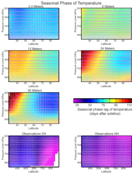
The phase lag of the tropospheric averaged (below 250 hPa) temperature rela-174
tive to the insolation varies non-monotonically with mixed layer depth (bottom panel 175
of Figure 1); the phase lag in the high-latitudes (poleward of 50◦) increases as the
176
mixed-layer depth increases from 2.4 meters to 12 meters but then decreases as the 177
mixed layer depth increases further from 12 meters to 50 meters. This behavior is not 178
expected from a system with a single heat capacity dictated by the ocean mixed-layer 179
depth. The observed seasonal cycle of temperature has a substantially smaller phase 180
lag than any of the aquaplanet simulations (lower right panel of Figure 1). The verti-181
cal structure of the phase of the seasonal cycle in temperature (Figure 2) shows that 182
the phase is nearly vertically uniform in the shallow mixed layer depth experiments, 183
suggesting that the entire column responds in unison to seasonal variations in inso-184
lation. In contrast, in the deep mixed layer runs, the temperature aloft leads that at 185
the surface by of order one month in the high latitudes1. The observed seasonal cycle
186
of temperature has a smaller phase lag than the aquaplanet simulations at all levels. 187
The observed temperature aloft leads that at the surface (akin to the deep mixed layer 188
depth runs) over the Southern Ocean whereas the phase is nearly vertical invariant 189
(akin to the shallow mixed layer depth runs) throughout the Northern extratropics 190
and over Antarctica. 191
1 We note that the seasonal cycle of temperature in the deep runs is delayed aloft in the vicinity of
40◦. This phase lag is a consequence of reduced eddy energy flux divergence during the warm season that
is driven by extratropical atmospheric heating leading which leads to a reduced meridional temperature gradient aloft during the late summer. This acts as a phase delayed source of heating in the subtropical troposphere which is driven non-locally.
We argue that the effect of ocean mixed layer depth on the amplitude, phase, and 192
vertical structure of the seasonal cycle in temperature can be understood by analyz-193
ing the source of the seasonal heating of the atmosphere. Specifically, the seasonal 194
heating of the atmosphere is dominated by the upward energy fluxes from the ocean 195
to the atmosphere (SHF) in the shallow mixed layer experiments whereas it is dom-196
inated by direct absorption of shortwave radiation (SWABS) in the deep mixed-layer 197
depth experiments. The time series of the seasonal heating (annual mean removed) 198
of the atmosphere by SWABS, SHF and their sum (total heating) averaged poleward 199
of 40◦N is shown in Figure 3. SWABS has a seasonal amplitude of order 50 W m−2,
200
is nearly in phase with the insolation and varies very little with mixed layer depth. 201
This result is consistent with water vapor and ozone in the atmosphere absorbing 202
approximately 20% of the insolation (Chou and Lee 1996) during all seasons. The 203
increased amplitude and phase lag of SWABS in the 2.4 meter runs is a consequence 204
of the moistening of the extratropical hemisphere during the late summer, resulting in 205
seasonal variations in the fraction of insolation absorbed in the column that peak in 206
late summer. We also note that the seasonal cycle of SWABS in the observations are 207
well replicated in the models suggesting that the basic state shortwave absorptivity is 208
well captured in the aquaplanet model. 209
In contrast to the nearly mixed-layer depth invariant SWABS, the seasonal cycle 210
of SHF decreases markedly with increasing mixed-layer depth while the phase lag 211
concurrently increases with increased mixed layer depth. In the limit of zero surface 212
heat capacity, we would expect the upward SHF to match the net shortwave radiation 213
at the surface because, there can be no storage in the surface. In the 2.4 meter run, 214
the seasonal amplitude of the SHF is 75 W m−2and is 62% of the amplitude of the
215
net shortwave radiation at the surface. The SHF lags the surface solar radiation by 29 216
days. Although the heat capacity of the ocean is non-negligble in the 2.4 meter run, 217
the majority of the surface shortwave radiation gets fluxed upward to the atmospheric 218
columnn with a small time lag2. In contrast, in the 50 meter run, the entirety of the
219
seasonal variations in surface shortwave radiation (not shown) are stored in the ocean 220
mixed-layer; the seasonal amplitude of energy storage in the extratropical ocean ex-221
ceeds the seasonal amplitude of net shortwave radiation at the surface (by 20%) as the 222
atmosphere fluxes energy to the ocean via downward a SHF during the warm season. 223
The latter flux is made possible by the fact that the atmosphere is being heated di-224
rectly by SWABS in the summer and losing energy via the interaction with the ocean 225
surface. This also explains why the seasonal cycle of temperature is amplified aloft in 226
the deep mixed layer depth runs (upper left panel of Figure 1) since the distribution of 227
SWABSis nearly invariant throughout the troposphere (Donohoe and Battisti 2013)
228
but the loss of energy to the ocean is confined to the boundary layer. 229
2 We note that, the seasonal amplitude of extratropical shortwave radiation absorbed at the surface is
in phase with the insolation but has 57% of the seasonal amplitude of the insolation (125 W m−2 as
compared to 220 W m−2) which represents the shortwave opacity of the atmosphere times the surface
co-albedo (0.92). Thus, in the limit of zero surface heat capacity we would expect that approximately 57% of the seasonal insolation to enter the atmospheric column via SHF as compared to the 20% of insolation absorbed directly in the atmospheric column (SWABS). In this case, there is an approximatley 3:1 heating ratio of SHF:SWABS, similar to the observed annual mean ratio (Donohoe and Battisti 2013).
The suite of aquaplanet mixed-layer experiments span two different regimes of 230
seasonal energy input into the atmosphere; the seasonal heating of the atmosphere is 231
dominated by the SHF in the shallow mixed layer runs while the seasonal heating of 232
the atmosphere is dominated by SWABS in the deep mixed layer runs (Figure 3). The 233
transition between the two regimes occurs for the 6 and 12 meter runs where both 234
SWABSand SHF contribute to the seasonal heating of the atmosphere. The phase
235
lag of SHF increases with increasing mixed layer depth as a consequence of the sea 236
surface temperatures lagging the insolation more as the thermal inertia of the system 237
increases. 238
The phase of the total heating varies non-monotonically with mixed layer depth 239
and can be understood in terms of the transition between a regime where seasonal 240
heating is dominated by SHF to one where SWABS dominates the seasonal heating 241
of the atmosphere. If the atmosphere was transparent to shortwave radiation (SWABS 242
= 0) then the phase lag of atmospheric temperature would increase monotonically 243
with increasing ocean mixed layer depth along with the phase of SHF. Indeed, as 244
the ocean mixed layer depth increases from 2.4m to 6m, the total seasonal heating of 245
the atmosphere becomes more phase lagged, reflecting the contribution SHF (Figure 246
3, bottom panel). However, the amplitude of SHF also decreases with increasing 247
mixed layer depth and the seasonal heating of the atmosphere becomes increasingly 248
dominated by SWABS; SWABS and SHF have nearly identical seasonal amplitudes in 249
the 6m run and the seasonal amplitude of SWABS exceeds that of SHF by a factor of 250
three in the 24m run. Because SWABS is nearly in phase with the insolation (and SHF 251
lags the insolation), the phase lag of total atmospheric heating decreases as the mixed 252
layer depth increases from 6m to 50m and the seasonal heating becomes dominated 253
by SWABS. In the 50m run, the seasonal flow of energy between the atmosphere and 254
the surface has completely reversed relative to the 2.4m run (and the annual mean): 255
the atmosphere is heated directly by the sun during the warm season and subsequently 256
fluxes energy downward to the ocean resulting in an amplified and phase leading 257
seasonal cycle aloft relative to the surface (Figure 1 and 2 respectively). 258
The relative roles of SHF and SWABS in the seasonal heating of the atmosphere 259
in the suite of aquaplanet mixed layer depth experiments is best demonstrated by 260
the seasonal amplitude of the energy fluxes averaged over the extratropics (defined 261
as poleward of 38◦) shown in Figure 4. The seasonal amplitude is defined as the
262
amplitude of the Fourier harmonic in phase with the total atmospheric heating (SHF 263
plus SWABS) and has been normalized by the amplitude of the total heating in each 264
experiment to emphasize the relative magnitude of each of the terms. This definition 265
of amplitude takes into account both amplitude and phase with positive amplitudes 266
amplifying the seasonal cycle in temperature and negative amplitudes damping the 267
seasonal cycle. As discussed above, SWABS and SHF make comparable contributions 268
to the seasonal heating of the atmosphere in the 2.4m and 6m runs (the red and blue 269
diamonds have similar positive magnitudes) while the heating of the atmosphere is 270
dominated by SWABS in the deeper mixed layer. In the 24m and 50m runs, SWABS is 271
the sole source of seasonal atmospheric heating as the SHFs are out of phase with the 272
heating and, thus, damp the seasonal cycle of atmospheric temperature. We note that, 273
the latter situation also occurs in the observed Southern Hemisphere (top panel of 274
Figure 4) where the seasonal flow of energy is from the sun heating the atmosphere 275
during the summer and the atmosphere subsequently losing energy to the surface 276
(Donohoe and Battisti 2013). In the observed Northern Hemisphere, SHF contributes 277
to the seasonal heating of the atmosphere due to a contribution from the land domain 278
where the vast majority of downwelling shortwave radiation at the surface is fluxed 279
upward to the atmosphere with a small time lag as a consequence of the small heat 280
capacity of the surface. As the extratropical atmosphere is heated seasonally, energy 281
is lost to OLR, atmospheric energy flux divergence, and storage in the atmospheric 282
column (see Equation 1) with all three terms making nearly equal magnitude contri-283
butions. The extratropical atmosphere is moister during the summer in the shallow 284
mixed layer depth experiments compared to the deeper simulations and to Nature. 285
Hence, atmospheric energy storage has a relatively larger damping contribution to 286
the seasonal cycle in the shallow mixed layer runs compared to the deeper mixed 287
layer simulations and Nature. 288
The seasonal phasing of atmospheric temperature is a direct consequence of the 289
amplitude and phasing of seasonal heating discussed above. The bottom panel of Fig-290
ure 4 shows the phase of all the energy flux terms averaged over the extratropics in 291
the aquaplanet simulations and observations. The phase of the total heating of the at-292
mosphere (red-blue diamonds) varies non-monotonically as a function of mixed layer 293
depth because the seasonal heating transitions from being dominated by SHF (shal-294
low runs) to being dominated by SWABS (deep runs). As a result, the phase of the 295
tropospheric averaged temperature also varies non-monotonically with mixed layer 296
depth: the temperature lags the total atmospheric heating by 43 days in the ensemble 297
of experiments and observations. This phase lag of the temperature relative to the total 298
heating is consistent with a forced system with negative net (linear) feedbacks where 299
the heat capacity times the angular frequency of the forcing is approximately equal 300
to the sum of the feedback parameters (Donohoe 2011). The seasonal energy storage 301
within the atmospheric column is comparable to the sum of the losses by radiative 302
(OLR) and dynamic (∇ · (U MSE)) processes (top panel of Figure 4). Thus the tem-303
perature tendency leads the atmospheric heating by ≈45◦of phase and the feedbacks
304
lag the heating by the same amount. The essential point is that, provided the dynamic 305
and radiative feedbacks are nearly climate state invariant, the phase of atmospheric 306
heating will dictate the phase of the temperature and energetic response as can be seen 307
by the corresponding changes in the phase of total atmospheric heating (blue-red dia-308
monds in the bottom panel of Figure 4) and temperature (black diamonds) across the 309
suite of aquaplanet simulations. Finally, we note that the atmospheric heating in the 310
observations occurs earlier in the calendar year than in all the aquaplanet simulations 311
– even than the 2.4 m mixed layer depth simulation. As a consequence, the phase lag 312
of atmospheric temperature relative to the insolation is smaller in the observations 313
than in the aquaplanet simulations at all heights and latitudes (Figure 2). This result 314
suggests that even the small quantity of land mass in the Southern Hemisphere is 315
essential to setting the phase of atmospheric temperature over the whole domain and 316
will be discussed further in Section 6. 317
4. The seasonal migration of the ITCZ and it’s impact on precipitation and 318
global mean temperature 319
The zonally averaged intertropical convergence zone (ITCZ) migrates seasonally into 320
the summer hemisphere where the maximum sea surface temperatures (SST) and at-321
mospheric heating are found (Chiang and Friedman 2012; Frierson et al. 2013). The 322
seasonal migration of the ITCZ decreases as the depth of the slab ocean increases in 323
the aquaplanet simulations as more of the seasonal variations in extratropical insola-324
tion are stored in the ocean, resulting in smaller seasonal variability of the SSTs and 325
energy fluxes to the atmosphere. We argue that the magnitude of the seasonal migra-326
tion of the ITCZ off the equator critically controls the annual mean meridional extent 327
of the tropics as measured by the meridional structure of cloud cover, precipitation, 328
and planetary albedo. As a consequence, the magnitude of the seasonal migration of 329
the ITCZ also controls the global mean energy balance and surface temperature. 330
4a. The seasonal migration of the ITCZ and the meridional extent of the tropics 331
The top panel of Figure 5 shows the meridional overturning streamfunction in the 332
atmosphere averaged over the three months when the ITCZ is located farthest north 333
alongside the precipitation (blue lines) and planetary albedo (orange lines). In the 334
50m mixed layer depth run, the maximum precipitation remains within 3◦ of the
335
equator during all seasons and is co-located with the SST maximum (not shown). The 336
ascending branch of the Hadley circulation is confined to within 10◦of the equator
337
and the subsidence occurs between 10◦ and 25◦during all seasons. In contrast, in
338
the 2.4m slab ocean depth run, the precipitation maximum and ascending branch of 339
the Hadley cell extends to approximately 30◦ during the seasonal extrema (upper
340
right panel of Figure 5). As the ITCZ migrates off the equator in the shallow mixed 341
layer run, a large amplitude asymmetry develops between the winter and summer 342
Hadley cells (Lindzen and Hou 1988) with the summer cell nearly disappearing. As a 343
result the precipitation maximum occurs within the winter cell. Compared to the 50m 344
run, the ascending motion and precipitation are spread over a broad latitudinal extent 345
(Donohoe et al. 2013). There is strong subsidence in the winter hemisphere leading 346
to an inversion and stratus clouds that extend from the equator to 30◦(not shown).
347
Stratus is less persistent over the same subtropical region in the deeper mixed layer 348
runs because the subsidence strength is reduced and the SST remains higher in the 349
winter due to the larger thermal inertia of the ocean. 350
The magnitude of the seasonal migration of the ITCZ and the concomitant precip-351
itation, and clouds have a profound impact on the annual mean climate of the tropics 352
and subtropics. In the deep mixed layer depth runs, the annual mean climate is simi-353
lar to that of seasonal extrema and features and strong and narrowly confined Hadley 354
cell (lower left panel of Figure 5 – note that the contour interval of the streamfunction 355
has been reduced relative to the upper panels) with ascending motion and convective 356
precipitation within 10◦of the equator and subsidence and dry conditions from 10◦
357
to 30◦. Similarly, the meridional structure of the zonally averaged planetary albedo is 358
very similar to the seasonal extrema, with high values over the precipitating regions 359
and low values over the extensive and dry subtropics. In contrast, the annual mean 360
climate in the shallow mixed layer depth run is fundamentally different from that of 361
the seasonal extrema. The strong ascent that occurs during the local summer is nearly, 362
but not exactly, balanced by subsidence during the local winter. As a consequence, 363
the annual mean mass overturning circulation is extremely weak and meridionally 364
expansive in the 2.4m run as compared to the 50m run (c.f. the gray contours in the 365
lower right and lower left panels of Figure 5). The annual mean precipitation is spread 366
nearly uniformly across the tropics for two reasons: the precipitation follows the sea-367
sonally migrating ITCZ an thus covers the whole region equatorward of 30◦, and
368
the ascending regions and precipitation extend over a broader region in the shallow 369
mixed layer depth runs due to the amplitude asymmetry between the winter and sum-370
mer branches of the Hadley cell. The planetary albedo is also nearly uniform across 371
the tropics as a result of the convective precipitation that covers a broad region in the 372
summer hemisphere accompanied by an equally extensive region of stratus clouds in 373
the winter hemisphere (see top right panel of Figure 5). Overall, the tropics expand 374
poleward in the shallow mixed layer depth runs (relative to the deep run) as measured 375
from common metrics of the tropical extent including the annual mean precipita-376
tion minus evaporation, the outgoing longwave radiation, and the mass overturning 377
streamfunction (Johanson and Fu 2009). 378
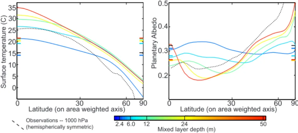
4b. Planetary albedo and the globally and annually averaged temperature 379
The meridional structure of the annual mean planetary albedo is dramatically dif-380
ferent in the shallow and deep ocean mixed layer depth experiments. In the deep 381
ocean runs, there is a well defined contrast between the high albedo tropics and low 382
albedo subtropics. In contrast, the shallow ocean runs feature a meridionally broad 383
high albedo tropical region. The meridional extent of the high planetary albedo trop-384
ical region expands poleward as the depth of the ocean mixed layer decreases (right 385
panel of Figure 6). The extratropical planetary albedo is highest for the deeper mixed 386
layer depth runs and is a consequence of a seasonally persistent mid-latitude baro-387
clinic zone and storm track in the deep runs. In contrast the mid-latitude baroclinic 388
zone and storm track only exists in the winter in the shallow ocean runs; in the shallow 389
ocean runs, the extratropical storm track vanishes along with the barcolinity during 390
the summer months (the maximum SSTs are found between 40◦and 50◦). As a result,
391
there are fewer clouds and lower extratropical planetary albedo in the annual mean 392
in the shallow runs. The differences in tropical and extratropical planetary albedo 393
across the suite of ocean mixed layer depth simulations partially but far from com-394
pletely compensate for one another in the global average with the tropical response 395
dominating the global mean behavior. The global mean planetary albedo for each 396
simulation is shown by the thick horizontal lines on the right and left axes of the right 397
panel of Figure 6. The global mean planetary albedo increases with decreasing mixed 398
layer depth and varies by 0.05 across the suite of simulations which corresponds to 399
a global mean top of the atmosphere (TOA) shortwave radiation difference of 15 W 400
m−2. We note that, the seasonal covariance of planetary albedo and insolation makes
401
a negligible contribution to the annual and global mean planetary albedo in all runs 402
(i.e. the seasonal insolation weighted annual mean albedo is comparable to the annual 403
mean albedo in all regions). 404
The zonal and annual mean SST differs greatly across the suite of slab ocean 405
aquaplanet simulations (left panel of Figure 6) and are a consequence of the differ-406
ences in global mean planetary albedo. The global average SST is 7C higher in the 407
50m ocean slab depth run than in the 2.4m slab depth run which is significantly colder 408
than the other runs. Overall, the differences in global mean surface temperature across 409
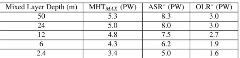
the suite of simulations follow the global mean absorbed shortwave radiation (ASR 410
= S[1 − αP]) with a 2 W m−2increase in ASR corresponding to an approximately 1
411
degree C increase in global mean temperature. The low-latitude SSTs (equatorward 412
of 30◦) increase monotonically with increasing mixed layer depth concurrent with the
413
decrease in local planetary albedo. In contrast, the differences in extratropical SST 414
across the suite of experiments do not follow the differences in local ASR. For ex-415
ample, the extratropics of the 2.4m run are the coldest of the entire ensemble despite 416
the fact that the local planetary is the lowest amongst all the ensemble members. This 417
result suggests that the global mean energy balance is communicated to all regions 418
of the globe by way of the (atmospheric) meridional energy transport, regardless of 419
the local radiative differences. We further pursue the changes in meridional energy 420
transport in the next section. 421
5. Meridional energy transport and jet location 422
In the previous section, we demonstrated that the meridional structure of planetary 423
albedo differs drastically across the suite of slab ocean aquaplanet simulations. The 424
equator-to-pole gradient of planetary albedo plays a fundamental role in determin-425
ing the meridional heat transport in the climate system (Stone 1978; Enderton and 426
Marshall 2009). The mid-latitude heat transport is primarily accomplished by eddies 427
in the atmosphere (Czaja and Marshall 2006) and the eddies affect the jet location 428
and the surface winds (Edmon et al. 1980). Therefore, any change in the magnitude 429
and/or spatial structure of meridional heat transport is expected to be accompanied 430
by a shift in the jet. In this section, we demonstrate that there are first order changes 431
in the annual mean meridional heat transport and zonal winds across the suite of slab 432
ocean aquaplanet simulations. 433
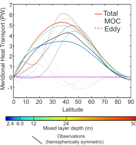
5a. Meridional energy transport 434
The annually averaged meridional energy transport in the slab ocean aquaplanet sim-435
ulations is shown in Figure 7. We note that, there is no ocean energy transport in 436
these simulations which allows the atmospheric energy transport to be calculated 437
from spatially integrating the net radiative imbalance at the TOA from pole to pole. 438
The contribution of the mean overturning circulation (MOC – i.e. the Hadley and 439
Ferrel cells) to the energy transport is calculated from the monthly mean meridional 440
velocity, temperature, specific humidity and geopotential field using the advective 441
form of the energy flux equation as in Donohoe and Battisti (2013). The eddy contri-442
bution is calculated as the total energy transport minus the MOC energy transport3.
443
3 The stationary eddies make a negligible contribution to the total energy transport. The stationary eddy
The peak in energy transport is almost 2 PW higher in the deep ocean runs (5.4 PW in 444
the 50m simulation) as compared to the shallow ocean runs. The meridional structure 445
of the energy transport is more meridionally peaked for the deep runs as compared to 446
the flatter structure seen for the shallow runs. 447
The partitioning of the energy transport into MOC and eddy components shows 448
several anticipated features (Figure 7). In the low latitudes, the energy transport is 449
dominated by a poleward energy transport in the thermally direct Hadley cell4 and
450
the eddies make a negligible contribution (with the exception of the deep tropics 451
of the 50m run). The Hadley cell energy transport extends farther poleward in the 452
shallow runs due to the expansion of the tropics that was previously noted. In the 453
mid-latitudes, the eddies dominate the total energy transport and the MOC energy 454
transport is equatorward in the thermally indirect Ferrel cell. The peak equatorward 455
energy transport in the Ferrel cell is co-located with the eddy energy transport maxi-456
mum in all runs which is consistent with the Ferrel cell being driven by the eddies. 457
The reduced meridional energy transport in the shallow mixed layer depth runs 458
(relative to deep runs) is accompanied by weaker eddy energy transport in the mid-459
latitudes (c.f. the blue and red dashed lines in Figure 7). From the perspective of the 460
TOA radiation budget, the increased subtropical planetary albedo in the shallow run 461
results in a smaller magnitude net radiative surplus and demands weaker eddy energy 462
flux divergence and therefore weaker mid-latitude eddies; the weaker eddies result 463
from a reduced meridional gradient in shortwave heating between the subtropics and 464
the extratropics. From the perspective of the local dynamics, the mid-latitude baro-465
clinity in the shallow runs is severely reduced during the summer as the maximum 466
SSTs are found around 40◦. As a result, the mid-latitude storm track essentially
dis-467
appears (along with the baroclinity) during the summer in the shallow runs whereas 468
the storm track is nearly seasonally invariant in the deep runs. The seasonal variations 469
in storm track intensity and location results in weaker eddies in the annual mean in 470
the shallow runs as compared to the deep runs. We note that, the eddy energy flux 471
maximum is shifted 10◦poleward in the 2.4m run as compared to the 50m run
(peak-472
ing at 47◦as compared to 37◦). This shift is a consequence of the differences in the
473
meridional extent of the Hadley cell energy transport and differences in the total heat 474
transport demanded by the TOA radiation budget as a consequence of the changes 475
in subtropical planetary albedo associated with the seasonal migration of the Hadley 476
cell (see Figure 6). The ramifications of the reduced and poleward shifted eddies in 477
the shallow run will be further discussed in Section 55b. 478
The maximum meridional energy transport between the tropics and the extratrop-479
ics (MHTMAX) is equal to the net radiative deficit at the TOA spatially integrated over
480
the extratropics (Trenberth and Caron 2001). As such, it can be thought of as the ASR 481
anomaly relative to the global mean integrated over the extratropics (ASR∗) minus the
482
outgoing longwave radiation anomaly integrated over the same region (OLR∗– see
483
Donohoe and Battisti 2012, for a discussion): 484
4 The equatorward MOC energy transport in the deep tropics of the 50m run is a consequence of the
moist static energy decreasing with height in the boundary layer due to a very moist and warm boundary layer. This results in the Hadley cell transporting energy in the same direction as the meridional flow at the surface.
MHTMAX= ASR∗− OLR∗. (4)
ASR∗is a consequence of the meridional gradient in incident radiation and the
merid-485
ional gradient of planetary albedo. The latter was shown in Section 44b to differ sub-486
stantially with ocean mixed layer depth with a larger meridional gradient in planetary 487
albedo for the deep ocean runs (c.f. the red and blue lines in the right panel of Figure 488
6). One would therefore expect the deep ocean runs, with a stronger meridional gra-489
dient in planetary albedo, to have enhanced meridional energy transport(MHTMAX)
490
provided that the spatial gradients in absorbed radiation (ASR∗) are not completely
491
balanced by local changes in emitted radiation (OLR∗). In physical terms, when the
492
extratropics have a higher planetary albedo than the tropics, the equator-to-pole con-493
trast of energy input into the climate system is enhanced (ASR∗increases) and the
494
system must balance the enhanced gradient in absorbed insolation by fluxing more 495
energy from the tropics to the extratropics (increasing MHTMAX) or by coming to
496
equilibrium with a larger equator to pole temperature gradient resulting in a larger 497
OLR gradient by the Planck feedback (increasing OLR∗). ASR∗increases from 5.0
498
PW in the 2.4m depth run to 8.3 PW in the 50m depth run (Table 1) and the ma-499
jority of the changes in ASR∗ are balanced by enhanced energy transport into the
500
extratropics (MHTMAX) while changes in OLR∗play a secondary role in balancing
501
differences in ASR∗across the suite of simulations. This result suggests that
differ-502
ences in the equator-to-pole gradient in absorbed shortwave radiation are primarily 503
balanced by changes in the dynamic energy transport and secondarily by local ra-504
diative adjustment (by way of the Planck feedback). This result is consistent with 505
the findings of Donohoe and Battisti (2012) and Enderton and Marshall (2009) who 506
found that changes in the meridional structure of planetary albedo are mainly bal-507
anced by changes in the total meridional energy transport in the climate system. 508
5b. Zonal jets and surface winds 509
In the previous section, we found that deepening the ocean mixed layer resulted in 510
an increase and equatorward shift of the annual mean eddy energy flux as a conse-511
quence of the changes in tropical planetary albedo and the associated total energy 512
transport change demanded by the equator-to-pole scale energy budget at the TOA. 513
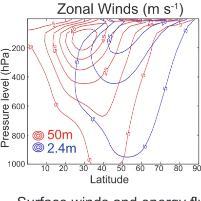
Here, we examine the relationship between the eddy energy flux and the zonal jet and 514
surface winds across the suite of slab ocean aquaplanet simulations. Figure 8 shows 515
the cross sections of the annually and zonally averaged zonal winds for the 50m run 516
(red) and the 2.4m run (blue). The upper tropospheric jet in the 50m run is stronger 517
in magnitude, and shifted equatorward by approximately 15◦latitude relative to its
518
counterpart in the 2.4m run. The jet shift extends all the way to the surface where the 519
winds are more than twice the magnitude and shifted 15◦equatorward in the 50m run
520
as compared to the 2.4m run. 521
The intensity and location of the surface winds across the ensemble of slab ocean 522
aquaplanet simulations are readily understood given the changes in the eddy energy 523
fluxes that were discussed in Section 55a. The acceleration of the zonal winds is 524
equal to the divergence of the Eliassen-Palm flux (F– Eliassen and Palm 1961). At the 525
surface, ∇ · F (and F) is dominated by the vertical component (Andrews and McIntyre 526
1976) which is proportional to the eddy energy flux. Neglecting the horizontal (eddy 527
momentum flux) component of the Eliassen-Palm flux, the acceleration of the zonal 528
wind at the surface is: 529 ∂USU RF ∂ t ≈ f ∂ ∂ p V∗hθ∗+CL Pq ∗i σ0 (5)
(Stone and Salustri 1984) where V is the meridional velocity, θ is the potential tem-530
perature, q is the specific humidity,∗denotes the eddy component and [ ] is the zonal
531
and time average of the eddy covariance. σ0 is the basic state static stability, f is
532
the Coriolis parameter and p is pressure. Conceptually, the meridional eddy energy 533
flux (moist static energy) accelerates the zonal flow by acting as a form drag on isen-534
tropic surfaces (Vallis 2006). We note that, this derivation assumes that the basic state 535
stratification is substantially larger than the spatial variability of the static stability, 536
and thus, the impact of the spatially varying static stability on zonal jet is neglected 537
in this theory and the discussion below. The argument of the pressure derivative is 538
the eddy (moist static) energy flux. Provided that there is no energy flux at the sur-539
face, and the eddy energy fluxes vary smoothly in the vertical, peaking somewhere in 540
the troposphere, the zonal acceleration of the winds in the lower troposphere will be 541
proportional to the vertically integrated meridional energy flux. The dominant mo-542
mentum balance at the surface is between the eddy acceleration of the zonal winds 543
and the frictional damping at the surface. Provided that the frictional damping is pro-544
portional to the surface winds, the surface winds should be proportional to and peak 545
at the same location as the maximum in eddy energy flux. 546
The annual and zonal average eddy energy flux is co-plotted with the the surface 547
winds for the suite of slab ocean aquaplanet simulations in the lower panel of Figure 548
8. We note that the zonal average eddy energy flux that appears in Equation 5 and Fig-549
ure 8 differs from the zonally integrated energy flux that is shown in Figure 7 by the 550
zonal circumference at each latitude. The latter contains a factor of the cosine of lat-551
itude and thus the zonally averaged eddy energy flux peaks poleward of the zonally 552
integrated energy flux which is constrained by the spherical geometry of the Earth 553
(Stone 1978). In all simulations, the maximum surface westerlies are co-located with 554
the peak in the eddy energy flux (c.f. the red and black lines in the lower panel of 555
Figure 8). The maximum eddy energy flux in the 2.4m depth run is located approxi-556
mately 15◦poleward of its counterpart in the 50m run and the jet shifts meridional by
557
approximately the same distance. The meridional structure and relative amplitudes 558
of the surface westerlies across the suite of simulations also mimic the differences 559
in the eddy energy flux. These results collectively suggest that Equation 5 and the 560
approximations discussed in the paragraph above are a reasonable, albeit simplistic 561
representation of the system behavior. The location of the maximum surface winds re-562
spond to the vertically averaged eddy energy fluxes which themselves are constrained 563
by the equator-to-pole scale radiative budget. 564
6. Summary and discussion 565
The amplitude of the seasonal cycle in temperature and energy fluxes increases with 566
decreasing ocean mixed layer depth in suite of slab ocean aquaplanet simulations. 567
This expected behavior is accompanied by several less intuitive results including: 1. 568
the phase of the seasonal cycle in temperature varies non-monotonically with ocean 569
mixed layer depth (bottom left panel of Figure 1), 2. the tropics are more meridionally 570
expansive in the shallow depth runs (lower panel of Figure 5), 3. the annual and global 571
mean surface temperature is of order 5C lower in the shallow runs as compared to the 572
deep runs (left panel of Figure 6), 4. the mid-latitude meridional energy transport is 573
reduced by of order 50% in the shallow runs (Figure 7) and 5. the zonal winds shift 574
poleward by more than 10◦in the shallow mixed layer depth runs (Figure 8). Below,
575
we review the mechanisms responsible for these results and discuss the behaivor of 576
the observed climate system relative to the suite of aquaplanet mixed layer depth 577
simulations. 578
The seasonal heating of the atmosphere can be decomposed into two contribu-579
tions: the sun heating the surface and the surface subsequently fluxing energy to the 580
atmosphere by turbulent and longwave energy fluxes (SHF), and the sun directly 581
heating the atmosphere by shortwave absorption (SWABS) in the atmospheric col-582
umn (Donohoe and Battisti 2013). The surface fluxes dominate the seasonal heating 583
of the atmosphere in the shallow ocean runs while the entirety of the seasonal heating 584
of the atmosphere is due to SWABS in the deeper ocean runs (Figure 3). The surface 585
contribution to the seasonal heating of the atmosphere has a larger phase lag relative 586
to the insolation for the deeper runs, and this explains the initial increase in phase 587
lag of atmospheric temperature as the mixed layer depth increase from 2.4m to 12m. 588
However, as the mixed layer depth increases beyond 12m, the seasonal heating of the 589
atmosphere becomes increasingly dominated by SWABS, which is in phase with the 590
insolation, and the total heating of the atmosphere comes back into phase with the 591
insolation. The phase of seasonal variations in temperature and energy fluxes across 592
the suite of aquaplanet simulations and the observations are readily explained by the 593
phase of atmospheric heating (bottom panel of Figure 4). 594
The net seasonal heating of the observed climate system is dominated by SWABS 595
in both hemispheres (purple lines in Figure 3) with the exception of the mid-latitude 596
continents (Donohoe and Battisti 2013). The observed phase lag of the atmospheric 597
temperature relative to the insolation is smaller than even in the 2.4m slab ocean 598
simulations. We note that, the phase of the total atmospheric heating relative to the 599
insolation in the observations is also smaller than that in the aquaplanet simulations 600
and that the phase of atmospheric temperature is well predicted given the phase of 601
the atmospheric heating (c.f. the red diamonds with the black diamonds in the lower 602
panel of Figure 4). The cause of the smaller phase lag between the insolation and the 603
net atmospheric heating in the observations relative to the aquaplanet simulations is 604
unclear and we speculate on the possible causes below. One possibility is that, the 605
presence of land with a near zero heat capacity over even a small subset of the do-606
main sets the phase of atmospheric heating and temperature over the whole domain. 607
Because the land surface has such a small heat capacity, seasonal variations in down-608
welling shortwave radiation are transferred to the overlying atmosphere with near 609
zero-phase lag. This source of energy input into the atmosphere is communicated 610
hemispherically by way of the atmospheric advection with a time scale of order one 611
week (Donohoe 2011) and a fraction even ends up in the ocean mixed layer (Donohoe 612
and Battisti 2013). Thus, the land surface serves as a large input of energy into the 613
atmosphere with near zero phase lag and could set the phase of temperature over the 614
entire globe. It is possible that even the small amount of land in the Southern Hemi-615
sphere sets the phase of seasonal variations in temperature above the Southern Ocean 616
which also exhibits a pronounced phase lead of temperature relative to the aquaplanet 617
simulations (Figure 2). Other possible explanations for the discrepancy between the 618
model and the observations include, the seasonal cycle of ocean circulation (e.g. the 619
ocean energy flux convergence over this region), the seasonal shoaling of the thermo-620
cline, the role of sea-ice cover (sea-ice is prohibited from forming in the aquaplanet 621
simulations), and an inadequate representation of the turbulent energy fluxes in the 622
model. 623
In simple, linear, energy balance models, the heat capacity of the climate sys-624
tem has no affect on the annual mean climate since there is no energy storage in 625
equilibrium. We have demonstrated that, the ocean mixed layer depth has a profound 626
affect on the annual mean climate in a suite of aquaplanet simulation. The mixed 627
layer depth’s influence on the annual mean climate is a consequence of the seasonal 628
seasonal migration of the ITCZ and it’s impact on planetary albedo and can be ex-629
plained as follows. The enhanced seasonal cycle of SSTs and atmospheric energy 630
fluxes in the shallow mixed layer experiments results in the ITCZ migrating farther 631
off the equator seasonally (top panel Figure 5). As the ITCZ moves off the equator, 632
an asymmetry between the winter and summer Hadley cells develops resulting in a 633
broad region of ascent and convective precipitation in the summer hemisphere and 634
extensive stratus in the winter hemisphere. The time average of the seasonally mi-635
grating ITCZ in the shallow ocean runs is a very weak annual mean Hadley cell with 636
precipitation and high planetary albedo broadly spread over the low-latitudes. This 637
is a stark contrast to the deeper ocean runs where ascending branch of the Hadley 638
cell is confined to within 10◦of the equator (during all seasons) resulting in a small
639
region of convective precipitation and high planetary albedo and a well defined dry 640
and cloud free subtropical region. The Tropics expand and broaden in the shallow 641
mixed layer depth runs resulting in a high global mean planetary albedo. As a result, 642
the annual mean temperature decreases in the shallow runs (Figure 6). The enhanced 643
planetary albedo in the shallow runs is confined to the tropics which results in a de-644
creased equator-to-pole gradient of absorbed shortwave radiation and reduced merid-645
ional energy transport (Figure 7). The peak in eddy energy transport is both reduced 646
and shifted poleward in the shallow ocean runs which results in a poleward shift and 647
weakening of the eddy-driven jet (Figure 8). This sequence of causality emphasizes 648
that clouds play a central role in determining both the global mean and spatial pattern 649
of ASR and, therefore, the large scale atmospheric circulation. 650
These results suggest that an adequate representation of the seasonal cycle is im-651
portant for modeling the extent of the tropics, the global mean energy budget and 652
the magnitude of the mid-latitude atmospheric energy transport and its effect on the 653
jets. The observed seasonal migration of the ITCZ is comparable to that of the 12m 654
or 24m mixed layer depth simulation (see Donohoe et al. 2013, Figure 8). Similarly, 655
the strength of the annual mean Hadley cell and meridional structure of the plane-656
tary albedo and precipitation in the observed climate system is comparable to that of 657
the 12m slab ocean aquaplanet simulation. In comparison, the strength of the annual 658
mean Hadley in the 50m simulation is a factor of four larger than the observations 659
(bottom panel of Figure 5) and the annual mean precipitation and planetary albedo 660
barely peaks in the tropics in the 2.4m run. Clearly, the seasonal migration of the 661
ITCZ makes an impact on mean climate in the observations and, if the magnitude of 662
the seasonal cycle is unreasonable, the basic state climate, including the extratropical 663
atmospheric circulation, will not be adequately represented. Thus, one should be cau-664
tious when interpreting results from climate simulations forced by annual mean (or 665
equinoctial insolation) or seasonal slab ocean simulations with extreme mixed layer 666
depths. 667
Acknowledgements AD was funded by the NOAA Global Change Postdoctoral Fellowship.
668
References 669
Andrews, D. and M. McIntyre, 1976: Planetary waves in horizontal and vertical shear: 670
The generalized eliassen-palm relation and the zonal mean acceleration. J. Atmos. 671
Sci., 33, 2031–2048. 672
Chiang, J. and A. Friedman, 2012: Extratropical cooling, interhemispheric thermal 673
gradients, and tropical climate change. Annu. Rev. Earth Planet. Sci., 40, 383–412. 674
Chou, M. and K. Lee, 1996: Parameterizations for the absorption of solar radiation 675
by water vapor and ozone. J. Atmos. Sci., 53, 1203–1208. 676
Czaja, A. and J. Marshall, 2006: The partitioning of poleward heat transport between 677
the atmosphere and the ocean. J. Atmos. Sci., 63, 1498–1511. 678
Danabasoglu, G. and P. Gent, 2009: Equilibrium climate sensitivity: is it accurate to 679
use a slab ocean model? J. Climate, 22, 2494–2499. 680
Delworth, T. L., A. J. Broccoli, A. Rosati, R. J. Stouffer, V. Balaji, J. A. Beesley, and 681
W. F. Cooke, 2006: Gfdl’s cm2 global coupled climate models. part i: Formulation 682
and simulation characteristics. J. Climate, 19, 643–674. 683
Donohoe, A., 2011: Radiative and dynamic controls of global scale energy fluxes. 684
Ph.D. thesis, University of Washington, 137 pp. 685
Donohoe, A. and D. Battisti, 2012: What determines meridional heat transport in 686
climate models? J. Climate, 25, 3832–3850. 687
— 2013: The seasonal cycle of atmospheric heating and temperature. 688
Donohoe, A., J. Marshall, D. Ferreira, and D. McGee, 2013: The relationship between 689
itcz location and atmospheric heat transport across the equator: from the seasonal 690
cycle to the last glacial maximum. J. Climate, in press. 691
Edmon, J., H. J., B. Hoskins, and M. McIntyre, 1980: Eliassen-palm cross sections 692
for the troposphere. J. Atmos. Sci., 37, 2600–2616. 693
Eliassen, A. and E. Palm, 1961: On the transfer of energy in staionary mountain 694
waves. 695
Enderton, D. and J. Marshall, 2009: Controls on the total dynamical heat transport of 696
the atmosphere and oceans. J. Atmos. Sci., 66, 1593–1611. 697
Table 1 The peak poleward energy transport (MHTMAX) and its partitioning into the extratropical deficit
in absorbed shortwave (ASR∗) and emitted longwave radiation (OLR∗) in the slab ocean aquaplanet
sim-ulations.
Mixed Layer Depth (m) MHTMAX(PW) ASR∗(PW) OLR∗(PW)
50 5.3 8.3 3.0
24 5.0 8.0 3.0
12 4.8 7.5 2.7
6 4.3 6.2 1.9
2.4 3.4 5.0 1.6
Fasullo, J. T. and K. E. Trenberth, 2008a: The annual cycle of the energy budget: Part 698
1. global mean and land-ocean exchanges. J. Climate, 21, 2297–2312. 699
— 2008b: The annual cycle of the energy budget: Part 2. meridional structures and 700
poleward transports. J. Climate, 21, 2313–2325. 701
Frierson, D., Y. Hwang, N. Fuckar, R. Seager, S. Kang, A. Donohoe, E. Maroon, 702
X. Liu, and D. Battisti, 2013: Why does tropical rainfall peak in the northern hemi-703
sphere? the role of the oceans meridional overturning circulation. Nature, submit-704
ted. 705
Johanson, C. and Q. Fu, 2009: Hadley cell widening: model simulations versus ob-706
servations. J. Climate, 22, 2713–2725. 707
Kang, S., I. Held, D. Frierson, and M. Zhao, 2008: The response of the itcz to extra-708
tropical thermal forcing: idealized slab-ocean experiments with a gcm. J. Climate, 709
21, 3521–3532. 710
Lin, S. J., 2004: A ”vertically lagrangian” finite-volume dynamical core for global 711
models. Mon. Weath. Rev., 132, 2293–2307. 712
Lindzen, R. and A. Hou, 1988: Hadley circulations of zonally averaged heating cen-713
tered off the equator. J. Atmos. Sci., 45, 2416–2427. 714
North, G. R., 1975: Theory of energy-balance climate models. J. Atmos. Sci., 32, 715
2033–2043. 716
Rose, B. and D. Ferreira, 2013: Ocean heat transport and water vapor greenhouse in a 717
warm equable climate: a new look at the low gradient paradox. J. Climate, in press. 718
Schneider, E. K., 1996: A note on the annual cycle of sea surface temperature at the 719
equator. Technical Report. Center for Ocean-Land-Atmosphere Studies, 18 pages. 720
Stone, P., 1978: Constraints on dynamical transports of energy on a spherical planet. 721
Dyn. Atmos. Oceans, 2, 123–139. 722
Stone, P. and G. Salustri, 1984: Generalization of the quasi-geostrophic eliassen-palm 723
flux to include eddy forcing of condensational heating. J. Atmos. Sci., 41, 3527– 724
3535. 725
Trenberth, K. E. and J. M. Caron, 2001: Estimates of meridional atmosphere and 726
ocean heat transports. J. Climate, 14, 3433–3443. 727
Vallis, G. K., 2006: Atmospheric and Oceanic Fluid Dynamics.. Cambridge Univer-728
sity Press. 729
Wielicki, B., B. Barkstrom, E. Harrison, R. Lee, G. Smith, and J. Cooper, 1996: 730
Clouds and the earth’s radiant energy system (CERES): An earth observing system 731
experiment. Bull. Amer. Meteor. Soc., 77, 853–868. 732
30 40 50 60 70 80 90 0 5 10 15 20 25 30 35 40 45 Latitude
Seasonal Amplitude of temperature
2.4 6 12 24 50
Mixed layer depth (m)
30 40 50 60 70 80 90 50 55 60 65 70 75 80 85 90 95 100 Latitude
Seasonal phase lag of temperature (days relative t
2.4 6 12 24 50 80 90 70 60 50 40 Latitude 2.4 6.0 12 24 50
Seasonal amplitude of temperature (K) 0
5 10 15 20 25 30 35 40 45 30 40 50 60 70 80 90 20 30 40 50 60 70 80 90 Latitude
Seasonal phase lag of temperature (days r
e 2.4 6 12 24 50 80 90 70 60 50 40 Latitude
Phase of tropospheric average temperature (phase lag relative to solsticew in days)
50 60 70 90 Amplitude Phase Surface 600 hPa 80 40 30 20 30 40 50 60 70 80 90 0 5 10 15 20 25 30 35 40 45 Latitude
Seasonal Amplitude of temperature
2.4 6 12 24 50 80 90 70 60 50 40 Latitude
Seasonal amplitude of temperature (K) 0
5 10 15 20 25 30 35 40 45 30 40 50 60 70 80 90 20 30 40 50 60 70 80 90 Latitude
Seasonal phase lag of temperature (days r
e 2.4 6 12 24 50 80 90 70 60 50 40 Latitude
Phase of tropospheric average temperature (phase lag relative to solstice in days)
50 60 70 90 Amplitude Phase 80 40 30 20
Aquaplanet Models Observations
NH Surface NH 600 hPa SH Surface SH 600 hPa NH SH
Fig. 1 (Top) The seasonal amplitude of atmospheric temperature at the surface (solid lines) and at 600 hPa (dashed lines) in the slab-ocean aquaplanet simulations (Left Panel) and observations (Right Panel). The different ocean mixed layer depths are indicated by the colorbar below the plot. (Bottom) Phase lag of seasonal cycle of tropospheric averaged(below 250 hPa) temperature with respect to insolation in the slab-ocean aquaplanet simulations (Left) and observations (Right). The phase lag is expressed in days past the summer solstice.
Latitude 40 50 60 70 80 900 700 500 300
Pressure Level (hPa)
2.4 Meters 6 Meters
24 Meters 12 Meters
50 Meters
Seasonal Phase of Temperature
Seasonal phase lag of temperature (days after solstice)
70 50 30 Latitude 40 50 60 70 80 900 700 500 300
Pressure Level (hPa)
Latitude 40 50 60 70 80 900 700 500 300
Pressure Level (hPa)
Latitude 40 50 60 70 80 900 700 500 300
Pressure Level (hPa)
Latitude 40 50 60 70 80 900 700 500 300
Pressure Level (hPa)
Observations SH Latitude 80S 900 700 500 300
Pressure Level (hPa)
70S 60S 50S 40S Observations NH Latitude 80N 900 700 500 300
Pressure Level (hPa)
70N 60N 50N 40N
90 110
Fig. 2 Meridional-height cross sections of the phase of the seasonal cycle of atmospheric temperature in each of the slab-ocean aquaplanet simulations (upper panels) and the observations (lower panels). Values are expressed as the phase lag relative to the insolation in days.
JAN FEB MAR APR MAY JUN JUL AUG SEP OCT NOV DEC
Seasonal anomaly of extraropical energy fl
ux (W m -2) -50 0 50 100
JAN FEB MAR APR MAY JUN JUL AUG SEP OCT NOV DEC
JAN FEB MAR APR MAY JUN JUL AUG SEP OCT NOV DEC -50 0 50 100 100 200 -100 0 Atmospheric Absorption Surface Heating Total Heating
Mixed layer depth (m) Latitude
2.4 6.0 12 24 50
NH Observations SH Observations (+1/2 year)
Fig. 3 Time series of atmospheric heating averaged over the Northern Extratropics defined as poleward of
40◦N. The total atmospheric heating (bottom panel) is decomposed into contributions from solar
absorp-tion in the atmospheric column (SWABS–top) and surface energy fluxes (SHF–middle panel). The annual mean value of each contribution has been subtracted from the time series. The different ocean mixed layer depths are indicated in the colorbar at the bottom and the observations in the Northern and Southern hemi-sphere are shown by the solid and dashed purple lines respectively. The SH curve has been shifted by half a year. The vertical dashed lines represent the phase of the seasonal cycle and the vertical dashed black line is the summer solstice.
SWABS Surface Heating Column Tendency OLR
Heat Transport div.
Seasonal amplitude of extratropical energy fl uxes
Normalized amplitude of annual harmonic of extratropical
energy fl ux in phase with total heating
-1.0 -0.5 0 0.5 1.0 1.5
Slab ocean depth (m)
2.46 12 24 50 NH Obs. SH Obs. SWABS SHF Storage OLR ∆∙ Heat Trans.
Phase of extratropical energy fl uxes and temperature
Seasonal phase of energy fl ux/temperature
(days of lag past summer solstice)
0 20
Slab ocean depth (m)
2.46 12 24 50 NH Obs. SH Obs. 40 60 80 100 -20 -40 -60 Atmos. Heating Storage ∆∙ Heat Trans. OLR Temperature
Fig. 4 (Top Panel) The normalized seasonal amplitude of energy fluxes to the extratropics, defined as the amplitude of the annual harmonic in phase with the total atmospheric heating (SWABS + SHF). The amplitude is normalized by the amplitude of the total heating to demonstrate the relative amplitude of the terms in the different mixed layer depth experiments. (Bottom Panel) The phase of the various energy flux terms in the extratropics. The temperature is the atmospheric column integrated temperature. The red and black dashed vertical lines represent the solstice and equinox respectively.

![[PDF] Cours Microsoft Word 2007 comment ça marche | Cours informatique](data:image/gif;base64,R0lGODlhAQABAIAAAP///wAAACH5BAEAAAAALAAAAAABAAEAAAICRAEAOw==)