Effect of gas path heat transfer on turbine loss

Effect of Gas Path Heat Transfer on Turbine Loss

by

Thomas J. Kleiven

Submitted to the Department of Aeronautics and Astronautics

in partial fulfillment of the requirements for the degree of

Master of Science in Aeronautics and Astronautics

at the

MASSACHUSETTS INSTITUTE OF TECHNOLOGY

June 2017

Massachusetts Institute of Technology 2017. All rights reserved.

Author

....

Signature redacted

Department of Aeronautics and Astronautics

May 25, 2017

Certified

by.

Signature redacted...

Edward M. Greitzer

H.N. Slater Professor of Aeronautics and Astronautics

Certified by.

Accepted by ....

MASSACHUSETTS INSTITUTE OF TECHNOLOGYL.

JUL 11

2017

Signature redacted

Thesis Supervisor

Choon S. Tan

Senior Research Engineer

Thesis Supervisor

Signature redacted

I/"

Youssef M. Marzouk

Associate Professor of Aeronautics and Astronautics

Chair, Graduate Program Committee

w

Effect of Gas Path Heat Transfer on Turbine Loss

by

Thomas J. Kleiven

Submitted to the Department of Aeronautics and Astronautics on May 25, 2017, in partial fulfillment of the

requirements for the degree of

Master of Science in Aeronautics and Astronautics

Abstract

This thesis presents an assessment of the impact of gas path, i.e., streamtube-to-streamtube, heat transfer on aero engine turbine loss and efficiency. The assessment, based on the concept of mechanical work potential

[19],

was carried out for two model problems to introduce the ideas. Three-dimensional RANS calculations were also conducted to show the application to realistic configurations. The first model prob-lem, a constant area mixing duct, demonstrates the importance of selecting a fluid component loss metric appropriate to the purpose of the overall system in which the component resides. The phenomenon of thrust increase due to mixing is analyzed to show that system performance can increase even though there is a loss of ther-modynamic availability. Gas path heat transfer affects mechanical work potential, and thus turbine loss, through a mechanism called thermal creation

[19].

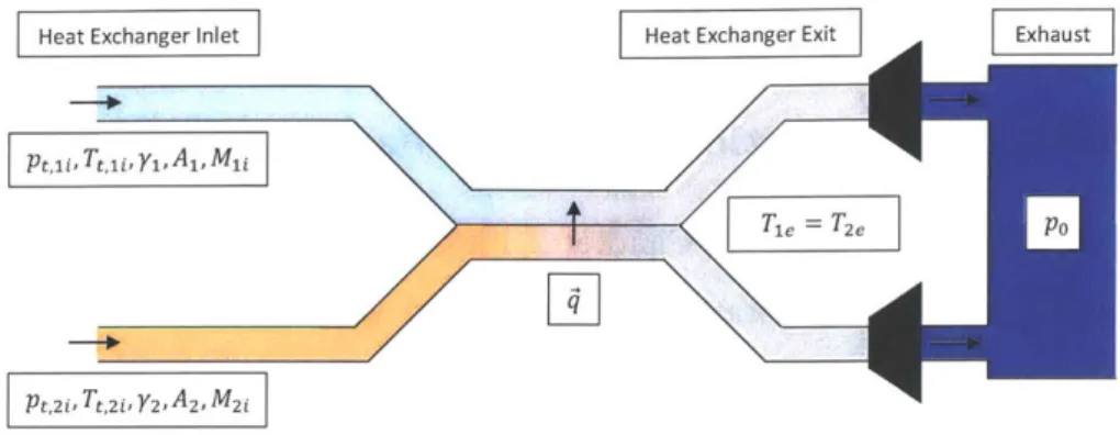
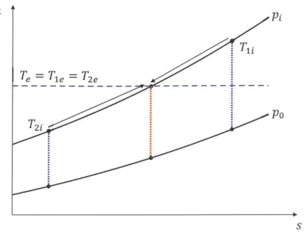
The second model problem, an inviscid heat exchanger, illustrates how thermal creation is due to enthalpy redistribution between flow regions with different local Brayton efficiency. Heat transfer across a static pressure difference, or between gases with different spe-cific heat ratios, can cause turbine efficiency to increase or decrease depending on the direction of the heat flow. Three-dimensional RANS calculations have also been interrogated to define and determine the thermal creation, and thus the losses, in a modern two-stage cooled high pressure turbine. At representative engine operating conditions the effect of thermal creation was a 0.1% decrease in efficiency, with the thermal creation accounting for 1% of the overall lost work. Introducing coolant flow into the main gas path increased the loss from thermal creation in the first stage by 84% and decreased the loss from thermal creation in the second stage by 8%.

Thesis Supervisor: Edward M. Greitzer

Title: H.N. Slater Professor of Aeronautics and Astronautics Thesis Supervisor: Choon S. Tan

Acknowledgments

This research was carried out with the generous support of the Rolls-Royce Whittle Fellowship. The research is the result of a close collaboration between the MIT Gas Turbine Lab and the Turbine Aerodynamics group at Rolls-Royce North America.

I would like to thank my advisors, Professor Ed Greitzer and Dr. Choon Tan, for their guidance and encouragement throughout my time at MIT; this work would not have been possible without their insightful questions and constructive feedback.

I am also indebted to Professor Rob Miller from the Whittle Lab, University of Cambridge, who was always willing to discuss my research and served as an invaluable resource for all things mechanical work potential. I would also like to thank Professor Nick Cumpsty and Dr. Graham Pullan, whose helpful comments were particularly valuable in the early stages of the research.

I am grateful for the support of the engineers at Rolls-Royce North America, who were generous with their time and were always willing to assist me. In particular, I would like to acknowledge Jon Ebacher and Bill Cummings, who provided guidance and industry perspective throughout the project, and Tyler Gillen, who taught me the dark arts needed to use HYDRA.

My GTL experience would not have been the same without the friendship and support of my lab mates. Thanks for two years of great food and semi-delirious late night conversations.

I am very grateful for my family. To my parents, thank you for encouraging me to pursue my dreams and for giving me the freedom to do so. To my ridiculously smart and competitive sister, Kimberly, thank you for driving me to always be better.

Last but not least I want to thank Whitney; I would not be where I am today without you. Even with 1,000 miles between us you were able to understand me and encourage me like no one else could. In the most difficult moments I could always look forward to the next time we would be together, and the thought never failed to put a smile on my face. I cannot wait to discover what adventures our future has in store.

Contents

1 Introduction and Background

1.1 Research Questions . . . . 1.2 Methodology . . . . 1.3 Contributions . . . . 1.4 Organization of Thesis...

2 Loss Assessment Methodologies

2.1 Introduction . . . .

2.2 Mixing Duct Model . . . . 2.2.1 The Mixed-Out State . . . .

2.2.2 Boundary Conditions . . . . 2.3 Mixing Loss Metrics . . . . 2.3.1 Availability . . . . 2.3.2 Mechanical Work Potential . . . . 2.3.3 Ideal Specific Gross Thrust . . . . 2.4 Relation of Loss Metrics to Averaged Stagnation 2.5 Gross Thrust Changes from Mixing . . . .

2.5.1 Thrust Balance for Constant Area Nozzles . . . 2.5.2 Thrust Increase for Constant Mass Flow Nozzles

2.6 Summary and Conclusions . . . .

3 Inviscid Model for Turbine Work Changes from Heat Transfer

3.1

Introduction . . . .

23 26 26 27 28 29 29 29 30 30 32 33 36 41 43 45 48 50 52 53 53 Pressures

. .

. .

3.2 Low Mach Number Heat Transfer . . . . 54

3.2.1 Entropy Generation with No Change in Turbine Work . . . . 56

3.2.2 Heat Transfer with Static Pressure Difference . . . . 56

3.2.3 Heat Transfer with Specific Heat Ratio Difference . . . . 59

3.3 Constant Pressure Heat Exchanger . . . . 61

3.4 Constant Area Heat Exchanger . . . . 63

3.5 Thermal Creation with Uniform Inlet Flow . . . . 67

3.6 Summary and Conclusions . . . . 69

4 Quantifying Thermal Creation in an Uncooled Turbine

71

4.1 Introduction . . . .

71

4.2 Computational Approach . . . . 72

4.2.1

Geometry and Mesh . . . .

72

4.2.2 Boundary Conditions . . . . 72

4.3 Methods to Compute Mechanical Work Potential Efficiency . . . . 74

4.3.1 Integrating Fluxes . . . . 74

4.3.2 Evaluation of Volumetric Source Terms . . . . 75

4.3.3 Comparison to Work-Averaged Stagnation Pressure Efficiency 76 4.4 Changes in Turbine Efficiency due to Thermal Creation . . . . 79

4.5 Identifying Thermal Creation Mechanisms . . . . 79

4.6 Summary and Conclusions . . . . 84

5 Quantifying Thermal Creation in a Cooled Turbine

85

5.1 Introduction . . . . 85

5.2 Computational Approach . . . . 86

5.2.1 Geometry and Mesh . . . . 86

5.2.2 Boundary Conditions . . . . 87

5.3 Efficiency Changes from Thermal Creation . . . . 90

5.4 Sources of Highest Thermal Creation . . . . 91

5.4.1 Impact of Cooling Flows on Thermal Creation . . . . 95

5.4.2 Impact of Inlet Turbulence on Thermal Creation . . . . 99

5.5 Summary and Conclusions . . . .1

6 Summary, Conclusions, and Recommendations for Future Work

103

6.1 Summary and Conclusions ... 103

6.2 Recommendations for Future Work ... ... 104

A Thrust Increase from Mixing

107

A .1 Introduction . . . . 107

A.2 Incremental Thrust Changes Due to Mixing . . . . 109

A.3 Thrust Benefit for Complete Mixing . . . . 112

A.4 Effect of Mixing on Efficiency . . . . 113

A.4.1 Overall Efficiency . . . . 113

A.4.2 Thermal Efficiency . . . . 114

A.4.3 Propulsive Efficiency . . . . 115 100

List of Figures

2-1 Constant area mixing of two streams to a uniform exit state [5]. . . 30

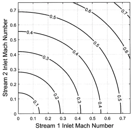
2-2 The representative inlet Mach number, Mi, as a function of stream 1 and stream 2 inlet Mach numbers, M, and M2, for -y = 1.4. . . . . 32

2-3 An ideal process to obtain the maximum work (equal to the change in availability from state i to e) on an h-s diagram. . . . . 35 2-4 Entropy rise coefficient A9 = Tt(se - s)/T 2 for two stream constant

area mixing, with JV = 0.5 and -y = 1.4, as a function of stream inlet stagnation pressure and temperature differences. . . . . 36 2-5 The ideal process when using mechanical work potential analysis shown

on an h-s diagram . . . . . 37 2-6 The ideal process used to define availability [12], modified to show the

mechanical work potential ideal process. . . . . 38 2-7 Loss of mechanical work potential

[%]

due to mixing for M = 0.5,

y = 1.4, and po = i as a function of inlet stagnation temperature difference and inlet stagnation pressure difference. . . . . 39 2-8 Normalized inlet velocity difference (ui - u2)/1(ui + u2) as a function

of stagnation temperature and pressure difference for Mi = 0.5 and

y = 1.4 . . . . . 40

2-9 Loss of ideal specific gross thrust

[%]

due to mixing for Mi = 0.5,

= 1.4, and po = pi. Negative loss indicates an increase in ideal

specific gross thrust due to mixing. . . . . 42 2-10 Availability-averaged stagnation pressure loss [%] due to mixing for

2-11 Work-averaged stagnation pressure loss [%] due to mixing for Mi = 0.5, and y = 1.4. . . . . 46

2-12 Thrust-averaged stagnation pressure loss

[%]

due to mixing for Mi = 0.5, y = 1.4, and po = Pi... . . . .. 47 2-13 Mass-averaged stagnation pressure loss

[%]

due to mixing for Mi = 0.5,

and y = 1.4. . . . . 47

2-14 Gross thrust with mixing, normalized by unmixed gross thrust, for a fixed area subsonic nozzle with uniform inlet stagnation pressure,

Po = 2pt,, and y = 1.4. . . . . 50 2-15 Gross thrust with mixing, normalized by unmixed gross thrust, for

a fixed mass flow, variable area subsonic nozzle with uniform inlet

stagnation pressure, po = iPt,, and y = 1.4. Comparison of low Mach number analysis and numerical evaluation for inlet Mach numbers up to 0 .5 . . . . . 5 1

3-1 Inviscid heat exchanger upstream of isentropic turbines exhausting to the same static pressure, po. . . . . 55 3-2 h-s diagram for heat transfer between streams of equal pressure and

specific heat ratio. . . . . 57 3-3 _{Change in work due to heat transfer with pressure difference. EL" = 4,}

PO

71 = 72 = 1.3, Mi = M2 << 1 n1 = n2. . . . . 58

3-4 h-s diagram for heat transfer at constant static pressure between streams with equal specific heat ratio and a difference in static pressure. . . . 59

3-5 Change in work due to heat transfer with specific heat ratio difference.

P= 4,pi p₂ , =7 1.3, Mi = M2 << 1,i = h2. . . . . . . . 60

3-6 h-s diagram for heat transfer at constant static pressure between streams with a difference in specific heat ratio and equal static pressure. . . . 61 3-7 Change in turbine work normalized by heat transferred for a constant

pressure heat exchanger with inlet pressure difference, E _P2 = 4, 7 =

3-8 Change in turbine work normalized by heat transferred for a constant pressure heat exchanger with specific heat ratio difference, ? _PO = 4,

P1

=

P2,=

1.

3_{, Mli = M}

2 , ri = T2.

. . . .

63 3-9 Change in work from heat transfer with pressure difference, inlet Mach

number = 0.3 in constant area heat exchanger. ELL = 4, 7y1 = -72= 1.3, M ij = M 2j = 0.3, rhi = 42 . . . . . 64 3-10 Change in work from heat transfer with specific heat ratio difference,

inlet Mach number = 0.3 in constant area heat exchanger. E PO = 4,

Pi = Pt,2i, i= 1.3, Mi = M2j = 0.3, rni =r42. . . . . 65

3-11 Contours of Brayton efficiency as a function of pressure ratio and 7.

Changes in Brayton efficiency of streams 1 and 2 due to heat transfer from low efficiency to high efficiency in a constant area heat exchanger with non-negligible inlet Mach number are tracked. . . . . 66 3-12 Contours of Brayton efficiency as a function of pressure ratio and '7.

Changes in Brayton efficiency of streams 1 and 2 due to heat transfer from high efficiency to low efficiency in a constant area heat exchanger

are tracked. ... ... 67 3-13 Schematic of heat transfer in an inviscid flow with uniform upstream

flow. ... ... 68

4-1 View of the structured rotor passage mesh and tip mesh. . . . . 73 4-2 Inlet profile of stagnation temperature normalized by mass-averaged

inlet stagnation temperature, T/Tm, for OTDF = 0.6. [13] . . . . 74 4-3 Difference in turbine efficiency

[%]

between mechanical work potential

efficiency and work-averaged stagnation pressure efficiency as a func-tion of dead state pressure chosen to define mechanical work potential normalized by work-averaged exit stagnation pressure . . . . 78 4-4 Computed changes in turbine efficiency

[%]

as a function of inlet

stag-nation temperature non-uniformity (OTDF) for four efficiency defini-tion s. . . . . 78

4-5 Change in turbine efficiency

[%]

due to thermal creation in the vane and rotor as a function of inlet hot streak OTDF. . . . . 80 4-6 Isosurfaces of thermal creation normalized by volumetric average

vis-cous dissipation, Atherm/4visc, showing regions of largest positive and negative thermal creation for (i) OTDF = 0 and (ii) OTDF = 0.6. . . 81

4-7 Contours on mid-span radial slice with OTDF = 0: (i) thermal creation normalized by volumetric average viscous dissipation (Atherm/ 4visc),

(ii) static pressure term

(

IPc,), (iii) heat flux term

(

7

11

).

. . . 83

P

W/(nrc.,b)

4-8 Contours of the projection of pressure gradient on heat flux vector on a mid-span radial slice for OTDF = 0 (left) and OTDF = 0.6 (right). 84

5-1 Meridional view of the two-stage high pressure turbine with cavities and slot cooling. . . . . 87 5-2 Inlet stagnation temperature normalized by mass-average inlet

stagna-tion temperature, T/T

m

. . . .

88

5-3 Inlet turbulent to laminar viscosity ratio, t/vl. . . . .. . . . 89

5-4 Contributions to lost work in the mixing plane calculation of the cooled turbine first stage. . . . . 92

5-5 Contours of thermal creation normalized by volumetric average viscous

dissipation, Atherm/oDisc, on four r - 0 planes in the cooled first stage

vane. The axial locations are: (i) one axial chord upstream of vane leading edge, (ii) 1% axial chord upstream of vane leading edge, (iii) half axial chord, and (iv) 1% axial chord downstream of vane trail-ing edge. Leadtrail-ing edge and trailtrail-ing edge positions are indicated with dashed lines, and the pressure side (PS) and suction side (SS) are iden-tified . . . . 92

5-6 Contours of thermal creation normalized by volumetric average viscous dissipation, Atherm/visc, on three r - 0 planes in the cooled first stage rotor. The axial locations are: (i) 1% axial chord upstream of rotor

leading edge, (ii) half axial chord, and (iii) 1% axial chord downstream

of rotor trailing edge. Leading edge and trailing edge positions are indicated with dashed lines, and the pressure side (PS) and suction

side (SS) are identified. . . . . 94

5-7 Contours of thermal creation normalized by volumetric average viscous dissipation, Atherm/4Dvisc, on three r - 0 planes in the cooled second stage vane. The axial locations are: (i) 1% axial chord upstream of vane

leading edge, (ii) half axial chord, and (iii) 1% axial chord downstream

of vane trailing edge. Leading edge and trailing edge positions are indicated with dashed lines, and pressure side (PS) and suction side

(SS) are identified. . . . . 94

5-8 Contours of thermal creation normalized by volumetric average viscous dissipation, Atherm/visc, on four r-- planes in the cooled second stage rotor. The axial locations are: (i) 1% axial chord upstream of rotor

leading edge, (ii) half axial chord, (iii) 1% downstream of rotor

trail-ing edge, and (iv) one axial chord downstream of rotor trailtrail-ing edge. Leading edge and trailing edge positions are indicated with dashed lines, and pressure side (PS) and suction side (SS) are identified. . . . 95

5-9 Contours of thermal creation normalized by volumetric average vis-cous dissipation, Atherm/Ivisc, on a mid-span radial slice through the uncooled two-stage turbine. . . . . 96

5-10 Contours of thermal creation normalized by volumetric average viscous dissipation, Atherm /Jvisc, on a mid-span radial slice through the cooled turbine. . . . . 96

5-11 Isosurfaces of

0.1 thermal creation normalized by volumetric average

viscous dissipation,

/4therm/Tvisc, showing regions of highest positive

and negative thermal creation around the first stage rotor suction side

(i) without and (ii) with cooling flow. . . . .

97

5-12 Isosurfaces of

0.1 thermal creation normalized by volumetric average

viscous dissipation, Atherm/Ivisc, showing regions of highest positive

and negative thermal creation around the first stage rotor pressure

side (i) without and (ii) with cooling flow. . . . .

98

A-1 Mixing of fan and core streams in an aero engine propulsion system.

.

108

A-2 Sketch of the mixing duct and nozzle, with nomenclature. . . . .

108

List of Tables

3.1 Streamtube area, Mach number, and mass average mechanical work potential at each station for -y = 1.3, Mi = 0.3, Po = !Pt,i. . . . . 69

5.1 Nodes in the two-stage turbine mesh. . . . . 88 5.2 Sources of coolant flow, as a percentage of combustor exit mass flow rh4. 90

5.3 Change in efficiency from thermal creation, Artc, in the two-stage tur-bine with and without cooling flows. . . . . 90

Nomenclature

Acronyms

CFD computational fluid dynamics

OTDF overall temperature distribution function PS pressure side

RANS Reynolds-Averaged Navier-Stokes

RTDF radial temperature distribution function SA Spalart-Allmaras

SS suction side

SST shear stress transport

TSFC thrust specific fuel consumption ID one-dimensional

Roman Symbols

A area

b availability

b span

cP specific heat at constant pressure

cX axial chord

D corrected flow function

DP non-dimensionalized stagnation pressure difference DT non-dimensionalized stagnation temperature difference F gross thrust

Fnet net thrust

h enthalpy

k turbulent kinetic energy

M Mach number

rh mass flow rate

mf mechanical work potential

(mf)oss mechanical work potential loss metric

Mi representative inlet Mach number

nr number of rotor passages

p pressure

PR stagnation-to-static pressure ratio

T-- arithmetic average stagnation pressure (Pt)loss stagnation pressure loss metric

q[ heat flux vector

R specific gas constant

r radial coordinate

s entropy

T temperature

TR stagnation temperature ratio

Tt arithmetic average stagnation temperature

u velocity magnitude

U* ideal specific gross thrust

(u*1)i10 , ideal specific gross thrust loss metric

Ui representative inlet velocity a, v, w x,y,z components of velocity

V volume

w work

W turbine power

W10 ts lost work

maximum shaft work cartesian coordinates

non-dimensional wall cell distance

a

'7 Atherm

Ah

fuel As Asirreversible 70 rip 77source 2th 'T7wa 7o

0

vi p projection angle proportionality constant specific heat ratio

arithmetic average specific heat ratio change in a quantity

thermal creation

heat of combustion of fuel non-dimensional entropy rise irreversible entropy change

change in turbine efficiency from thermal creation turbulent dissipation

efficiency

turbine efficiency based on mechanical work potential fluxes overall efficiency

propulsive efficiency

turbine efficiency based on mechanical work potential sources thermal efficiency

turbine efficiency based on work-averaged stagnation pressure turbine efficiency with OTDF = 0

circumferential coordinate dynamic viscosity laminar viscosity turbulent viscosity density [Wshaft]max x, y, z

Greek Symbols

- bypass ratio jic viscous dissipation

vDjc volumetric average viscous dissipation

w turbulence dissipation rate

Subscripts

c core

e exit station

f

fan

i inlet station

ref reference state

se isentropic turbine exit state

t stagnation quantity

0 surrounding state

1,2,ect. stream number 1,2,ect. station number

Superscripts

a averaged quantity ba availability-averaged m mass-averaged ta thrust-averaged wa work-averaged

Chapter 1

Introduction and Background

Large thermal gradients exist within the gas path of an aero engine high pressure turbine, due to hot streaks and coolant flows. These temperature non-uniformities create the potential for substantial heat transfer in the gas path'. At the turbine inlet, hot streaks from the combustor result variations of stagnation temperature by 20% of the mass-averaged value [15]. The coolant flows, which are used to keep the vane and rotor metal temperatures enough below melting so the material properties have acceptable values, are injected into the main gas path and exchange heat with the hot flow exiting the combustor. In this thesis we examine the turbine efficiency changes associated with gas path heat transfer and address the connection between entropy generation and turbine efficiency.

In Denton's classic paper on loss mechanisms [5], he makes the connection between losses in turbomachinery and increases in entropy; an increase in entropy from heat transfer between fluid streams with a finite temperature difference results in lost work and an efficiency decrease. In the same paper, however, Denton includes an model of a cooled turbine where the entropy generated from heat transfer between coolant streams and the main gas path flow has no impact on turbine efficiency. It is this issue on which we focus.

In a high pressure turbine, the entropy generated from gas path heat transfer

'In this thesis, gas path heat transfer refers to the heat transferred streamtube-to-streamtube in the main gas path of a turbomachine.

can be of the same order as that generated from viscous dissipation. Jedamski [13] assessed the change in efficiency of a single stage turbine with increasing hot streak strength. He found that the efficiency change between a turbine with uniform inlet stagnation temperature and a turbine with a non-uniform inlet stagnation tempera-ture was sensitive to the choice of efficiency definition. If a definition based on the availability averaged stagnation pressure was used, in which all increases in entropy contribute to loss, a turbine with an OTDF2 _{= 0.6 hot streak has 6% lower efficiency} than one with uniform inlet. Jedamski argues that efficiency should instead be based on a mixed-work definition, using a work-averaged inlet stagnation pressure and a mixed-out average exit stagnation pressure for which the efficiency decrease due to the hot streak is less than 1%.

Lim et al. [17j assessed turbine loss associated with injecting film cooling air into the main gas path and found that turbine efficiency decreases by 8.0% if all entropy generation is considered a loss. They advocate adopting a "pragmatic approach" where irreversibility associated with heat transfer is neglected, however, and the decrease in turbine efficiency is 0.7%.

Young and Horlock

[23]

described several definitions for cooled turbine efficiency. They argue that the fully reversible mixed efficiency should be used, in which the actual turbine power is compared to the maximum power that could possibly be ex-tracted from the flow. In such an ideal process, Carnot cycles are used to reversibly bring all inlet streams to a common stagnation pressure and stagnation tempera-ture, after which the streams are mixed and expanded through an isentropic turbine. This definition is similar to the "rational efficiency" based on availability, and it also accounts for the increase in work possible when gases with different specific heat ra-tio are mixed. From this perspective, all irreversibility results in a loss of turbine

efficiency [23].

Another ideal process was also proposed by Young and Horlock [23] to determine a weighted-pressure mixed efficiency. That efficiency considers thermal mixing of inlet streams to be inevitable, and recognizes that in aero engine turbines work cannot be

2OTDF is a measure of temperature distortion and is defined as max(Tt 4(r )-Tt. Tt,4 - t,3

extracted from the temperature difference between streams. The ideal process used is thus irreversible and includes the "minimum practical thermal entropy production." Only if the change in entropy is greater than the minimum practical thermal entropy production does lost work result.

To analyze cooled turbines, Hartsel [101 used an efficiency where the actual turbine work is compared to an ideal process where each inlet stream undergoes separate isentropic expansion to the exhaust static pressure. The ideal turbine work is given by the sum of the kinetic energies of each stream following expansion to the exhaust pressure. No explicit link between gas path heat transfer and changes in turbine efficiency was given.

Miller

[19]

has provided a rigorous definition for turbine efficiency based on the concept of mechanical work potential, defined as the turbine work possible when ex-panding a fluid isentropically to a dead state pressure with zero velocity. In this framework the actual turbine work is compared to the sum of the changes in mechan-ical work potential of each stream, which is equivalent to the turbine work obtained by expanding isentropically from the inlet state to the exit state. This efficiency def-inition is equal to the one proposed by Hartsel [10], and if the dead state pressure is taken equal to the turbine exit static pressure, the inlet mechanical work potential is equal to Hartsel's ideal work.

Miller [19] also showed that changes in mechanical work potential are possible by exchanging heat or work with the surroundings, and by two internal mechanisms: viscous dissipation and thermal creation. Only entropy generated from viscous dissi-pation contributes to lost turbine work. The effect of streamtube-to-streamtube heat transfer on turbine efficiency is captured by thermal creation (investigated in detail in Chapter 3), which can be positive or negative depending on the angle between the local static pressure gradient and the heat flux vector. Thermal creation can result in a mechanical work potential efficiency, or equivalently, Hartsel efficiency, that exceeds unity.

1.1

Research Questions

The goal of this work is to quantify the changes in turbine efficiency from gas path heat transfer. The selection of an appropriate metric to characterize turbine loss and the application of mechanical work potential to adiabatic high pressure turbine flows are addressed. The specific research questions are:

" What is the correct loss metric for aero engine high pressure turbines and what are the implications of the choice?

" Under what conditions is thermal creation significant compared to turbine work? " How large is thermal creation in the main gas path of a high pressure turbine? " What is the effect of inlet hot streaks and coolant flows on thermal creation in

a high pressure turbine?

1.2

Methodology

To address the research questions, a combination of model problems and three-dimensional RANS CFD has been carried out. Analysis of a constant area mixing duct with three different downstream processes is used to highlight the importance of selecting the appropriate loss metric. Discussion of ideal processes relevant for aero engine turbines aids in this selection. Analysis of the inviscid heat exchanger proposed by Miller [19] isolates the effect of heat transfer on turbine work, and serves to help explain the thermal creation mechanism.

Thermal creation is evaluated in a high pressure turbine stage and compared to viscous dissipation and turbine work. The effect of inlet hot streaks on thermal creation is defined for an idealized hot streak with OTDF up to 0.6. The effect of a more representative turbine inlet profile, obtained from combustor CFD, on thermal creation is then examined for a two-stage high pressure turbine. The thermal creation due to the addition of cooling flows to the main gas path is also evaluated and compared with the other mechanisms for turbine loss.

1.3

Contributions

The main contributions of this work are:

" Miller's argument [19] that mechanical work potential should be used when an-alyzing aero engine turbines instead of approaches based on entropy, i.e. avail-ability, is supported by several different model problems including gas path heat transfer. An example of thrust increase from mixing upstream of a nozzle is used to demonstrate the importance of using different loss metrics for fluid components depending on the purpose of the overall system.

" Changes in turbine efficiency due to thermal creation of 10% are found for an inviscid heat exchanger with static pressure differences or specific heat ratio differences. The efficiency change is caused by a redistribution of the enthalpy of the flow between regions of differing Brayton efficiency [20] based on static pressure.

" The impact of thermal creation on turbine efficiency for a representative un-cooled high pressure turbine stage is determined to be less than 0.01%, re-gardless of inlet stagnation temperature non-uniformity. With or without hot streaks, the highest local thermal creation is due to the rotor tip leakage flow. * The impact of thermal creation on efficiency for a representative two-stage,

cooled high pressure turbine is determined to be -0.1%. Adding coolant flow to the main gas path approximately doubles the change in efficiency from thermal creation in the first stage. Even with coolant flow, thermal creation comprises only 1% of the overall lost work in the high pressure turbine.

" The sensitivity of thermal creation to inlet turbulence has been shown. Using a turbine inlet profile taken from combustor CFD at engine operating conditions, with inlet turbulent to laminar viscosity ratio of 1,000, the thermal creation is approximately 10 times higher than when an inlet boundary condition with turbulent viscosity ratio of 100 is used.

1.4

Organization of Thesis

The first part of this thesis supports the use of mechanical work potential and thermal creation [191 to quantify the effect of gas path heat transfer on turbine loss. In Chapter 2, an analysis of mixing with three different processes occurring downstream is used to demonstrate the importance of selecting the correct loss metric. One process, thrust augmentation from mixing, shows a situation in which, even though there can be an entropy increase, the mixing can lead to enhanced performance (thrust). In Chapter 3, the mechanism of thermal creation, is investigated for an inviscid heat exchanger to show how heat transfer between streams with differing static pressure or specific heat ratio leads to changes in turbine work.

The second part of the thesis quantifies changes in turbine efficiency due to gas path heat transfer. In Chapters 4 and 5, mechanical work potential analysis is applied to three-dimensional turbine flows. The impact of thermal creation on efficiency is found for an uncooled high pressure turbine stage and for a cooled two-stage high pressure turbine. The impact of inlet turbulence and of coolant flows on thermal creation is assessed. Mechanisms for thermal creation in three-dimensional flows are discussed, and regions of the flows with highest thermal creation are identified.

Chapter 6 provides a summary of the key results from Chapters 2-5 and provides recommendations for future work on turbine efficiency changes due to heat transfer.

Chapter 2

Loss Assessment Methodologies

2.1

Introduction

A rigorous loss quantification is necessary to analyze and mitigate mechanisms that reduce system performance. As described by Cumpsty and Horlock, there are a number of choices for loss metrics in internal flow [4] that arise from comparing the real process to one that is idealized in some way. One choice is to consider a reversible process as the ideal, but other choices can be made in which irreversibility is included

[23]. It is well known that an upper bound on loss exists, given by availability in the sense of the maximum amount of lost work for a given passage from one state to another [12] [14]. However, such a metric is not useful in many situations, including aero engine high pressure turbine flows [191, in which there is no opportunity for reversible heat exchange downstream of the process of interest. In what follows we demonstrate this by evaluating the mixing loss for two streams in a constant area duct with different downstream processes.

2.2

Mixing Duct Model

The model problem to be described is constant area mixing of two co-flowing streams as in Figure 2-1. This allows us to show how the interpretation of loss for the same physical process depends on the overall purpose of the system. The flow has two

streams of an ideal gas with stagnation pressures pt,i and

Pt,2,

stagnation temperatures

T,

1

and

T,2,

and areas A

1

and A

2

that enter an adiabatic, constant area duct. To focus

on the mixing process we neglect wall shear and assume that streamline curvature

induced by mixing is negligible so the pressure across the mixing duct is uniform.

The flow mixes between station i (inlet) and station

e

(exit) with a uniform state at

e

that has stagnation pressure pt,e, stagnation temperature Tte, and Mach number Me.

m'pa

Uniform

mixing

flow

p.L _{A pi, Tte}

P121 Tt2 o

Figure 2-1: Constant area mixing of two streams to a uniform exit state 151.

2.2.1

The Mixed-Out State

Conditions at the mixed-out state can be found using a control volume from mixing

duct inlet to mixing duct exit and applying the one-dimensional (1D) conservation

equations of mass, momentum, and energy for a steady flow in an adiabatic constant

area duct with wall shear neglected

151.

The mixed-out mass flow is the sum of inlet

mass flows. Conservation of energy means that the mass flux of stagnation enthalpy

at the inlet and exit are the same, so, the mixed out stagnation temperature is

determined. The mixed-out Mach number is found from the 1D momentum equation.

The mixed-out stagnation pressure and entropy are then given from the mass flow

rate, stagnation temperature, area, and Mach number.

2.2.2

Boundary Conditions

We follow the procedure of Denton

151

to set the non-dimensional boundary conditions.

In the examples to be worked out, we take the areas of the two streams to be equal.

The inlet stagnation temperature boundary condition is set by choosing DT, the

stagnation temperature difference between the two inlet streams non-dimensionalized by

t,

the arithmetic average of the stagnation temperatures (Equations 2.1 and 2.2),

DT=

T,

T,2 (2.1)

T

T=

(T,

+

T,2). (2.2)

The inlet stagnation pressure boundary condition is given by DP, the inlet stagnation pressure difference normalized by the difference between the arithmetic average inlet stagnation pressure - and the mixing duct inlet static pressure (Equations 2.3 and 2.4),

DP

= Pt,i -Pt,2 (2.3)

Pt

-

A

PTi

(Pt,1

+ Pt,2).- (2.4)

The duct inlet static pressure and hence the Mach number of each stream is set by specifying a representative inlet Mach number,

Mi,

based on the average stagnation pressure as in Equation 2.5,

F- = Pi)(1 + 2 Mi (2.5)

Using Equations 2.3, 2.4, 2.5, and the total to static pressure ratio of each stream, the representative inlet Mach number is given as a function of the stream 1 and stream 2 Mach numbers in Equation 2.6,

(1 + Y M22

_(2.6)

Given

Mi,

stream inlet Mach numbers M1 and M2 can be found as a function of

DP. With uniform duct inlet stagnation pressure (DP = 0) the Mach number in both streams is Mi. Contours of Mi are provided in Figure 2-2 using -y = 1.4 and varying the individual stream Mach numbers from 0 to 0.75. The mixed-out state is

determined by specifying DT, DP, MN, and -y.

E

Z Ca CN

E

z

0 0.7 0.6 0.5 0.4 0.3 0.2 0.1 0

NK

0.4 -04

9->

0

N

o

C C

1.

0 0.1 0.2 0.3 0.4 0.5 0.6 0.7

Stream

1

Inlet Mach Number

Figure 2-2: The representative inlet Mach number, Mi, as a function of stream 1 and stream 2 inlet Mach numbers, M1 and M2, for y 1.4.

2.3

Mixing Loss Metrics

The mixing process can have different impacts on the overall system performance depending on the use of the flow downstream of the mixing region. The mixing duct will be considered here as a part of three different systems, and an appropriate loss metric will be defined for each system. The first class of problems considered is work extraction where both pressure and temperature differences between the fluid and the surroundings can be used to obtain work. An example is a co-generation power plant [121, where work is obtained from (i) a turbine expanding flow to the surrounding pressure, and (ii) downstream heat engines in which the flow can exchange heat with the surroundings. The second situation is one in which work can be obtained only

through a pressure difference between the fluid and surroundings. An example is an aircraft engine turbine, which generates work by expanding the flow to a lower pressure, but which does not provide an opportunity for generation of additional work through heat exchange with the surroundings. The third example is one in which the flow is used to produce thrust as in the flows immediately upstream of and internal to a propelling nozzle.

2.3.1

Availability

When the maximum work that is possible to extract from a flow for a given state change (or the minimum amount of work required) is of interest, the change in avail-ability is the appropriate loss indicator [12]. Availavail-ability measures the maximum use-ful work that can be extracted from a flow undergoing a state change in a reversible process in which there is heat exchange with one or more heat reservoirs.

The availability for a steady flow can be defined from application of the first and second laws of thermodynamics to a control volume with heat addition and shaft work. Equation 2.7 states the first law for a control volume, where the shaft work output is equal to the heat input plus the decrease in stagnation enthalpy from state

1 to state 2,

Wshaft= q + (ht1 - ht2). (2.7)

For a fluid stream exchanging heat only with an environment at temperature, To, the change in entropy from state 1 to state 2 is given by the difference between (i) irre-versible entropy generated inside the volume and (ii) heat rejected to the surroundings divided by the temperature of the surroundings1_,

(s₂ - Si) - A = Asirreversible > 0. (2.8)

TO

Combining Equations 2.7 and 2.8 yields an expression for shaft work as a function of the change in the quantity ht - Tos, from state 1 to state 2, and the irreversible

entropy generated inside of the control volume multiplied by the temperature of the surroundings (Equation 2.9),

Wshaft (ht - Tos)1 - (ht - Tos)2 - TOASirreversible. (2.9)

The quantity ht - Tos, denoted by the symbol b, is defined as the flow availability

[12],

b = ht - Tos.

(2.10)

The irreversible entropy generation must be greater than or equal to zero, and Equation 2.9 thus means that maximum shaft work occurs when ASirreversible = 0, corresponding to a reversible process from states 1 to 2 and reversible heat transfer. The decrease in availability is equal to the shaft work extracted in this ideal process. The difference between the shaft work extracted in the ideal process and the actual shaft work extracted for the change between state 1 and state 2 is the work lost due to irreversibility. Equation 2.11 expresses the actual shaft work in terms of the change

in availability and the lost work, TOASirreversible,

Ws9haft = A - TOASirreversible = [Wshaft~max - Wl₀st- (2.11)

To extract work reversibly between two states we can expand the flow from the initial pressure to the final pressure using an isentropic turbine, and then bring the flow to the final temperature using a Carnot cycle. For flow with uniform stagnation pressure and temperature this process is shown in an h-s diagram in Figure 2-3. The flow is first expanded from the inlet state, i, to the isentropic turbine exit state, se. It is then brought to the exit state, 0, using a series of Carnot cycles to exchange heat with the surroundings.

In the mixing duct there is no shaft work so, from Equation 2.11, the lost work is equal to the change in availability from inlet to exit. Further, because the mixing duct is adiabatic, entropy changes from inlet to exit must be due to irreversible entropy generation, and the entropy rise is proportional to the lost work. The entropy rise

Ptji

PO

---- --- -...-- ...--- s -- Tt,se

~--

_{-- ~---~~~---~~~~---~~~----}

TO

0

S

Figure 2-3: An ideal process to obtain the maximum work (equal to the change in availability from state i to e) on an h-s diagram.

coefficient in Equation 2.12 is a non-dimensional metric for entropy generation in the adiabatic mixing duct. It is defined by multiplying the change in entropy by the arithmetic average stagnation temperature Tt and dividing by a representative inlet specific kinetic energy 7j-2 (Equation 2.13) based on a flow velocity defined by the arithmetic average stagnation temperature Tt and the reference inlet Mach number

A = Tt(e (2.12)

-T -= . (2.13)

1+ 12 Y-1-22i

Figure 2-4 shows the entropy rise coefficient for M= 0.5 and y = 1.4 as a function of inlet stagnation temperature difference and inlet stagnation pressure difference. Note that DT = 1 is equivalent to a stagnation temperature ratio T,1/T, 2 = 3.

For uniform inflow, there is no entropy change. As the stagnation pressure and stagnation temperature non-uniformities increase, the entropy generated in mixing tends to increase. With inlet stagnation temperature difference |DTI > 0.5,

increas-ing the inlet stagnation pressure difference can lead to lower entropy generation. This is due to the competition of the two processes for entropy generation: viscous dissipa-tion, driven by differences in velocity, and internal heat transfer, driven by differences in static temperature. Increasing the stagnation pressure difference for positive DT decreases the static temperature difference and increases the velocity difference. For the higher values of DT shown, this trade-off leads to a decrease in mixed-out entropy.

1 0.8 0.6 0.4 0.2 T1 -Tt2 _

~(Ttl

Tt,2) 0 -0.2 -0.4 -0.6 -0.8 -1.5 -1 -0.5 0 0.5 1 1.5 Pti -Pt2

Figure 2-4: Entropy rise coefficient A9 = Tt(se - si)/ i- for two stream constant area2 mixing, with Mi = 0.5 and -y = 1.4, as a function of stream inlet stagnation pressure and temperature differences.

When there is a possibility for the system to take advantage of heat transfer with the surroundings to generate work, the change in availability is an appropriate loss benchmark and the lost work, proportional to irreversible entropy generation, is the appropriate loss metric.

2.3.2

Mechanical Work Potential

For situations in which no heat can be exchanged with the surroundings, it is not ap-propriate to use an ideal process which includes extracting work from the temperature

-0-0.2

--

0--0 0.5

difference between system and surroundings for analysis of the maximum work that

can be obtained. Put another way, the reversible processes used to define

availabil-ity are not a useful benchmark for these situations. Following Miller

1191,

the ideal

process for such adiabatic systems is taken to be work extraction through isentropic

expansion to the pressure of the surroundings and zero velocity. The flow mechanical

work potential per unit mass, mf 1191, is defined in Equation 2.14. The mechanical

work potential is a function of enthalpy h, pressure p, velocity u, and a chosen dead

state pressure po, equal to the pressure of the surroundings which the fluid reaches at

the end of the isentropic expansion,

U i2 mf =

h 1 -(P)

+

-.

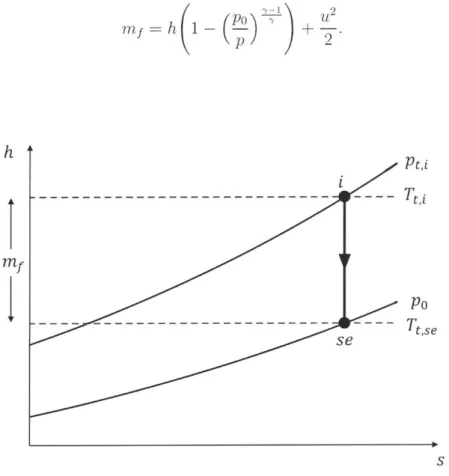
(2.14)

h

Pt

tt

--- ----

Tt' i

mf

Po

.. _ _ _ -------

Tt~se

se S

Figure 2-5: The ideal process when using mechanical work potential analysis shown

on an h-s diagram.

We can write Equation 2.14 for a perfect gas with constant specific heats in terms

of stagnation quantities to give the flow mechanical work potential as the change in

stagnation enthalpy from expansion to the isentropic exhaust state,

mf

= cPTt 1 -

(O

)

'

ht

-

hse.

(2.15)

This state change is indicated in an h-s diagram in Figure 2-5 by considering a fluid

with initial state i. A decrease in flow mechanical work potential represents a decrease

in the isentropic work that can be obtained.

Figure 2-6 presents a second representation of the reversible ideal processes used to

define mechanical work potential by modifying a commonly used representation of the

availability ideal process. The work obtainable using a reversible Carnot cycle is not

relevant to mechanical work potential; the ideal work only consists of work obtained

by reversible processes in the control volume (i.e., with an isentropic turbine).

Extended control volume C+ = control volume C + auxiliary cyclic devices

Specified Specified

inlet state Rigid control volume exit state

C

- ' Internally reversible process

pl, T, H1, S, P2, T2, H21 S2 (WR)REV I(Q[)W 12 (X )REV I ' (QO)REV)' Conceptual environment To, PO

Figure 2-6: The ideal process used to define availability [12], modified to show the

mechanical work potential ideal process.

We can analyze the mixing duct problem using the decrease in mechanical work

potential as the metric. A work potential loss metric, (mf),,,,, is defined in Equation

2.16 as the change in mechanical work potential flux from mixing duct inlet to mixing duct exit normalized by the inlet mechanical work potential flux,

(mf)IosS

-J'(mf)edrh

-

Jf(mf) drh

f(mf)idrh

(2.16)

If we specify an ambient pressure po, and ratio of specific heats 'y, we can find the change in mechanical work potential for a control volume. For specified Mi, y, and

po, the loss in mechanical work potential is a function of the inlet stagnation

temper-ature and stagnation pressure non-uniformities. The mechanical work potential loss, expressed as a percentage, is given in Figure 2-7 for Mi = 0.5, -y = 1.4, and po = Pi.

-1.5 -1 -0. 5 0 0 Pti -Pt2

Pt1+Pt2)-Pi

.5 1 1.5

Figure 2-7: Loss of mechanical work potential

[%]

due to mixing for Mi = 0.5, y = 1.4, and po = p as a function of inlet stagnation temperature difference and inlet stagnation pressure difference.

Unlike loss based on availability, mechanical work potential loss does not always increase with increasing inlet stagnation temperature non-uniformity. Combinations of non-uniform stagnation temperatures and pressures (for example, points A and B in Figure 2-7) exist such that there is no mixing loss from the mechanical work potential metric, even though entropy is generated. For these conditions, the amount

0.8 0.6 0.4 0.2 Ttl1-Tt2 ' (Tt1+Tt2 ) -0.2 -0.4 -0.6 -0.8 -1 - -P 0\ 0

-B\

of work that can be extracted from the flow is unchanged by the mixing process. Miller [19] details the physical mechanisms that change the mechanical work po-tential. One mechanism is entropy generation from viscous dissipation, i.e., conver-sion of mechanical energy to internal energy. A second mechanism, termed thermal

creation, arises when the heat flux vector and the static pressure gradient are

non-orthogonal. For the mixing duct problem, the static pressure at the inlet face is assumed uniform and the static pressure gradient along the duct is not taken into ac-count, so the change in mechanical work potential is due to viscous entropy generation only.

To estimate the viscous mixing losses, we examine the velocity difference between the streams at the inlet to the mixing duct. Figure 2-8 shows the velocity difference between the two streams at mixing duct inlet, normalized by the arithmetic average inlet velocity, as a function of inlet stagnation pressure non-uniformity and inlet stagnation temperature non-uniformity. As previously, Mi = 0.5 and -y = 1.4. Points A and B are marked in the same locations as in Figure 2-7, and correspond to zero inlet velocity difference.

0.8 0.6 0.4 0.2 Tt1--Tt2-S(Tt1+Tt2 ) 0 -0.2 -0.4 -0.6 -0.8 1 -1.5 -1 -0.5 0 0.5 1 1.5 Pt -Pt2

Figure 2-8: Normalized inlet velocity difference (u1 - U2)/!(Ui + U2) as a function of

stagnation temperature and pressure difference for Mi = 0.5 and y = 1.4. A0

10-- V

-. .. .

-The mechanical work potential loss observed in Figure 2-7 increases as the mag-nitude of the inlet velocity difference increases, suggesting that mechanical work po-tential losses are driven by inlet velocity differences. For matched inlet velocities

(Ua = u2), the mechanical work potential loss is exactly zero, even though the inlet

stagnation pressure and stagnation temperature are non-uniform. In these cases, en-tropy is generated from streamtube-to-streamtube heat transfer between streams of differing static temperature, but there is no entropy generatiofn from velocity mixing. There would be a loss calculated using an availability analysis, but there is no loss in terms of mechanical work potential.

2.3.3

Ideal Specific Gross Thrust

The third process is related to thrust generation in propulsion systems. For a flow that generates thrust by expanding through a propelling nozzle, the ideal specific

gross thrust furnishes a useful loss metric. As in mechanical work potential analysis,

the ideal process is isentropic, but no shaft work is extracted by the nozzle. The ideal gross thrust per unit mass flow, u*, is equal to the exit velocity attained from isentropic nozzle expansion to ambient pressure, po, as in Equation 2.17,

Pt*

2cpT 1 - - - . (2.17) A loss metric can be defined as in Equation 2.18 as the change in the flux of ideal specific gross thrust from mixing duct inlet to mixing duct exit normalized by the flux of inlet ideal specific gross thrust,

f (U*)jdi - f(u*)edrhi

(u*)1os8 -. . (2.18)

f ( *)idmh

For the same conditions used previously (Mi = 0.5, -y = 1.4, and po = ) the ideal specific gross thrust change, expressed as a percentage, is given for a range of inlet stagnation temperature and stagnation pressure non-uniformities in Figure 2-9.

-2 0 1 0.8 0.6 0.4 0.2 T1 --Tt2 S(Tt1+Tt2 ) 0 -0.2 -0.4 -0.6 -0.8 -1 -1.5 -1 -0.5 0 Pti -Pt2 -V --0 -2 'X 1N 0.5 1 1.5

Figure 2-9: Loss of ideal specific gross thrust

[%]

due to mixing for Mi = 0.5, -y = 1.4, and Po = p . Negative loss indicates an increase in ideal specific gross thrust due to mixing.

gross thrust in terms of the mechanical work potential. This is done in Equation 2.19, which states that the exit kinetic energy per unit mass flow at the nozzle exit following isentropic expansion is equal to the work that can be extracted with an isentropic turbine,

U =

V

2

mf. (2.19)

The ideal specific gross thrust is proportional to the square root of the mechanical work potential, but processes that lead to changes in ideal specific gross thrust do not necessarily have the same effect on changes in mechanical work potential. To maximize thrust, the exit momentum flux should be maximized, not the exit kinetic energy flux. In the mixing duct, work and heat exchange between two streams with different inlet mechanical work potential increases the mechanical work potential of one stream at the expense of the other. From Figure 2-7, this results in either no change or a net decrease in mechanical work potential. Work and heat exchange be-tween two streams with different ideal specific gross thrust increases the ideal specific

Q

--gross thrust of one stream at the expense of the other, but the net effect can be to

increase or to decrease the specific gross thrust.

An important result is that the contours of ideal specific gross thrust loss are qualitatively different from the contours of mechanical work potential loss. Most notably, the ideal specific gross thrust is increased due to mixing with large normalized stagnation temperature non-uniformity and small stagnation pressure non-uniformity. The thrust increases because, for given heat exchange, the exit velocity of the cold stream (receiving heat) increases more than the exit velocity of the hot stream (losing heat) decreases. This mechanism is responsible for the thrust increase provided by gas turbine engine mixer nozzles that mix cold fan flow and hot core flow [7] [15] [3].

Changes in ideal specific gross thrust are also caused by stagnation pressure losses, from both viscous dissipation and heat transfer. The contours of zero ideal specific gross thrust loss represent the loci of conditions at which the stagnation pressure losses balance the thrust increase from heat transfer.

2.4

Relation of Loss Metrics to Averaged Stagnation

Pressures

To describe the loss for the three types of downstream processes, three different metrics were required. We can also illustrate the loss in terms of stagnation pressure loss due to mixing in the different situations. Cumpsty and Horlock [4] describe the selection of appropriate stagnation pressure averaging schemes and suggest scenarios in which each scheme is useful. They define four averaging methods which we use to compute stagnation pressure loss from mixing duct inlet to mixing duct exit. When the amount of work extracted with a non-adiabatic flow is of interest, they state that the availability-averaged stagnation pressure, defined in Equation 2.20, is the most appropriate choice,

In(p

a ) ln(pt)drh

-

1 )

(T/Tt"'drh.

(2.20)