Disentangling
Time Constant and Time Dependent
Hidden
State in Time Series with Variational
Bayesian
Inference
by
Dylan
Emanuel Centeno Grullon
Submitted
to the Department of Electrical Engineering
and
Computer Science
in
partial fulfillment of the requirements for the degree of
Master of Engineering in Computer Science and Engineering
at
the
MASSACHUSETTS
INSTITUTE OF TECHNOLOGY
September
2019
○
c
Dylan Emanuel Centeno Grullon, MMXIX. All rights reserved.
The
author hereby grants to MIT permission to reproduce and to
distribute
publicly paper and electronic copies of this thesis document
in
whole or in part in any medium now known or hereafter created.
Author . . . .
Department of Electrical Engineering
and Computer Science
September 3rd, 2019
Certified by . . . .
Duane S. Boning
Clarence J. LeBel Professor
Electrical Engineering and Computer Science
Thesis Supervisor
Accepted by . . . .
Katrina LaCurts
Chair, Master of Engineering Thesis Committee
Disentangling
Time Constant and Time Dependent Hidden
State
in Time Series with Variational Bayesian Inference
by
Dylan
Emanuel Centeno Grullon
Submitted to the Department of Electrical Engineering and Computer Science
on September 3rd, 2019, in partial fulfillment of the requirements for the degree of
Master of Engineering in Computer Science and Engineering
Abstract
In this thesis, we design and explore a new model architecture called a Variational Bayes Recurrent Neural Network (VBRNN) for modelling time series. The VBRNN contains explicit structure to disentangle time constant and time dependent dynamics for use with compatible time series, such as those that can be modelled by differen-tial equations with time constant parameters and time dependent state. The model consists of a Variational Bayes (VB) layer to infer time constant state, as well as a conditioned-RNN to model time dependent dynamics. The VBRNN is explored through various synthetic datasets and problems, and compared to conventional meth-ods on these datasets. This approach demonstrates effective disentanglement, moti-vating future work to explore the efficacy of this model in real word datasets.
Thesis Supervisor: Duane S. Boning
Acknowledgments
Through my time at MIT I have received a large amount of support and assistance. Here I would like to acknowledge all those who contributed to my progress both dur-ing work on this thesis and through my time as an undergraduate.
This research was supported under the MIT-IBM Watson AI Lab, as part of the Quest for Intelligence. I am very grateful as none of this work would have been pos-sible without their backing.
I would like to thank Professor Duane Boning, who invited me into his group, guided me through my masters program, and advised me through my entire time at MIT. His direction kept me on track, and his valuable feedback always pushed me forward.
I would like to acknowledge Kyongmin Yeo, my collaborator at IBM Research who helped tremendously in formalizing the problem underlying this thesis as well as providing valuable insight into the direction of the project.
In addition, I would like to thank my parents, who have always been there for me, supporting me emotionally and financially, and to whom I can attribute all my success in life.
To my friends, I am glad I met each and every one of you and am happy you were there as valuable collaborators and fun distractions when the work got to be too much.
Finally, to my dog Sky who tirelessly comforted me through my final and toughest year at MIT.
Contents
1 Introduction 13
1.1 Motivations for Disentanglement in Time Series Analysis . . . 14
1.2 Related Works . . . 16
1.3 General Model Overview . . . 18
2 Theory 21 2.1 Prior Related Theory . . . 21
2.2 Problem Description . . . 24
2.2.1 Generation of 𝑌 . . . 24
2.2.2 Inference of 𝜋 . . . 25
2.2.3 Modelling 𝑌 . . . 26
2.3 Training of the VBRNN . . . 27
2.3.1 Unsupervised Feature Extraction . . . 27
2.3.2 Training Variational Bayes and RNN . . . 28
3 Experimental Results 31 3.1 Datasets . . . 31
3.1.1 Single Parameter Cosine Wave . . . 31
3.1.2 Two Parameter Cosine Wave . . . 32
3.1.3 Forced Van der Pol Oscillator . . . 33
3.1.4 Clustered Forced Van der Pol Oscillator . . . 33
3.1.5 Chaotic Mackey-Glass Time Series . . . 34
3.2.1 Model Training Performance . . . 35
3.2.2 Multistep Predictions Comparison . . . 37
3.2.3 Hyperparameter Study . . . 40
3.2.4 V-Prior Study . . . 41
3.3 Latent Space Exploration . . . 42
3.3.1 Graphical Illustration of Latent Space . . . 43
3.3.2 Recovery of Latent Parameters from Latent Space . . . 45
3.3.3 Supervised Cluster Recovery in Latent Space . . . 47
3.3.4 Anomaly Detection from Latent Space . . . 49
3.3.5 Evolution of Latent Space from Different Samplings . . . 50
4 Summary and Future Work 53 4.1 Thesis Contributions . . . 53
4.2 Adaptive Learning . . . 54
4.3 Anomaly Detection Continued . . . 54
4.3.1 Log-Likelihood . . . 54
4.3.2 Latent State Evolution . . . 55
4.4 Real World Data . . . 55
4.4.1 Speech Data . . . 56
4.4.2 Manufacturing Data . . . 56
A Hyperparameters 59
List of Figures
1-1 An example of an autoencoder-conditioned VBRNN . . . 18
3-1 The effect of small changes to 𝜏 for Mackey Glass . . . 34
3-2 Cosine Multistep Comparison . . . 39
3-3 Extracted latent state of VBRNN(2)-RNN(2) trained on Mackey-Glass 44 3-4 Extracted latent state of VBRNN(2)-RNN(2) trained on Van der Pol 44 3-5 Extracted latent state of RNN(2) trained on Van der Pol . . . 44
3-6 Latent States for VDP Cluster Dataset 1 . . . 48
3-7 Comparing Anomalous Data for RNN(2) (left) and VBRNN(2)-RNN(2) (right) . . . 51
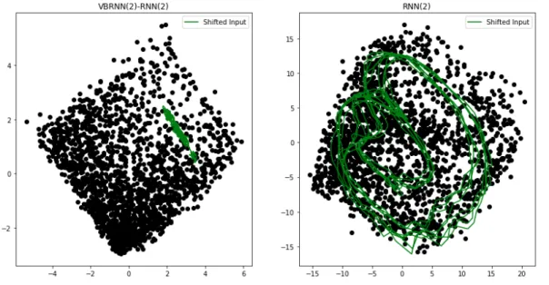
3-8 Timeshifted Trajectory ˜𝑉 for VBRNN(2)-RNN(2) (left) and RNN(2) (right) Trained on Mackey-Glass . . . 52
B-1 Examples of Single Parameter Cosine Dataset . . . 64
B-2 Examples of 2 Parameter Cosine Dataset . . . 65
B-3 Examples of Van der Pol Dataset . . . 66
B-4 Examples of Mackey-Glass Dataset . . . 67
B-5 Graphical Illustration of RNN(1) Latent State for VDP . . . 68
B-6 Graphical Illustration of RNN(2) Latent State for VDP . . . 69
B-7 Graphical Illustration of VBRNN(1)-RNN(1) Latent State for VDP . 70 B-8 Graphical Illustration of VBRNN(2)-RNN(2) Latent State for VDP . 71 B-9 Graphical Illustration of AE Latent State for VDP . . . 72
B-10 Graphical Illustration of VBRNN(1)-AE Latent State for VDP . . . . 73
B-12 Graphical Illustration of VBRNN(2)-DIRECT Latent State for VDP 75 B-13 Graphical Illustration of RNN(1) Latent State for MG . . . 76 B-14 Graphical Illustration of RNN(2) Latent State for MG . . . 77 B-15 Graphical Illustration of VBRNN(1)-RNN(1) Latent State for MG . . 78 B-16 Graphical Illustration of VBRNN(2)-RNN(2) Latent State for MG . . 79 B-17 Graphical Illustration of AE Latent State for MG . . . 80 B-18 Graphical Illustration of VBRNN(1)-AE Latent State for MG . . . . 81 B-19 Graphical Illustration of VBRNN(2)-AE Latent State for MG . . . . 82 B-20 Graphical Illustration of VBRNN(2)-DIRECT Latent State for MG . 83
List of Tables
3.1 Log-Likelihood Model Comparison . . . 36
3.2 The Range of Hyper parameters Tested . . . 40
3.3 Comparison of LSTM and GRU: average log-likelihood in test set . . 41
3.4 𝑅2 for Models of One-Layer Recovery of Generating Parameters for VDP 46 3.5 𝑅2 for Models of Two-Layer Recovery of Generating Parameters for VDP 46 3.6 𝑅2 for Models of One-Layer Recovery of Generating Parameters for MG 46 3.7 𝑅2 for Models of Two-Layer Recovery of Generating Parameters for MG 47 3.8 VDP Clustered Dataset 1 . . . 47
A.1 Conditioning Autoencoder Hyperparameters . . . 60
A.2 Conditioning RNN Hyperparameters . . . 61
Chapter 1
Introduction
Disentanglement in the context of machine learning is a technique used in unsuper-vised learning wherein different features of the underlying problem are inferred and encoded in different dimensions or subgroups within internal state. For example, when learning how to model human faces, a machine learning algorithm might learn to model the gender separate from facial features such as birthmarks. In this context disentanglement makes sense because the gender feature is presumed to be orthogonal to facial features. In many cases perfect disentanglement may not be possible, for ex-ample when distinct features are correlated such as with gender and hairstyle. In this case perfect disentanglement may not be achieved, though the internal representation of such features may still achieve as much separation as possible.
Chapter 1 describes the motivations and background for the thesis, describing in particular other approaches to disentanglement. Emphasis is placed on prior attempts at disentanglement of time constant and time varied features as is demonstrated in this thesis. Chapter 2 introduces the structural components used to force disentan-glement: the Variational Bayes (VB) layer responsible for extracting time constant features, as well as the conditonal-RNN used to model the time dependent dynamics. Additionally, the combination of both are theoretically linked to form the basis of the combined Variational Bayes Recurrent Neural Network (VBRNN). The VBRNN is evaluated in Chapter 3 through the use of model synthetic datasets constructed to explore the various abilities of the model. Finally, Chapter 4 summarizes the
con-tributions of the thesis, and details potential future work to continue exploring the VBRNN and its potential uses with respect to real world problems and applications.
1.1
Motivations for Disentanglement in Time Series
Analysis
Time series in general pose difficulty in modelling due to the added dimension of time, through which additional complex dependencies may manifest. This leads to a natural potential disentanglement, into features that are time dependent, and those that are not (i.e., are time constant or time independent). In general, this factorization makes intuitive sense. Consider two prototypical time series: dynamic systems such as manufacturing processes and biological data such as ECG data representing the electrical potential of heartbeats. In the former case, we expect that the current state of the system is time dependent, depending on where an in-process part is and its current condition, what type of part is being made, and the steps used to make the part. Similarly in the latter case of ECG data, there is easily identifiable time dependent state such as duration and strength of the current heartbeat. The overall shape of any normal heartbeat is the same, however, and this should be time independent. These examples illustrate that, at least at a high level, time dependence is a reasonable condition by which to disentangle time series features; however, it does not address the potential benefit of doing so.
There are two main advantages to performing the disentanglement as described, one in general and one specific to time series. First is the potential ability to extract more information out of a given dataset by way of imposing structure on the problem, and second is the potential to utilize more data in the process of training the model. Imposing structure on a machine learning problem introduces biases and thus narrows and guides the possible space of hypotheses that must be searched. The common consensus is that this makes learning easier as well as improving data ef-ficiency, or how well the training data is used to learn the underlying problem [9].
For example, imposing that a one dimensional regression problem with one input and one output is linear means that a learning algorithm is only tasked with learning the intercept and slope. All of the training data can then be used to learn these two parameters, as opposed to some portion of the data being implicitly used to identify whether the regression is linear, quadratic, or any number of other potential shapes. The downside of adding structure is that imposing incorrect structure can decrease the performance of a model, and care must be taken to verify assumptions implicit to the choice of structure. For disentanglement, however, this is of minimal concern as it is likely that most problems have some form of independent generative factors, under some potentially complex feature transformation. Mathematically, for a linear system, as long as the covariance matrix of the generative factors is non-singular, then the matrix is positive definite and thus diagonalizable. This ensures that the system can be disentangled. This concept can be extended to nonlinear systems with some nonlinear transformation after linearly generated factors.
By disentangling time constant and time dependent features, theoretically more data can be used to train a model. Consider a common problem in time series modelling, nonstationarity. Nonstationarity in a time series is when statistical or mathematical properties, such as the mean, covariance structure or characteristic shape are dependent on time. An example of this contrast would be the time series 𝑥(𝑡) = 𝐶𝑜𝑠(𝑡) versus 𝑥(𝑡) = 𝑓 (𝑡)𝐶𝑜𝑠(𝑡) for some complex function 𝑓 (𝑡). In the latter case, the amplitude envelope of the cosine wave is time dependent, whereas the cosine component is periodic. A machine learning algorithm trained on time 0 < 𝑡 < 10, for example, can be expected to have trouble predicting 𝑡 > 10, as later points in the time series exhibit behavior not seen in the training set, unless 𝑓 (𝑡) were implicitly learned. Learning this implicit problem is expected to be harder, as it manifests at a higher level. To mitigate this, nonstationary time series of this sort would traditionally need to be trained on only data at the end of the training set, say 9 < 𝑡 < 10, and could only be reliably used to predict times close to this reduced training set, say 10 < 𝑡 < 11 under the assumption that 𝑓 (𝑡) is sufficiently smooth and 𝑓 (9) ≈ 𝑓 (10) ≈ 𝑓 (11). Adding explicit structure also gets around this problem as
it forces the model to learn the nonstationary component of the time series. Thus, the entire training set could be used as opposed to a subset, leading to a better learned representation.
Adding structure of this type allows more than just nonstationary data to be used. It also allows families of time series to be learned. Consider some manufacturing process that is subject to a recipe. The underlying dynamics may be the same between runs with different recipes, yet the differences in recipe may cause drastically different outcomes, and thus may pose a problem for a machine learning algorithm. One workaround is to train different models on different runs of the recipe, yet this does not make use of information encoded in runs on other recipes and thus inefficiently uses the given data. A simple model trained on all of the different recipes, however, may perform poorly for any specific recipe, as it only learns to model low order features while missing high order features that are dependent on the specific recipe used. Imposing the disentangled structure thus forces a model to learn these high order components, potentially improving performance across all recipes and thus increasing the efficiency of the model with respect to the data used.
1.2
Related Works
Disentanglement is not a new concept. Many authors have demonstrated disentan-glement of various forms [5][3], as well as the benefits of disentandisentan-glement [13][10][4]. Specifically, there are a few works worth highlighting in the context of this thesis.
In introducting the 𝛽-𝑣𝑎𝑒, Higgins et al. [6] demonstrate disentanglement in variational autoencoders. They use a variant of an autoencoder (described in more detail in Section 2.3.1) where the output of the encoder is a probabilistic distribution across encodings instead of a direct encoding. Training this model now adds a term to quantify the difference between the posterior encodings and the prior, akin to what is done in Section 2.2.2 through the use of a KL-divergence term. They show that increasing the constant on the KL-divergence term between the posterior and prior causes a marked increase in the disentanglement of the learned encoding, as shown
through various image reconstruction tasks. This is significant as it demonstrates that adjusting the coefficient of a training metric has a significant impact in the demonstrated disentanglement of an unsupervised model.
Kumar et al. present a model similar in function to the 𝛽-𝑣𝑎𝑒 which disentangles using variation inference via the addition of a regularizer over the inferred posterior to coerce a more diagonal covariance matrix [9]. They demonstrate empirically better performance, as well as a new disentanglement metric called Separated Attribute Pre-dictability, or SAP, which seeks to explicitly quantify disentanglement by examining the effect on the output of individual encoding dimensions.
Kingma et al. demonstrate effective variational Bayesian inference, upon which the time constant feature estimation is based [8]. They do this with careful construc-tion of an approximate lower bound to mitigate the intractable posterior, which is a trick used with the proposed approach.
Chung et al. introduced the VRNN, or variational recurrent neural network, which disentangles the deterministic and stochastic hidden state of a model [2]. This represents a somewhat similar approach as presented in this thesis, albeit to perform a different type of disentanglement. Their approach largely inspired the proposed approach, and is thus discussed in more detail in the theoretical derivation portion of Chapter 2.
Building off of the VRNN, Yingzhen and Mandt proposed disentangling the hid-den state further [11], akin to the intent of this thesis. They proposed encoding time constant hidden state apart from time varying hidden state, allowing for more powerful generative models. Their overall approach is not explicitly defined, though they mention structurally disentangling hidden state by constraining the size of the hidden states 𝐻 and 𝑌 in a model similar to the VRNN. Empirically, they were able to change the gender of speech samples, and change the appearance of sprites in animations.
Figure 1-1: An example of an autoencoder-conditioned VBRNN
1.3
General Model Overview
The proposed VBRNN model is composed of three distinct components. First, a feature extractor is used for dimensionality reduction, then a variational Bayes layer extracts an approximate posterior of the time constant features, and finally the pos-terior is sampled and used to condition an RNN. Here we give an overview of the various parts of the model; for a more technical description see the theoretical for-mulation of the problem in Section 2.2. An example of the overall structure is shown schematically in Figure 1-1, here an autoencoder is used for dimensionality reduc-tion, and an additional feature extractor is used after the variational inference block to conditioned the RNN.
In the general VBRNN structure, the first component is an unsupervised feature extractor for the purposes of dimensionality reduction. In practice this can take many forms, but the two explored approaches in this thesis are with an autoencoder and with an RNN model. Both are trained on the data in an unsupervised manner until sufficient modelling ability is achieved. The hidden state of the autoencoder, or the final hidden state of the RNN, are used as the output of this component. We expect that these extracted features encode all the necessary information about time constant features in some lower dimensionality than the input. This component is not strictly necessary, however, and can be skipped by providing the input directly to the variational Bayes layer. Research shows, though, that unsupervised feature
extraction can improve existing models, as demonstrated by Ren et al. [12]. This component or layer can be trained separately from the rest of the model, and this is done for all the experiments performed in this thesis.
The second component is the variational Bayes layer. This layer takes input from the previous, and outputs an approximate independent Gaussian posterior in the form of a mean and standard deviation vector. This layer is trained with a KL-divergence term between the approximate posterior and some predefined prior, generally a standard normal. The output is then sampled from this posterior for training, or the mean is used for model evaluation.
Finally, the sampled posterior is used to condition a standard RNN model in the last component. This can be done in one of two ways. Either the entire extracted posterior can be concatenated with the input to every RNN layer (recurrence layers and prediction layer), or a single layer feature extractor can be used to extract a different set of conditioning variables per RNN layer. For the experiments performed in this thesis the latter is used, as extracting different conditioning variables per layer potentially yields some extra interpretability.
Chapter 2
Theory
The theory that the VBRNN is built upon is well established; it uses the same ground-work as the original RNN. This chapter begins with an overview of the necessary theoretical foundations, and then presents a description of the problem. This chap-ter finishes with a presentation of the training algorithm for the proposed VBRNN model.
2.1
Prior Related Theory
We begin with a brief review of related theory leading up to the theoretical formula-tion of the VBRNN model. Most machine learning time series modelling approaches involve hidden state, where there is assumed to be some unobservable or hidden state 𝑍𝑡at every time step which influences observations 𝑌𝑡. This gives rise to the following
learned factorized distribution:
𝑃 (𝑌1:𝑇, 𝑍1:𝑇) = 𝑇
∏︁
𝑖=1
𝑃 (𝑌𝑡≤𝑖|𝑍𝑡≤𝑖)𝑃 (𝑍𝑡≤𝑖). (2.1)
In theory, this is capable of modelling any time series with dependencies over any time scale. For example, when modelling a sentence, any word in the text could have a relationship to any other preceding or following word arbitrarily far away. In a man-ufacturing context, a sensor observation for a tool could be correlated with the first
observations ever made on the tool post its construction. While theoretically sound, the dimensionality of this distribution grows with the size of the input, realistically limiting the types of models that can be learned. RNNs traditionally have fixed sized hidden state ℎ, but mitigate this by learning a recurrence function 𝑓 that transitions ℎ over time given observations 𝑋𝑡. Coupled with an observation model 𝑔, RNNs with
limited state size approximate the aforementioned distribution as
𝑃 (𝑌1:𝑇, 𝑍1:𝑇) ∝∼ 𝑔(ℎ𝑡), (2.2)
ℎ𝑡+1 = 𝑓 (ℎ𝑡, 𝑦𝑡). (2.3)
As the size of ℎ grows, theoretically an RNN can learn any time series distribu-tion. The challenge for realistically sized hidden state, however, is that the transition function 𝑓 must be sufficiently complex to maintain any relevant information about arbitrarily distant prior observations. In the manufacturing example with a tool, the hidden state likely must implicitly encode information about the calibration of the tool or import characteristics of its construction time series. It must also encode in-formation about the wear of the device, which can be assumed to be slowly changing over time. Historically this difficulty has led to the vanishing gradient problem, where learning to maintain information about distant time steps has arbitrarily small gradi-ents and is thus incapable of being learned. More recent approaches have introduced the concept of memory [7]. The classic example is the LSTM, or Long-Short Term Memory. LSTMs introduce two important additions to the standard RNN. First is a forget gate. This gate controls how information is “forgotten” with the hidden state ℎ to make room for information from new observations. Second is the accompanying hidden state 𝑐, which encodes information about how the forget gate should operate. Loosely, the functioning of an LSTM can be written as follows:
𝑃 (𝑌1:𝑇, 𝑍1:𝑇) ∝∼ 𝑔(ℎ𝑡), (2.4)
𝑐𝑡+1 = 𝑓𝑐(ℎ𝑡, 𝑐𝑡, 𝑦𝑡). (2.6)
This represents a basic form of disentanglement, where hidden state is structurally partitioned into states that encode information about different parts of the process. For LSTMs, ℎ encodes relevant information about prior states, whereas 𝑐 encodes information about how ℎ should evolve over time. This greatly improved the perfor-mance of RNNs on both synthetic and real world data, and enabled a much richer set of models to be learned for a variety of tasks [14].
Another problem that appears, however, is the deterministic nature of RNNs. In the formulation for both the standard RNN and LSTMs, transition functions 𝑓 are deterministic: given an 𝑓 and 𝑌1:𝑇 the evolution of the ℎ are purely deterministic.
As with previous problems, as ℎ grows larger and the observation model 𝑔 grows more complex, any distribution can be learned. Again in practice, constraining any stochastic variability in a time series purely through the observation model requires increasingly complex 𝑔. To mitigate this problem, Chung et al. introduced the VRNN or Variational Recurrent Neural Network [2]. The VRNN model introduces a second hidden state 𝑋 that encodes stochastic latent variables that are generated using the variational autoencoder for inferencing purposes. In this model, hidden state ℎ is used to generate a distribution on 𝑋. Per time step, this distribution is randomly sampled to get 𝑥, which is then used in the observation model. Building off a standard RNN (though an LSTM can be used, for example), the formulation is as follows:
𝑃 (𝑥𝑡|ℎ𝑡) = 𝑓𝑥(ℎ𝑡), (2.7)
𝑃 (𝑌1:𝑇, 𝑋1:𝑇) ∝∼ 𝑔(ℎ𝑡, 𝑥𝑡), (2.8)
ℎ𝑡+1= 𝑓 (ℎ𝑡, 𝑦𝑡, 𝑥𝑡). (2.9)
𝑃 (𝑥𝑡|𝑦𝑡ℎ𝑡) ≈ 𝑞(ℎ𝑡, 𝑦𝑡). (2.10)
Typically, the distribution across 𝑋 is constrained to be gaussian; the model 𝑓𝑥
𝑋. This distribution is then sampled to get 𝑥𝑡, then is fed into the observation
model with ℎ𝑡 to generate the prediction for 𝑦𝑡. The actual 𝑦𝑡 is fed into the encoder
𝑞(ℎ𝑡, 𝑦𝑡) generating an approximate posterior which can then be compared against
the generated prior distribution. This enables the use of the variational lower bound
log 𝑝(𝑦𝑡) ≥ −𝐾𝐿(𝑃 (𝑥𝑡|ℎ𝑡)||𝑃 (𝑥𝑡|𝑦𝑡, ℎ𝑡) + 𝐸𝑔(𝑦𝑡|ℎ𝑡,𝑥𝑡)[log 𝑝(𝑦𝑡|ℎ𝑡, 𝑥𝑡)]. (2.11)
This formula bounds the log likelihood of 𝑦𝑡 with the KL divergence between the
prior and posterior as well as the expected log likelihood of the prediction. Since the posterior is intractable, it is impossible to explicitly evaluate the first term. This is why we instead define the prior in terms of 𝑓𝑥(ℎ𝑡), and the approximate posterior
𝑞(ℎ𝑡, 𝑦𝑡) which attempts to learn the inverse of 𝑓𝑥(ℎ𝑡). Thus we approximate the first
term as 𝐾𝐿(𝑓𝑥(𝑥𝑡|ℎ𝑡)||𝑞(𝑥𝑡|𝑦𝑡, ℎ𝑡). The second term represents the expectation across
the prior distribution of 𝑋 of our prediction of 𝑌 , which is Monte-Carlo estimated through our sampling of 𝑋. The VRNN represents another step in disentangling hidden state, between stochastic and deterministic hidden state. This allows more complex models for a given size hidden state, and is empirically shown to be better at modelling speech patterns [2]. This differs in the type of hidden state that is disentangled, yet represents a similar approach to the VBRNN presented in this thesis both in structure and theory.
2.2
Problem Description
This section and the following definition of the problem we are seeking to solve are heavily based on a note formalizing discussions about the problem and approach as presented by my collaborator Kyongmin Yeo at IBM.
2.2.1
Generation of 𝑌
Prior, we discussed modelling some time series 𝑌1:𝑇. Yet here it is useful to describe
physical state of the system, governed by a system of possibly nonlinear differential equations with parameters 𝜋 ∈ 𝑅𝑁𝜋:
𝑑𝜇
𝑑𝑡 = 𝐹 (𝜇; 𝜋). (2.12)
We assume, however, that 𝜇 is unobservable, and thus we can only observe 𝑌 which has some inherent observational noise 𝜖.
𝑦𝑡 = 𝜇𝑡+ 𝜖𝑡. (2.13)
Furthermore, we assume that 𝜋 is a random variable with some (potentially unknown) probability distribution 𝑝(𝜋). Thus the complete generating distribution is
𝑝(𝑌1:𝑇, 𝜋) = 𝑝(𝑌1:𝑇|𝜋)𝑝(𝜋). (2.14)
2.2.2
Inference of 𝜋
For the purposes of disentanglement, we wish to infer 𝜋 separately from our modelling of 𝑌 . Direct inference of 𝜋 is impossible without prior knowledge of 𝐹 (𝜇; 𝜋). We can, however, assume some latent variable 𝑣 that allows an approximation of the data generating distribution:
𝑝(𝑌1:𝑇, 𝜋) ≈ 𝑝(𝑌1:𝑇|𝑣)𝑝(𝑣). (2.15)
Instead of attempting to infer 𝜋 we instead infer 𝑣. An additional difficulty is pre-sented by the fact that the posterior distribution of 𝑣, 𝑝(𝑣|𝑌1:𝑡) is inaccessible;
in-stead we learn some approximate posterior distribution 𝑞(𝑣|𝑌1:𝑡). In order to simplify
the model, we assume that the output of 𝑞 is a normal with diagonal covariance 𝒩 (𝜇𝑞, 𝑑𝑖𝑎𝑔(𝜎2𝑞)) for some outputs 𝜇𝑞, 𝑑𝑖𝑎𝑔(𝜎𝑞2) as learned by a neural network 𝜈.
Ad-ditionally, we assume the prior 𝑝(𝑣) is also a normal distribution with zero mean and diagonal covariance 𝒩 (0, 𝜎𝑣2𝐼). When training 𝜈 to learn 𝑞, we can use the Knullback-Leibler divergence to characterize the difference between the prior 𝑝(𝑣) and our approximated posterior 𝑞(𝑣|𝑌1:𝑡). Since we constrain both our posterior and
prior to be gaussians with diagonal covariance, we know that 𝐷𝐾𝐿(𝑞(𝑣|𝑌1:𝑡)||𝑝(𝑣)) = 𝑁𝑣 ∑︁ 𝑖=1 {︂1 2 𝜎2 𝑞𝑖+ 𝜇𝑞𝑖 𝜎2 𝑣 − 𝑙𝑜𝑔 (︂𝜎 𝑞𝑖 𝜎𝑣 )︂}︂ − 𝑁𝑣 2 (2.16)
2.2.3
Modelling 𝑌
Once we have a posterior for 𝑣, we can use a conditional RNN to model 𝑌 . For a normal RNN modelling 𝑃 (𝑌𝑡|𝑌1:𝑡) we have the recurrence relation
ℎ𝑛= Ψ(ℎ𝑡−1, 𝑦𝑡−1) (2.17)
𝑃 (𝑌𝑡|𝑌1:𝑡) = 𝜑(ℎ𝑛) (2.18)
for state transition function Ψ and prediction function 𝜑. Of course, we are not trying to model 𝑃 (𝑌𝑡|𝑌1:𝑡), but rather 𝑃 (𝑌𝑡|𝑌1:𝑡, 𝑣). If we assume that we have 𝑣, we can
model this by similarly conditioning both functions to give us a conditional RNN
ℎ𝑛= Ψ(ℎ𝑡−1, 𝑦𝑡−1, 𝑣) (2.19)
𝑃 (𝑌𝑡|𝑌1:𝑡, 𝑣) = 𝜑(ℎ𝑛, 𝑣). (2.20)
Next, to get back to 𝑃 (𝑌𝑡|𝑌1:𝑡) we must marginalize out 𝑣. Since we do not have 𝑣
explicitly but rather 𝑞(𝑣|𝑌1:𝑡) as derived in the previous section, in order to marginalize
out 𝑣 we must use
𝑃 (𝑌𝑡|𝑌1:𝑡) =
∫︁
𝑣
𝑃 (𝑌𝑡|𝑌1:𝑡, 𝑣)𝑝(𝑣|𝑌𝑡:𝑡)𝑑𝑣. (2.21)
Since this integral is intractable, we can Monte Carlo estimate this integral by repeat-edly sampling 𝑣, performing our prediction with the sampled 𝑣, then averaging across all the predictions. Now since 𝜑 outputs a predictive distribution, we again constrain the distribution to be normal gaussian with diagonal covariance. The output of 𝜑 is then 𝜇𝜑𝑡, 𝜎
2
𝜑𝑡 which represents 𝒩 (𝜇𝜑𝑡, 𝑑𝑖𝑎𝑔(𝜎
2
sampling of 𝑣) is then given by ∑︁ 𝑡 𝑁𝑦 ∑︁ 𝑖=1 1 2 (𝑦𝑡𝑖 − 𝜇𝜑𝑡𝑖) 2 𝜎2 𝜑𝑡𝑖 + 𝑙𝑜𝑔(𝜎𝜑𝑡𝑖). (2.22)
Of course, the overall loss must be sampled from 𝑣 as described, so the overall recon-struction loss is ℒ𝑦 = 𝐸𝑞 [︂ ∑︁ 𝑡 𝑁𝑦 ∑︁ 𝑖=1 1 2 (𝑦𝑡𝑖 − 𝜇𝜑𝑡𝑖) 2 𝜎2 𝜑𝑡𝑖 + 𝑙𝑜𝑔(𝜎𝜑𝑡𝑖) ]︂ . (2.23)
2.3
Training of the VBRNN
Training of the VBRNN occurs in two steps. First, an unsupervised feature extractor is trained, then these extracted features are used to train the rest of the VBRNN. This process consists of training the variational Bayes layer in combination with the conditioned RNN by combining their respective loss functions.
2.3.1
Unsupervised Feature Extraction
There are multiple choices of feature extractor; the two used in this thesis are an autoencoder and an RNN. Other dimensionality reduction and feature extraction techniques could be used, however.
Autoencoder Training
An autoencoder simply learns some function 𝑓 as well as its approximate inverse 𝑔 such that for a given input 𝑥, 𝑔(𝑓 (𝑥)) ≈ 𝑥. Generally the dimensionality of the output of 𝑓 is constrained to be smaller than the input such that 𝑓 (𝑥) encodes 𝑥 in some lower dimension. This is useful for both learning compressed encodings as well for unsupervised feature extraction. Additionally, the size of the input is also fixed in size, so when used with variable length time series, a fixed sized window sampled from a time series must be used. See Appendix A for the hyperparameters used to train the models. To train an autoencoder of input size 𝑁𝐴 given the aformentioned dataset 𝐷
some number of trajectories proportional to the batch size, then for each trajectory subsample 𝑁𝐴 time steps. Each of these samples is then vertically concatenated to
form a single batch over which the autoencoder is trained as a standard feedforward neural net. For a given batch 𝑏, loss is defined as
ℒ𝑎𝑢𝑡𝑜𝑒𝑛𝑐𝑜𝑑𝑒𝑟 = 𝑀 𝑆𝐸(𝑏, 𝑔(𝑓 (𝑥)) (2.24)
for standard mean squared error under the assumption that the errors are normally distributed. The extracted features per batch are the output of the encoding layer 𝑓 (𝑥).
RNN Training
Training the RNN is very similar to training the autoencoder. The two main differ-ences are that an RNN can take in variable length input sequdiffer-ences, and in our usage makes single step predictions. Since we will seek to compare the effect of conditioning a VBRNN with an RNN, to conditioning a VBRNN with an autoencoder, we wish to have the models as comparable as possible. To do this, we generate batches equiva-lently to training the autoencoder such that the RNN learns to extract information from an identically sized input window. Loss for a given output 𝑅𝑁 𝑁 (𝑏) for batch 𝑏 is similarly defined as
ℒ𝑅𝑁 𝑁 = 𝑀 𝑆𝐸(𝑏:,1:𝑁𝐴, 𝑅𝑁 𝑁 (𝑏):,0:𝑁𝐴−1) (2.25)
with single time step offsets to account for the one-step predictions of the RNN. The extracted features are then taken as the final hidden layer of the RNN.
2.3.2
Training Variational Bayes and RNN
Training the VBRNN is akin to training a standard conditional RNN. The only dif-ference is that to force disentanglement, we extract time constant features 𝑣 from an independent sample of the time series. Thus when generating a batch for training,
we perform a two step process to generate two related batches for different sections of the time series. Similar to the training of the feature extractors, we first select 𝑁𝑏
trajectories (with replacement). Again, see Appendix A for specific hyperparameters used for the given tests. Then, from each trajectory we subsample a fixed 𝑁𝐴 sized
window. These are concatenated vertically to form 𝑏𝑣. Next, from each trajectory we again independently subsample an 𝑁𝑅𝑁 𝑁 sized window to train the later RNN
portion of the VBRNN. Vertically concatenating these forms 𝑏𝑅𝑁 𝑁. In this way 𝑏𝑣 and 𝑏𝑅𝑁 𝑁 contain samples from the same trajectories but from potentially different
windows within the trajectory. This difference in sample location nudges the varia-tional Bayes layer to only extract information of a time constant nature as desired, and empirically showed better performance during the development process of the model, though explicit results are not presented in this thesis. To train the model, 𝑏𝑣 is passed through the feature extractor of choice, then through the variational Bayes layer and sampled as described in Section 2.2.2 to get 𝑣, with associated loss 𝐷𝐾𝐿(𝑞(𝑣|𝑌1:𝑡)||𝑝(𝑣)). This is then horizontally concatenated with every datapoint in
𝑏𝑅𝑁 𝑁 to form the conditioned input, and fed into the 𝑅𝑁 𝑁 layer as described in
Section 2.2.3 with associated loss ℒ𝑦. Overall the loss then becomes
ℒ = 𝐷𝐾𝐿(𝑞(𝑣|𝑌1:𝑡)||𝑝(𝑣)) + ℒ𝑦 (2.26)
per batch. Standard backpropagation is then performed to train the RNN and vari-ational Bayes layers jointly, with the feature extractor layers frozen.
Chapter 3
Experimental Results
Overall the premise of the VBRNN is relatively straighforward: to disentangle time constant and time dependent hidden state. Empirically evaluating the effectiveness of this model is more difficult. To best explore the practical capabilities of the VBRNN, multiple experiments are performed over a variety of different synthetic datasets. The chapter begins with a description of the specific datasets used, followed by discussion of experiments into the model overall. Finally, experiments diving more deeply into the latent space of encodings produced by the model are presented.
3.1
Datasets
In order to best explore the potential of the VBRNN, multiple synthetic datasets are generated to test the VBRNN in an controlled manner. Below are the selected datasets in order of complexity. See Appendix B for graphed examples of the various datasets.
3.1.1
Single Parameter Cosine Wave
The single parameter cosine wave dataset represents a simple nonlinear time series with latent parameters suitable for exploration of the VBRNN. The dataset is
com-prised of 500 trajectories of 1000 time steps, each generated according to the following: 𝑦(𝑡) = 0.5 + 0.5 · 𝐴 · 𝑐𝑜𝑠((𝑡 + 𝑦0) ·2𝜋𝑇 ) ˜ 𝑦(𝑡) = 𝑦(𝑡) + 𝜖𝑡, 𝜖𝑡∼ 𝒩 (0, 0.05) 𝐴 ∼ 𝒰 (0.1, 1) 𝑦0 ∼ 𝒰 (0, 100) 𝑇 = 100 (3.1)
where 𝒰 (0, 100) represents a uniform distribution in the interval (𝑎, 𝑏].
The data is then stored as a noiseless time series, a noisy time series, and the sampled parameters. For this dataset the added noise for the noisy time series is gaussian with constant variance of 0.05.
The single parameter cosine wave has two latent parameters, the amplitude and the starting position. However, the starting position is fundamentally inseparable from time dependent features (namely position) and thus is not considered when attempting to recover the latent parameters.
3.1.2
Two Parameter Cosine Wave
The two parameter cosine wave dataset represents a slightly more difficult nonlinear time series than the single parameter cosine wave, with the introduction of a latently sampled period. The dataset is similarly comprised of 500 trajectories of 1000 time steps, each now generated according to the following:
𝑦(𝑡) = 0.5 + 0.5 · 𝐴 · 𝑐𝑜𝑠((𝑡 + 𝑦0) ·2𝜋𝑇 ) ˜ 𝑦(𝑡) = 𝑦(𝑡) + 𝜖𝑡, 𝜖𝑡∼ 𝒩 (0, 0.05) 𝐴 ∼ 𝒰 (0.1, 1) 𝑇 ∼ 𝒰 (50, 200) 𝑦0 ∼ 𝒰 (0, 2 · 𝑇 ) (3.2)
The data is again stored as a noiseless time series, a noisy time series, and the sampled parameters. For this dataset the added noise is gaussian with constant variance 0.05.
Similarly to the previous dataset, the two parameter cosine wave actually has three latent parameters, the amplitude, period, and the starting position. Akin to the single parameter cosine wave, the starting position is fundamentally inseparable and thus is not considered a time constant feature.
3.1.3
Forced Van der Pol Oscillator
The forced Van der Pol oscillator represents another step up in complexity, and is generated from a nonlinear second order ODE. The dataset is comprised of 2000 trajectories of 1000 time steps each, generated according to the following:
𝑑2𝑦 𝑑𝑡2 = 𝛼(1 − 𝑦 2)𝑑𝑦 𝑑𝑡 = 𝑦 + 𝐴𝑠𝑖𝑛( 2𝜋 𝜏 𝑡) ˜ 𝑦(𝑡) = 𝑦(𝑡) + 𝜖𝑡, 𝜖𝑡 ∼ 𝒩 (0, 𝜎2) 𝛼 ∼ 𝒰 (4, 10) 𝐴 ∼ 𝒰 (1, 10) 𝜏 ∼ 𝒰 (1, 30) 𝜎2 ∼ 𝒰 (0.05, 0.1) (3.3)
The data is also stored as a noiseless time series, a noisy time series, and the sampled parameters. For this dataset, the added noise is gaussian with a latently sampled variance between 0.05 and 0.1. Thus there are four latent parameters that affect the shape of the oscillator, the shape of the forcing sine wave, and the observational noise.
3.1.4
Clustered Forced Van der Pol Oscillator
For the purposes of testing the ability of the VBRNN to cluster parameters in the recovered latent space, artificial clusters in the parameter space are created for the clustered forced Van der Pol oscillator datasets. See Section 3.3.3 for experimental details. For different experiments, different clusters are arranged, and are detailed in the respective sections. For a given point in a given cluster, parameters are sampled
Figure 3-1: The effect of small changes to 𝜏 for Mackey Glass
according to the cluster distribution, and then sampled as before from
𝑑2𝑦 𝑑𝑡2 = 𝛼(1 − 𝑦 2)𝑑𝑦 𝑑𝑡 = 𝑦 + 𝐴𝑠𝑖𝑛( 2𝜋 𝜏 𝑡) ˜ 𝑦(𝑡) = 𝑦(𝑡) + 𝜖𝑡, 𝜖𝑡 ∝ 𝒩 (0, 𝜎2). (3.4)
3.1.5
Chaotic Mackey-Glass Time Series
As a final step up in complexity, a chaotoic Mackey-Glass time series is used. With only a single latently sampled parameter (not including fixed parameters, initial con-ditions or added noise) the latent space is relatively simple, yet slight changes in parameters have large effects on the time series trajectories, as seen in Fig. 3-1.
The dataset is comprised of 2000 trajectories of 1000 time steps each, generated according to 𝑑𝑦 𝑑𝑡 = 𝛼𝑦(𝑡−𝜏 ) 1+𝑦𝛽(𝑡−𝜏 ) − 𝛾𝑦 ˜ 𝑦(𝑡) = 𝑦(𝑡) + 𝜖𝑡, 𝜖𝑡 ∼ 𝒩 (0, 𝜎2) 𝜏 ∼ 𝒰 (16, 40) 𝜎2 ∼ 𝒰 (0.05, 0.1) 𝛼 = 0.2 𝛽 = 0.1 𝛾 = 10 (3.5)
The constants 𝛼, 𝛽, 𝛾 are known to cause the Mackey-Glass time series to be chaotic.
3.2
General Model Exploration
Here we present a set of experiments to explore the general performance of the VBRNN and its variants as compared to an RNN, in both single and multistep predictions. We also discuss key considerations when training the VBRNN, such as sensitivity to choice of hyperparemeters.
3.2.1
Model Training Performance
As detailed in Section 2.3, the core of the VBRNN is trained with single-step log-likelihood (LL) as the reconstruction loss. Performance with respect to this loss metric allows a basic and easy preliminary comparison of models. Since the single-step LL is used by both the RNN and VBRNN models, it also allows direct comparisons between the two. Of course, we also train the VRBNN with respect to the KL divergence; however, this loss is mostly noninformative as divergence from the prior does not directly tell us how well the model will perform in out of sample prediction performance. Rather, the KD divergence gives insight into how much information is contained within the latent encoding, though this may not directly correspond to model performance with respect to time predictions [1].
For this experiment, models are trained on the two parameter cosine wave dataset detailed in Section 3.1.2, the forced Van der Pol oscillator dataset detailed in Sec-tion 3.1.3 and the Mackey-Glass dataset detailed in SecSec-tion 3.1.5, hereafter referred to as COS, VDP, and MG datasets, respectively. These datasets are selected as they are all relatively straightforward with no complications such as clustered parameters, and are thus good candidates to explore overall model performance. Models are trained according to the hyper parameters in Appendix A. Each 2000 trajectory dataset is split into 1600/200/200 train/test/validation splits. Approximately 20 models are trained for each model variant per dataset, and the best model is selected via the test split. Models are then compared on performance in the validation split as indicated
Table 3.1: Log-Likelihood Model Comparison Model Cos VDP MG RNN(1) 1057.21 1269.67 1330.24 RNN(2) / 1301.03 1370.86 VBRNN(1)-RNN(1) 1064.82 1300.70 1380.76 VBRNN(2)-RNN(2) / 1311.60 1400.60 VBRNN(1)-AE 1061.32 1318.32 1405.34 VBRNN(2)-AE / 1327.91 1413.56 VBRNN(2)-DIRECT / 1316.58 1383.96
by the single-step LL reconstruction error. Results are shown in Table 3.1.
In Table 3.1 (and in subsequent discussion), the following notation is used: RNN(1) and RNN(2) refer to one-stage and two-stage RNNs, respectively. Similarly VBRNN(1) and VBRNN(2) refer to one-stage and two-stage VBRNN models. Additionally, the type of model used to condition the VBRNN is indicated after a dash; for example, VBRNN(2)-RNN(2) refers to a two stage VBRNN model conditioned on a two-stage RNN model, while VBRNN(2)-DIRECT refers to a two-stage VBRNN conditioned on the underlying time series directly without a conditioning feature extractor.
Overall model performances are highly similar, with at most 6% difference be-tween the best and worst performing models per dataset. Additionally, while not shown, individual runs of each model-dataset pair are generally within a few percent of each other (with outliers on the low end indicating unescaped local minima). Since the spread between individual runs is moderately smaller than the spread between models, this indicates that model-to-model comparison is statistically significant yet not strongly so, and such a small difference should be considered cautiously especially for untested datasets.
For each model where a one-stage and two-stage RNN are tested, the two-stage model outperformed the one-stage model by moderate margins. This is to be expected as both the MG and VDP datasets are highly nonlinear, and the addition of another RNN layer allows for more nonlinearity in modelling.
is a strong positive sign for the VBRNN. Since the VBRNN is based off the RNN, the strong performance indicates that the addition of the variational Bayes layer is having a positive effect with respect to general model performance.
Between conditioning variants of the VBRNN, the picture is less straightforward. For both the more complex VDP and MG datasets, the autoencoder-conditioned VRBNN outperforms the RNN conditioned model. The reverse is true of the COS dataset, however, though the margins are much smaller. Assuming both the condi-tioning autoencoder and RNN encode the same latent information, the larger input from the RNN (128 for RNN(1), 256 for RNN(2) vs. 25 for AE) would potentially cause the VBRNN to overfit more and thus have worse out of sample performance. As is shown in Section 3.3 and 3.3.2, however, the RNN encodes far more informa-tion about the latent parameters and thus the VBRNN-RNN should outperform the VBRNN-AE. This potentially indicates that the RNN-conditioned VBRNN must be more carefully trained, perhaps with steps to avoid overfitting such as dropout or regularization.
In all of the cases in this experiment, the AE outperforms the VBRNN-direct. Since both the encoder and variational Bayes layers (excluding the final) share the same shape (a monotonically shrinking feedforward network), using an autoencoder to condition is structurally equivalent to increasing the depth of the VB layer. This is significant since it means that there is more of a benefit to using the autoencoder than simply adding more layers: the autoencoder has learned more efficient initial layers in an unsupervised fashion.
Overall these results show that all variants of the VBRNN have the potential to outperform the vanilla RNN, and using some form of unsupervised feature extraction is of value. Further exploration is required to see if the VBRNN-RNN can be better trained to overcome potential overfitting issues.
3.2.2
Multistep Predictions Comparison
One potential benefit of disentangling time constant hidden state is that any such unchanging state is explicitly persistent and not subject to vanishing gradients. In
vanilla RNNs, any extracted info about time-constant state would have smaller and smaller gradients with respect to future time steps and thus persisting such state over longer timescales would be learned at a slower rate. Imperfect models would thus lose inferred time constant state with each time step. With the VBRNN, any such constant state disentangled into the conditioning features would be applied equally to all time steps with no information leakage. This would imply that the VBRNN would better be able to make multistep predictions.
To test this potential benefit of the VBRNN, multistep predictions are needed. Since an RNN or VBRNN only gives single step predictions per time step, the models must be run in closed loop mode. To do this, once a multistep prediction is desired, rather than feeding in the next point in the input time series, the output of the previous time step is fed back into the model. Of course, since the output at any time step is a probabilistic distribution, a single point must be sampled before being fed back in. A single run then gives a single sample of the probabilistic multistep prediction. In order to approximate the overall distribution across multiple time steps, this sampling must be done multiple times to estimate the overall distribution. For simplicity of comparison, these Monte Carlo samples are then averaged to get the mean prediction which can then be used to find the mean square error of the multistep predition.
To test basic multistep prediction error, the COS dataset is selected. This is due both to the simplicity and periodic nature of the time series. The Mackey-Glass time series would likely be difficult to compare, as predictions would quickly diverge due to its chaotic nature. Similarly, the VDP oscillator is not perfectly periodic (at least over short timescales) and can have subtle effects due to the forcing; for the purposes of this initial basic experiment we seek to explore performance in ideal circumstances. To setup the experiment, all of the models trained on the COS dataset in Sec-tion 3.2.1 are used to multistep-predict the last 400 time steps of the validaSec-tion trajectories. The MSE per time step is calculated and plotted for each of the RNN, VRNN-RNN, and VRNN-AE models, respectively, in the upper half of Figure 3-2. The black line represents the median MSE across all of the training runs, while the
Figure 3-2: Cosine Multistep Comparison
grey line represents the mean MSE per time step. The bottom plot shows the mean with a dotted line and the median with a solid line, in their respective colors.
The results are immediately clear: both of the VBRNN models outperform the RNN model, with the RNN-conditioned VBRNN significantly outperforming the autoencoder-conditioned one. This is the expected result, and nicely demonstrates the effect of disentanglement on multistep predictions. In addition, this mirrors the results in Section 3.3 and Section 3.3.2 which demonstrate the RNN’s ability to better extract latent time constant features than an autoencoder for the purposes of feature extraction for the VBRNN. Additionally, this shows that good single step performance as in Section 3.2.1 does not necessarily equate to multistep performance.
Table 3.2: The Range of Hyper parameters Tested
Param Min Max
v-dim 6 15 v-height 1 3 c-dim 5 14 RNN dim 64 256 RNN height 1 3
3.2.3
Hyperparameter Study
One key aspect of a model is how sensitive it is to choice of hyperparameters, since this determines how much tuning is necessary to get optimal results. To test this, in this section many models are trained with varying hyperparameters sampled from a random distribution within a reasonable range, as shown in Table 3.2, in addition to randomly selecting between GRU or LSTM cells. This excludes the v-prior hy-perparameter, which is explored in the next section (Section 3.2.4). Here v-dim and v-height refer to the width and height, respectively, of the variational Bayes layer, while c-dim refers to the dimension of the variables used to condition the final RNN layer. The models are trained on truncated versions of the VDP and MG datasets, i.e., with 100 trajectories each in order to facilitate a larger number of hyperparameter samples.
Once trained, the initial check is to see the relative performances of the LSTM and GRU cells. The average log-likelihoods are shown in Table 3.3. For both datasets, GRU models significantly outperform LSTM cells. While the exact reason is not known for sure, it is likely due to the reduced number of parameters in a GRU cell, resulting in better resistance to overfitting. It is possible that the comparatively simpler variatonal Bayes and conditioning layers train faster than the RNN cells, and thus a reduced parameter RNN cell is beneficial. It is also possible that this decreased overfitting is an artifact of the relatively small size of the training datasets. Regardless, the significantly better performance of the GRU cell motivates its selection for training models in other experiments presented here.
Table 3.3: Comparison of LSTM and GRU: average log-likelihood in test set
Dataset LSTM ave LL GRU ave LL
VDP 564.64 626.98
MG 1179.36 1261.25
Next, in order to explore the importance of the other hyperparameters, various regressions are performed in an attempt to map from choice of hyperparameter to model performance. For each dataset, 600 samples of trained models are collected. The first 500 are used to train the regression, with the last 100 left as a test set. Simple linear regressions are used first, but are unable to achieve any predictive power. Next, polynomial regressions of up to order four are tested with again no predictive power in the test set. Next, random forest regressors are used to explore more complex nonlinearities, and again no predictive power is found. The lack of ability of any of these models to find predictive power from the choice of hyperparameters to expected model performance implies that the model is highly insensitive to its hyperparameters. This is a strong positive sign for the VBRNN, as it implies that the model will require minimal to no tuning. Of course, only two relatively small datasets have been explored here and with a moderate number of samples; it is possible that these results do not hold for other datasets or that there may be modest benefit to be had from some minor tuning. However, the observed lack of dependence on hyperparameters is another positive result for the VBRNN.
3.2.4
V-Prior Study
Theoretically, the choice of prior for the variational Bayes layer (referred to here as v-prior) should not matter for the given formulation and training routine. This is due to the fact that the sampled extracted parameters are necessarily multiplied by a constant once they are sampled (within the conditioning layer) and thus predicted standard deviation between different encodings are irrelevant. For example, sampling from a normal distribution with mean 0 and standard deviation 1 then multiplying
by 2 is equivalent to sampling from a normal distribution with mean 0 and standard deviation 4 then multiplying by 1/2. Choosing an arbitrarily small v-prior could result in a large coefficient in the conditioning layer, and vice versa. In practice, however, two factors could break this theoretical assumption. First, if the model is prone to overfitting, then the rest of the model could begin overfitting before an appropriate coefficient is reached. Furthermore, since training a neural net is not guaranteed to be globally optimal but rather to find a local optimum, a poor choice of v-prior could potentially guide the training of the model towards a worse local optimum. Additionally, while not used in any models presented in this thesis, if regularization is present then the learned multiplicative coefficient may be kept from growing large if needed and may not be able to account for small v-prior.
To test whether any of these considerations cause the model to be sensitive to choice of v-prior, a similar experiment is performed as in Section 3.2.3. Models are trained with varying v-prior values between 0.01 and 10 on the same truncated VDP and MG datasets of 100 trajectories each. Roughly two hundred training samples are collected and a regression is run in an attempt to find a relation between the choice of v-prior and model performance. As expected, for linear, polynomial, and random forest regressions, no predictive power is found, indicating that for these datasets the choice of v-prior does not have any measurable effect. This is in line with the theory, and gives additional support to the notion that the VBRNN is relatively hyperparameter insensitive.
3.3
Latent Space Exploration
The experiments presented in this section explore the latent space of the VRBNN as well as those of the conditioning AE and RNN. These latent spaces are generated in an unsupervised manner, and can thus be thought of as an unsupervised feature extractor. From each model respectively, we learn 𝑉𝑚𝑜𝑑𝑒𝑙: from the encoding layer of a trained AE and VAE we extract 𝑉𝐴𝐸 and 𝑉𝑉 𝐴𝐸, respectively; from the final
Bayes inference layer of the VBRNN we extract 𝑉𝑉 𝐵𝑅𝑁 𝑁. For models that output a distribution such as the VAE and VBRNN, we only use the outputted mean. We define the respective layers that generate 𝑉𝑚𝑜𝑑𝑒𝑙 as function 𝑓𝑉𝑚𝑜𝑑𝑒𝑙.
3.3.1
Graphical Illustration of Latent Space
In order to best understand what each unsupervised feature extractor is learning, it is useful to graphically explore the latent space. To do this, we must take each encoding and reduce its dimensionality to three or fewer dimensions to best be interpreted in a plot by a human. Two dimensions are most natural and are thus used here. To perform dimensionality reduction, a standard choice is principal component analysis (PCA) that finds an orthogonal transformation that identifies the linear components which encode the most variance. Plotting the first 𝑘 principal components thus represents as much variability as can be linearly represented in those 𝑘 dimensions. For the plots presented here the first two principal components are used to form 2d plots.
PCA can be nonlinearly extended with the addition of kernels to form kernel-PCA. In this case PCA is performed on the kernel representations of the data and thus seeks to find a nonlinear mapping that best encodes variance within the dataset. This is implemented for the following graphs in this thesis using sklearn’s KernelPCA method with polynomial, RBF, sigmoid, and cosine kernels.
Since ideally the extracted latent space encodes the latent parameter space, we can use color coding to identify how well the extracted feature space encodes various parameters. To do this for a given parameter, the range of the parameter used to generate the trajectories is mapped onto the color range, with the lowest possible parameter value being mapped to red and the highest value mapped to purple, with corresponding values mapped to the colors in between. This can be done in the reduced dimensionality space for each parameter. An example of this is shown in Figure 3-3. This example is taken from the conditioning layer of a VBRNN(2)-RNN(2) trained on the Mackey-Glass time series. PCA is used to reduce the encoding to two dimensions, and each trajectory is plotted as an individual point color coded according
Figure 3-3: Extracted latent state of VBRNN(2)-RNN(2) trained on Mackey-Glass
Figure 3-4: Extracted latent state of VBRNN(2)-RNN(2) trained on Van der Pol
to the parameter 𝜏 on the left and 𝜎2 on the right. This example demonstrates a successful encoding in which the first two PCA dimensions nicely encode both latent parameters.
A moderately less successful example is shown in Figure 3-4. This is generated from a VBRNN(2)-RNN(2) trained on the VDP dataset. Clearly both 𝜏 and 𝐴 are extracted, though not orthogonally as in the previous example. This makes sense, as 𝜏 and 𝐴 affect the forcing of the VDP oscillator which manifests in a highly nonlinear and entangled manner. Additionally it seems that PCA(1) encodes some information about 𝛼 as well, though again it is entangled with 𝐴. This demonstrates how this graphical technique can provide insight into how and what the latent space encodes. As another example of the insight that can be gained through this graphical representation, Figure 3-5 shows the same graph but from the RNN(2) model which was used to condition the previous example. In this case, there appears to be some information encoded about 𝜏 and 𝐴, but in a highly nonlinear and entangled way. There does not appear to be any information encoded about 𝛼.
For all of the graphs of each trained model, see Appendix B. The graphs include all of the kernel PCA methods previously mentioned. Note that these graphs also include a derived trajectory shown in green, generated as described later in Section 3.3.5.
3.3.2
Recovery of Latent Parameters from Latent Space
Given the extracted latent space from each model, we can attempt to recover the generating parameters 𝜋 using a simple feed forward neural network, i.e. we learn 𝑃 (𝜋|𝑉𝑚𝑜𝑑𝑒𝑙) for each of the models. By varying the depth of the neural network,
we can explore how linearly and nonlinearly the latent space encodes the parameter space. Table 3.4 shows the 𝑅2 coefficients for parameter recovery using a single-layer
feedforward network (equivalent to a linear regression), while Table 3.5 shows the same but using a two-layer network, for the Van der Pol time series dataset. The corresponding results for the Mackey-Glass dataset are shown in Tables 3.6 and 3.7.
Notably, the RNN and VBRNN-RNN models perform the best, ranging from marginally better results in the case of 𝜏 for the VDP dataset, to significantly
out-Table 3.4: 𝑅2 for Models of One-Layer Recovery of Generating Parameters for VDP Model 𝛼 𝜏 A AE 0.02 0.46 0.22 VBRNN(1)-AE 0.0 0.42 0.15 VBRNN(2)-AE 0.0 0.31 0.1 VBRNN-DIRECT 0.0 0.41 0.14 RNN(1) 0.24 0.49 0.36 RNN(2) 0.4 0.51 0.39 VBRNN(1)-RNN(1) 0.26 0.45 0.39 VBRNN(2)-RNN(2) 0.37 0.48 0.37
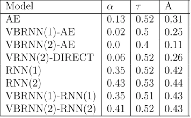
Table 3.5: 𝑅2 for Models of Two-Layer Recovery of Generating Parameters for VDP
Model 𝛼 𝜏 A AE 0.13 0.52 0.31 VBRNN(1)-AE 0.02 0.5 0.25 VBRNN(2)-AE 0.0 0.4 0.11 VRNN(2)-DIRECT 0.06 0.52 0.26 RNN(1) 0.35 0.52 0.42 RNN(2) 0.43 0.53 0.44 VBRNN(1)-RNN(1) 0.35 0.51 0.43 VBRNN(2)-RNN(2) 0.41 0.52 0.43
Table 3.6: 𝑅2 for Models of One-Layer Recovery of Generating Parameters for MG
Model 𝜏 𝜎2 AE 0.15 0.0 VBRNN(1)-AE 0.92 0.0 VBRNN(2)-AE 0.93 0.01 VBRNN(2)-DIRECT 0.87 0.0 RNN(1) 0.95 0.86 RNN(2) 0.98 0.92 VBRNN(1)-RNN(1) 0.97 0.87 VBRNN(2)-RNN(2) 0.98 0.92
Table 3.7: 𝑅2 for Models of Two-Layer Recovery of Generating Parameters for MG Model 𝜏 𝜎2 AE 0.87 -0.15 VBRNN(1)-AE 0.93 0.01 VBRNN(2)-AE 0.94 0.0 VBRNN(2)-DIRECT 0.91 0.01 RNN(1) 0.97 0.82 RNN(2) 0.99 0.89 VBRNN(1)-RNN(1) 0.98 0.87 VBRNN(2)-RNN(2) 0.99 0.93
Table 3.8: VDP Clustered Dataset 1
Model Cluster 1 Min Cluster 1 Max Custer 2 Min Cluster 2 Max
𝛼 4 7 7 11
𝜏 1 15 15 30
A 1 6 6 10
performing in the case of 𝜎2 for the MG dataset. The latter is particularly notewor-thy since the AE, VBRNN-AE and VBRNN-DIRECT models encode no information about the noise at all, while the RNN and VBRNN-RNN models have excellent re-covery of noise 𝜎2 with 𝑅2 values above 0.85. Notably, however, the VBRNN-RNN
models do not give consistently better parameter recovery than the RNN model. This is not altogether unexpected, given that the VBRNN-RNN only extracts information from the RNN and does not obtain any new data not already present. This suggests that the VBRNN models do not improve upon feature recovery over existing tech-niques, but do indicate that VBRNN-RNN models encode significantly more latent parameter information than the VBRNN-AE and VBRNN-DIRECT variants.
3.3.3
Supervised Cluster Recovery in Latent Space
We next present an experiment that seeks to determine how well the latent space distinguishes clusters within the parameter space. This is similar to recovering the latent parameters as in the previous section, though more realistic in a real world
setting. Exact parameters are often impossible to determine, but identifying outcomes based on these parameters, such as whether a manufacturing run succeeds or fails, can be used to differentiate between regions or clusters in the parameter space.
To explore this in a synthetic dataset, VDP datasets are generated with explicit clusters in the parameter space as described in Section 3.1.4. The datasets are gener-ated from the same differential equation with multiple possibly overlapping clusters defined 𝑎1...𝑎𝑁 and mixing parameters 𝑝1...𝑝𝑛. Individual trajectories within each dataset are generated as follows. First, a parameter cluster 𝑎𝑖 is selected with
proba-bility 𝑝𝑖, then parameters are drawn uniformly at random from the parameter cluster, and used to generate a trajectory. Models are trained on this dataset in an unsuper-vised manner, then the respective 𝑉𝑚𝑜𝑑𝑒𝑙 are used to train a classifier 𝑃 (𝑎𝑖|𝑉𝑚𝑜𝑑𝑒𝑙).
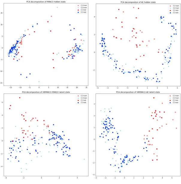
To test relatively ideal conditions, two disjoint clusters are selected as shown in Table 3.8. Cluster 1 is selected with 88% probability and cluster 2 with 12% probability, to model class imbalance often found in clusters in real world datasets. 100 trajectories are generated, with this number selected to mirror possibly small real-world datasets. Training these models and then graphing their latent states as described in Section 3.3.1 and coloring according to the cluster gives the results in Figure 3-6. All but the RNN model show clear separation between the clusters, but the AE performs particularly well in that the clusters are very clearly visible and separated. The RNN model shows very little separation between the clusters, yet the VBRNN model was able to learn a transformation clearly separating the two, when conditioned on either the AE or the RNN.
3.3.4
Anomaly Detection from Latent Space
Anomaly detection is similar to clustering, with the distinction that we only see a subset of clusters in the training set. We wish to identify trajectories that do not come from the same generating distribution as the training set. To do this we train a classifier 𝜑𝑚𝑜𝑑𝑒𝑙 that learns the correlation structure of 𝑉𝑚𝑜𝑑𝑒𝑙 and outputs a probability that a given input is drawn from the same distribution as 𝑉𝑚𝑜𝑑𝑒𝑙. We
and negative datapoints are sampled dimension-wise independent from 𝑉𝑚𝑜𝑑𝑒𝑙. The generated negative datapoints thus follow the same distribution as 𝑉𝑚𝑜𝑑𝑒𝑙 in each of
the dimensions, but are independent and contain no correlation structure. For models with a prior such as the AE and VBRNN, we can simply sample from the prior. We then train 𝜑𝑚𝑜𝑑𝑒𝑙 to classify this dataset. This is akin to performing a hypothesis test with null hypothesis that a given vector is drawn from the same distribution as 𝑉𝑚𝑜𝑑𝑒𝑙, and alternative hypothesis that the given datapoint is drawn from the prior. The alternative hypothesis thus indicates an anomaly.
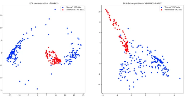
Models of this form are trained on both the MG and VDP datasets. Once trained, a test dataset consisting of half VDP and half MG is used for both, with the other dynamics not used for training considered the anomalous data. Unfortunately, for the purposes of anomaly detection, all of the VBRNN models are significantly out-performed by the autoencoder and RNN models. In fact some of the VBRNN models fail to have any predictive power in this anomaly detection setup. Looking closer, this seems to be due to the fact that the VBRNN models are extracting time-constant features; see Figure 3-7 for an example. Since the RNN contains information about the dynamics of the modelled trajectory, MG trajectories appear very distinguishable from VDP trajectories. For the VBRNN(2)-RNN(2) model, there is significant over-lap since no information about the dynamics are present. This indicates a flaw with this method of anomaly detection, since we are not using a significant portion of the information present in the VBRNN models. While anomaly detection is not further explored in this thesis, Section 4.3 suggests further ideas and techniques that could address this problem.
3.3.5
Evolution of Latent Space from Different Samplings
We next consider the evolution of the latent space, under different trajectory sam-ples. For the VBRNN model, if perfect disentanglement is achieved then for a given stationary trajectory, 𝑉𝑉 𝐵𝑅𝑁 𝑁 should be constant regardless of where the input sub-segment is sampled from. Of course, we do not expect perfect disentanglement given limited data, and thus we wish to explore how 𝑉𝑚𝑜𝑑𝑒𝑙 is affected by where the input