HAL Id: insu-01164245
https://hal-insu.archives-ouvertes.fr/insu-01164245
Submitted on 9 Nov 2015
HAL is a multi-disciplinary open access
archive for the deposit and dissemination of
sci-entific research documents, whether they are
pub-lished or not. The documents may come from
teaching and research institutions in France or
abroad, or from public or private research centers.
L’archive ouverte pluridisciplinaire HAL, est
destinée au dépôt et à la diffusion de documents
scientifiques de niveau recherche, publiés ou non,
émanant des établissements d’enseignement et de
recherche français ou étrangers, des laboratoires
publics ou privés.
www.atmos-chem-phys.net/15/12327/2015/ doi:10.5194/acp-15-12327-2015
© Author(s) 2015. CC Attribution 3.0 License.
Ice water content vertical profiles of high-level clouds: classification
and impact on radiative fluxes
A. G. Feofilov1, C. J. Stubenrauch1, and J. Delanoë2
1Laboratoire de Météorologie Dynamique, IPSL/CNRS, UMR8539, Ecole Polytechnique, France 2LATMOS/UVSQ/IPSL/CNRS, Guyancourt, France
Correspondence to: A. G. Feofilov ([email protected])
Received: 1 April 2015 – Published in Atmos. Chem. Phys. Discuss.: 16 June 2015 Revised: 8 October 2015 – Accepted: 22 October 2015 – Published: 9 November 2015
Abstract. In this article, we discuss the shape of ice wa-ter content (IWC) vertical profiles in high ice clouds and its effect on their radiative properties, both in short- and in long-wave bands (SW and LW). Based on the analysis of collocated satellite data, we propose a minimal set of prim-itive shapes (rectangular, isosceles trapezoid, lower and up-per triangle), which represents the IWC profiles sufficiently well. About 75 % of all high-level ice clouds (P < 440 hPa) have an ice water path (IWP) smaller than 100 g m−2, with a 10 % smaller contribution from single layer clouds. Most IWC profiles (80 %) can be represented by a rectangular or isosceles trapezoid shape. However, with increasing IWP, the number of lower triangle profiles (IWC rises towards cloud base) increases, reaching up to 40 % for IWP values greater than 300 g m−2. The number of upper triangle profiles (IWC rises towards cloud top) is in general small and decreases with IWP, with the maximum occurrence of 15 % in cases of IWP less than 10 g m−2. We propose a statistical classifi-cation of the IWC shapes using IWP as a single parameter. We have estimated the radiative effects of clouds with the same IWP and with different IWC profile shapes for five typ-ical atmospheric scenarios and over a broad range of IWP, cloud height, cloud vertical extent, and effective ice crystal diameter (De). We explain changes in outgoing LW fluxes at the top of the atmosphere (TOA) by the cloud thermal radiance while differences in TOA SW fluxes relate to the De vertical profile within the cloud. Absolute differences in net TOA and surface fluxes associated with these parameter-ized IWC profiles instead of assuming constant IWC profiles are in general of the order of 1–2 W m−2: they are negligible for clouds with IWP < 30 g m−2, but may reach 2 W m−2for clouds with IWP > 300 W m−2.
1 Introduction
Clouds play an important role in the energy budget of our planet: optically thick clouds reflect the incoming solar radi-ation, leading to cooling of the Earth, while thinner clouds act as “greenhouse films”, preventing escape of the Earth’s long-wave (LW, see also Table A1 in the Appendix; this is not explained in the text for readability’s sake) radiation to space. Understanding the Earth’s radiative energy budget re-quires knowing the cloud cover, thermodynamic phase (ice, liquid, mixed phase), height, temperature, and thickness, as well as the optical properties of cloud particles and their con-centration. In this article, we address the shape of the ice wa-ter content profile, IWC(z), for high ice clouds (defined by pressure less than 440 hPa and including only ice particles).
Satellite observations provide a continuous survey of clouds over the whole globe. IR (infrared) sounders have been observing our planet since 1979: from the TOVS (Tele-vision Infrared Observation Satellite) sounders (Smith et al., 1979) onboard the NOAA polar satellites to the AIRS (At-mospheric Infrared Radiation Spectrometer) (Chahine et al., 2006) onboard Aqua (since 2002) and to the IASI (Infrared Atmospheric Sounding Interferometer) (Chalon et al., 2001; Hilton et al., 2012) onboard MetOp (since 2006), with in-creasing spectral resolution. Their spectral resolution along the CO2absorption band makes IR (infrared) sounders
sen-sitive to cirrus, day and night (Stubenrauch et al., 1999, 2006, 2008, 2010; Wylie et al., 2005). In addition, they provide atmospheric temperature and water vapour profiles, surface temperature, and dust aerosol properties. Vertical profiles of the cloud parameters are available from active sensors: since 2006, the CALIPSO (Cloud Aerosol Lidar and Infrared
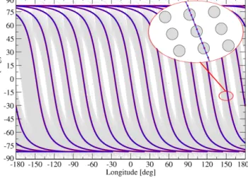
Figure 1. Latitude/longitude coverage for 1 July 2008, observation time 13:30 (at the equator crossing time). Grey: AIRS footprints; red: CALIPSO L2 cloud data at 5 km resolution; blue: CloudSat footprints. The centre of a blown-up part of the orbit corresponds to (lat = −25◦; lon = 154◦).
Pathfinder Satellite Observation) (Winker et al., 2003) and CloudSat radar (Stephens et al., 2002), together, observe the atmosphere. Whereas the lidar is highly sensitive and can even detect sub-visible cirrus, its beam reaches cloud base only for clouds with an optical depth less than 3. When the optical depth is larger, the radar is still capable of pene-trating the cloud down to its base. The DARDAR products (raDAR/liDAR, Delanoë and Hogan, 2010), retrieved from these radar and lidar measurements, provide vertical profiles of thermodynamic cloud phase, IWC(z) and De(z) with a fine vertical resolution, essential for our analysis.
The structure of the article is as follows. In Sect. 2, we de-scribe the data sets used in this study and the colocation ap-proach. Section 3 presents the statistical results of the collo-cated data and describes the classification into different types of ice cloud profiles and their occurrence in dependence of different atmospheric parameters. In Sect. 4, we estimate the radiative effects on the IWC(z) profile shape. Section 5 sum-marizes the results.
2 Data sets
The analysis builds on the synergy of the NASA Afternoon Constellation (A-Train) mission (Stephens et al., 2002), pro-viding observations at 01:30 and 13:30 local time (LT), at the equator crossing. Table 1 lists the Level 2 data sets and the specific variables used in this analysis. The following sub-sections provide brief information on the corresponding in-strument, and retrieval methodology.
rauch et al., 2010). Briefly, the retrieval methodology is based on a weighted χ2method using radiances measured along the wing of the 15 µm CO2absorption band. The χ2method
de-termines the cloud pressure level (pcld), for which the
mea-sured radiances provide the most coherent cloud emissiv-ity. The method also yields IR cloud emissivity defined as
εcld=(Iclear−Imeas)/(Iclear−Icld(pcld)), where Imeasis the
measured radiance, Iclearis the clear sky radiance and Icldthe
radiance of an optically thick cloud at the pcldlevel estimated
for the observed situation from a minimum in the χ2vertical profile. The AIRS-LMD data set participated in the GEWEX cloud assessment (Stubenrauch et al., 2013) and performed well. In the case of multiple cloud layers, the retrieved prop-erties correspond to those of the highest cloud layer, as far as its optical depth is above 0.1.
2.2 CALIPSO cloud data at 5 km spatial resolution
CALIOP (Cloud-Aerosol Lidar with Orthoganal Polariza-tion), a two-wavelength polarization-sensitive nadir viewing lidar, provides high-resolution vertical profiles of aerosols and clouds. It uses three receiver channels: one measuring the 1064 nm backscatter intensity and two channels measuring orthogonally polarized components of the 532 nm backscat-tered signal. Cloud and aerosol layers are detected by com-paring the measured 532 nm signal return with the return ex-pected from a molecular atmosphere. The method utilizes an adaptive threshold test (Vaughan et al., 2009) and retrieved the height of the physical top height, rather than the effec-tive radiaeffec-tive height. The method is capable of detecting the clouds with visible extinction as small as ∼ 0.01 km−1 though the detection efficiency decreases in this domain and, as Davis et al. (2010) have shown, the CALIPSO misses a certain fraction of sub-visible cirrus clouds. The retrieval al-gorithm is the same for the daytime and nighttime portions of the orbit, except that different detection thresholds are used for day and night. Analysis of the parallel and perpendicular polarization of 532 nm backscatter signals provides vertically resolved identification of cloud water phase according to the algorithm of Hu et al. (2007). For this analysis, we utilize
ztopand zbasefrom version 3 of the CALIPSO L2 cloud data
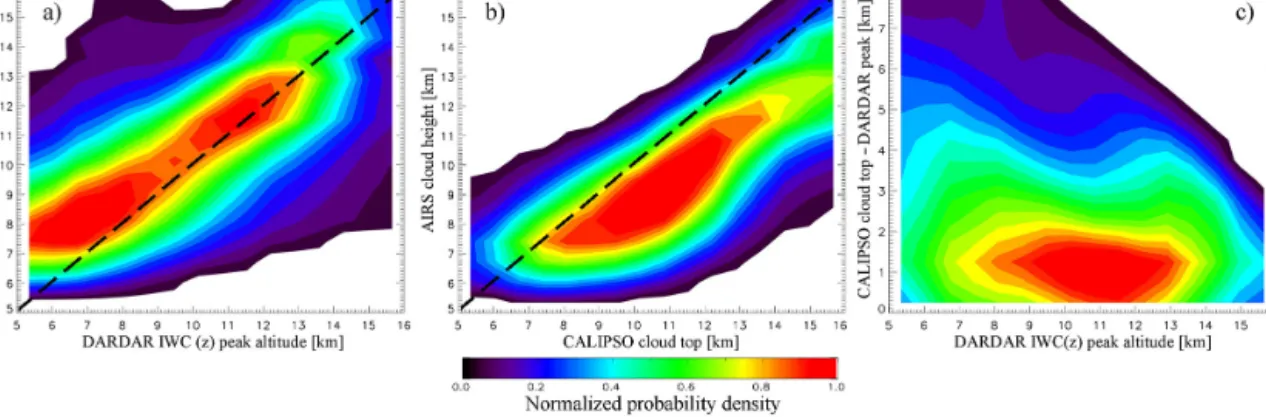
Table 1. L2 data sets and products used in this analysis. L2 Data set Variables
AIRS-LMD Cloud pressure (pcld), cloud temperature (Tcld), cloud emissivity (εcld), cloud height (zcld)
CALIPSO 5km clouds cloud top height (ztop), effective cloud base height (zbase)for multiple cloud layers
Radar-lidar GEOPROF ztopand zbasefor multiple cloud layers
DARDAR IWC(z), De(z), cloud type vertical profiles ERA-Interim vertical wind
2.3 CloudSat geometrical profiling product (GEOPROF)
The GEOPROF L2 product (Haynes and Stephens, 2007; Haladay and Stephens, 2009; Mace et al., 2009) of version P1_R04 merges the millimetre wavelength cloud profiling radar (CPR) radar data (footprint of 2.5 km × 1.4 km) with those collected by CALIOP. CloudSat shares an orbit with CALIPSO, so that they probe nearly the same volumes of the atmosphere within 10–15 s of each other. This configuration combined with the capacity for millimetre radar to penetrate optically thick hydrometeor layers and the ability of the lidar to detect optically thin clouds has allowed Mace et al. (2009) to develop an approach for retrieving the vertical and hor-izontal structure of hydrometeor layers with unprecedented precision, ranging from optically thin cirrus and boundary layer clouds to deep optically thick precipitating systems. In this study, the GEOPROF product helps us to verify if the cloud base height for the selected overlap is consistent with the IWC profile provided in the DARDAR data set (see next section) and use the ztopvalues to “align” the IWC(z) profiles
for the classification (Sect. 3.2).
2.4 Lidar-Radar synergy of the DARDAR data set
Delanoë and Hogan (2010) have adapted a variational method using the synergy of radar, lidar, and infrared ra-diometer from airborne and ground-based measurements (Delanoë and Hogan, 2008) to CALIPSO-CloudSat-MODIS satellite observations to retrieve vertical profiles of visible extinction coefficient, IWC, and De. The variational scheme finds a state vector x, which minimizes the square-root sum of the differences between the observed (y) and calcu-lated radiances. The components of the observation vector
y are the following: radar reflectivity factor, apparent lidar
backscatter as well as IR radiance and IR radiance difference if the radiometer is used. Note that in the version we are us-ing the IR radiances are not assimilated. The components of
x are the visible extinction coefficients at different altitudes,
extinction-to-backscatter ratio, and number concentration pa-rameters at different altitudes.
The solution (state vector x) is found by minimizing a cost function using Gauss–Newton iteration, as described fully by Delanoë and Hogan (2008). A key input to the retrieval algo-rithm is an observational error covariance matrix, which
in-cludes both instrument and forward-model errors (Delanoë and Hogan, 2008, 2010). The resulting DARDAR (for li-DAR + rali-DAR) products contain the profiles of the ice cloud related parameters on a 60 m vertical grid, which have been used in a number of studies (Bardeen et al., 2013; Battaglia and Delanoë, 2013; Ceccaldi et al., 2013; Delanoë et al., 2011, 2013; Deng et al., 2013; Eliasson et al., 2012; Faijan et al., 2012; Gayet et al., 2014; Huang et al., 2012; Jouan et al., 2012, 2014; Mason et al., 2014; Stein et al., 2011a, b).
2.5 ERA-Interim
ERA-Interim global atmospheric reanalysis is produced by the European Centre for Medium-Range Weather Forecasts (ECMWF), covering the period from 1989 until now. Dee et al. (2011) give a detailed description of the approach and the data. The data assimilation scheme is sequential: at each time step, it assimilates available observations to constrain the model built with forecast information obtained in the pre-vious step. The analyses are then used to make a short-range model forecast for the next assimilation time step. Gridded data products (at a spatial resolution of 0.75◦latitude × 0.75◦ longitude) also include 6-hourly dynamic parameters such as horizontal and vertical large-scale winds. A common proxy for the intensity of the vertical motions in the atmosphere is the vertical pressure velocity at 500 hPa level, w500 (e.g.
Bony and Dufresne, 2005; Martins et al., 2011). In addition, we also use vertical winds just underneath the cloud (wbase)
and at the radiative height of the cloud (wcloud)to study
cor-relations between the shape of the cloud IWC profile and the atmospheric dynamics.
2.6 Colocation of the data sets
Figure 1 illustrates a typical single-day coverage of AIRS and CALIPSO-CloudSat at a specific observation time (13:30 at the equator crossing time). Whereas the AIRS swaths cover areas about 1000 km, the active instruments only cover a 90 m–1.4 km wide track near the middle of the AIRS swaths. Since the instruments share the same orbit, one can impose strict overlapping criteria to get a high-quality data set.
Our colocation starts with the AIRS data and searches the other data sets for the observations closest to the centres of individual AIRS footprints (usually, three per each golf ball). A blown-up part in the upper-right corner of Fig. 1
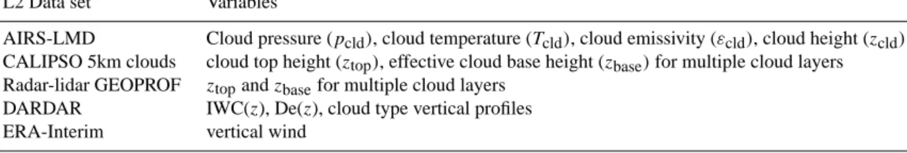
Figure 2. Examples of the IWC profiles of high ice clouds, including information on cloud height from the collocated AIRS-LMD, CALIPSO, GEOPROF, and DARDAR data, for clouds with increasing IWP values. Black curves: DARDAR IWC(z) profile; coloured horizontal lines mark the position of the AIRS cloud, CALIPSO and GEOPROF cloud top and cloud base heights. All profiles are for July 2007: (a) lat = 2.3◦, lon = −15.9◦; (b) lat = 23.9◦, lon = 101.7◦; (c) lat = 0.3◦, lon = 101.8◦; (d) lat = −2.5◦, lon = 120.6◦.
Table 2. Colocation statistics corresponding to the data illustrated in Fig. 1.
Data set Nday % selected rms dist
with respect to orig. [km]
AIRS-LMD 1.5 × 10⁶ 0.4 0 (self)
CALIPSO 1.1 × 10⁵ 9.4 6.1
GEOPROF 5.5 × 10⁵ 2.0 5.78
DARDAR 5.5 × 10⁵ 2.0 5.78
ERA-Interim 4.6 × 10⁵ 3.6 24.0
shows an example of the overlapping measurements: for favourable conditions, the AIRS footprint can cover up to three CALIPSO L2 samples at 5 km resolution and up to 10 GEOPROF/DARDAR L2 samples at the spatial resolution of a CPR footprint (1.7 × 1.4 km). One has to keep in mind that “ideal” overlaps like the one shown in Fig. 1 are not so frequent: if the closest CALIPSO or DARDAR footprint lies outside the AIRS footprint, then the case is skipped.
Table 2 complements Fig. 1 and shows the statistics for the components of the collocated data set. As one can see, with the rigid colocation criteria used in this work the av-erage distance between the centres of the samples is about 6 km. The fraction of the data selected is small, but the num-ber of overlaps per day is still on the order of ∼ 1 × 10⁴. The temporal deviation between the observations is defined by the distance between the satellites and is less than 2 min. The ERA-Interim atmospheric reanalysis deviates on aver-age much more because of its rather coarse spatial and time resolution. The resulting collocated data set comprises the variables listed in Table 1.
3 Analysis
3.1 Selecting high-level ice clouds
Figure 2 illustrates the information available in the collocated data set, for typical examples of high-level ice clouds, with IWP (ice water path) increasing from 9.0 to 303 g m−2. In this figure, we supplement the IWC vertical profiles with AIRS zcld (horizontal red lines), CALIPSO ztop and zbase
(blue lines), and GEOPROF ztopand zbase(green lines). It is
interesting to trace the behaviour of these values with chang-ing IWP: whereas CALIPSO and GEOPROF ztopmatch on
all four panels, CALIPSO and GEOPROF zbase match at
IWP < 100 g m−2, while the CALIPSO lidar cannot probe the lower boundary of thicker clouds; AIRS zcldcorresponds
to the radiative height close to the maximum backscatter sig-nal from CALIPSO (Stubenrauch et al., 2010); for high-level ice clouds it lies generally 1 to 2 km below cloud top, de-pending on the vertical accumulation of optical depth (Liao et al., 1995; Holz et al., 2008); it seems to correspond to the IWC peak height up to IWP of about 30 g m−2, while for thicker clouds the corresponding optical depth is reached earlier. We explain all these features by the capabilities of the instruments and by physics of observations, and we find them to be consistent with the results presented elsewhere (e.g. Stubenrauch et al., 2013, and references therein). For the analysis, we have selected only high ice clouds, using AIRS cloud pressure (pcld<440 hPa) and DARDAR profile
information on the occurrence of liquid or ice. To ensure high quality of the selected subset, we filtered out the cases, for which DARDAR ice cloud peak height is beyond the GEO-PROF ztopand zbaselimits of the layer, closest to the AIRS
cloud. This removes 18 % of the collocated data, and the mis-matches are explained by different spatial resolution of the compared data sets, by the uncertainties of pcld→zcld
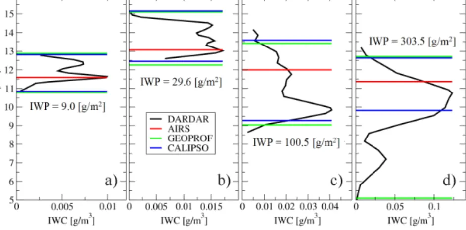
con-Figure 3. Probability density plots of height comparisons for high ice clouds for the whole globe in January 2007: (a) AIRS zcldvs. DARDAR
peak height; (b) AIRS zcldvs. CALIPSO ztop; (c) CALIPSO ztop– DARDAR peak vs. DARDAR. Dashed lines in (a) and (b): one-to-one
correlation.
version associated with temperature/H2O profiles, and by the
GEOPROF cloud boundary thresholds.
Figure 3 shows the comparison of height for all high ice clouds in the collocated and filtered data set. In Fig. 3a, we compare the AIRS cloud height with the DARDAR IWC(z) peak height. As one can see, for clouds above ∼ 10 km the highest probability density (in red) almost follows a 1 : 1 line, while for the lower clouds AIRS tends to be ∼ 2–3 km higher. This is linked to the optical thickness of the cloud and its correlation with the vertical extent: for geometrically thicker clouds, AIRS retrieves the radiative height, while active in-struments are capable of penetrating deeper. In Fig. 3b, AIRS cloud height is compared with the CALIPSO top: 80 % of the clouds are below the CALIPSO cloud top boundary; we as-sign the remaining 20 % to difference in sample size of these two instruments (5 km × 0.06 km vs. 15 km × 15 km) and to accuracy in AIRS cloud height determination (1 km). The purpose of Fig. 3c is to show the spread of the IWC(z) pro-file within the cloud: for the clouds peaking in the 8–13 km region, their ztopis usually just 1 km higher than the peak;
however, the distribution is broad and for a significant frac-tion of clouds with smaller emissivity the IWC(z) maximum is much lower than the ztop. This is consistent with the AIRS
vs. DARDAR peak plot in Fig. 3a: the IWC peak of extended cloud layers is closer to cloud base.
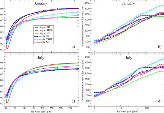
Figure 4 presents average cloud emissivity and verti-cal extent in relation to IWP. As one can see, average IR cloud emissivity increases with IWP and then saturates at
∼0.7–0.9 for IWP values greater than ∼ 100 g m−2.
How-ever, for the same large IWP, the mean is smaller in win-ter midlatitudes than in summer midlatitudes. It is inwin-terest- interest-ing to note the peculiarity of ε(IWP) curves in the low IWP domain (Fig. 4a, c), where ε increases for IWP values less than ∼ 4–7 g m−2. One has to keep in mind that the same amount of water can form clouds of different optical depths (and emissivities): for thin clouds, the ice crystal size dis-tribution centres around lower values compared to that of
thicker clouds. We justify this explanation by building the
ε(IWP) distributions only for De > 40 µm (not shown for the sake of clarity). These distributions do not have a feature at IWP ≈ 4–7 g m−2; instead, the ε(IWP) increases mono-tonically and then reaches saturation. The relationship be-tween the vertical extent of the ice cloud (1zcld) and its
IWP is shown in Fig. 4b, d. Here one has to note the dif-ference between the summer and winter hemispheres: both single and multi-layer clouds show a saturation of 1zcldin
the winter hemisphere at IWP ≈ 70 g m−2 that corresponds to higher ice water densities in the storm tracks. Another re-markable feature of the 1zcld(IWP) is a nearly linear
depen-dence on log(IWP) (with the exception for aforementioned saturation effects in winter hemispheres). This allows reduc-ing the number of variables in the statistical classification we seek to develop.
Table 3 shows the latitudinal behaviour of cloud emis-sivity, IWP, vertical extent and proportion of ice within the cloud, separately for single-layer and multi-layer cloud scenes (identified by GEOPROF). We draw the readers’ at-tention to two types of IWP values in Table 3: median and mean IWPs. The median IWPs are calculated over the ensemble of corresponding cloudy scenes, while the mean IWPs represent both cloudy and clear sky scenes together. The latter distribution shows a common three-peak pattern (cf. Eliasson et al., 2011) while the median values are more representative for strongly skewed distributions, which is the case of the IWP. As one can see, single layer high clouds are thicker both in geometrical and in optical sense. One can note the following differences: (a) median IWP values differ more strongly than cloud emissivities that is related to cloud emissivity saturation for thick clouds; (b) the vertical extent
1zcld of single layer clouds is ∼ 0.7 km larger than that of
top ice clouds in multi-cloud scenes; (c) the geometrical ra-tio of ice layer thickness with respect to total layer thickness (1zice/1zcld)is larger for single layer clouds. We associate
Figure 4. Average cloud emissivity and ice cloud layer vertical extent as a function of ice water path, separately for single and multi-layer clouds and three latitude zones, for 2 months (January 2007: a, b, and July 2007: c, d). All four panels share the same legend, SH (Southern Hemisphere), TROP (tropical type atmosphere), and NH (Northern Hemisphere) correspond to latitude zones 90–30◦S, 30◦S–30◦N, and 30–90◦N, respectively.
which the conditions at the lower boundary of high ice cloud are favourable for changing the phase from ice to water.
3.2 Approximating the ice water content profiles with primitive shapes
We have analyzed the IWC profiles with respect to cloud IWP, vertical extent, latitude, and atmospheric dynamics. The objectives of this analysis are the following: (a) establishing a minimal basis of primitive shapes, which one can use for approximating IWC(z), (b) building a statistical model for these primitive profiles, and (c) estimating the energetic ef-fects of clouds with the same ice water path (IWP) but dif-ferent IWC(z). A “minimal basis” in this context means that the individual elements of the suggested set of IWC profiles should not be linearly dependent with respect to any of the at-mospheric and cloud variables. We have “aligned” the IWC profiles using the GEOPROF ztopvalues, calculated the
ver-tical extent of the ice cloud using the GEOPROF zbase and
ztopvalues, determined the IWP by integrating the DARDAR
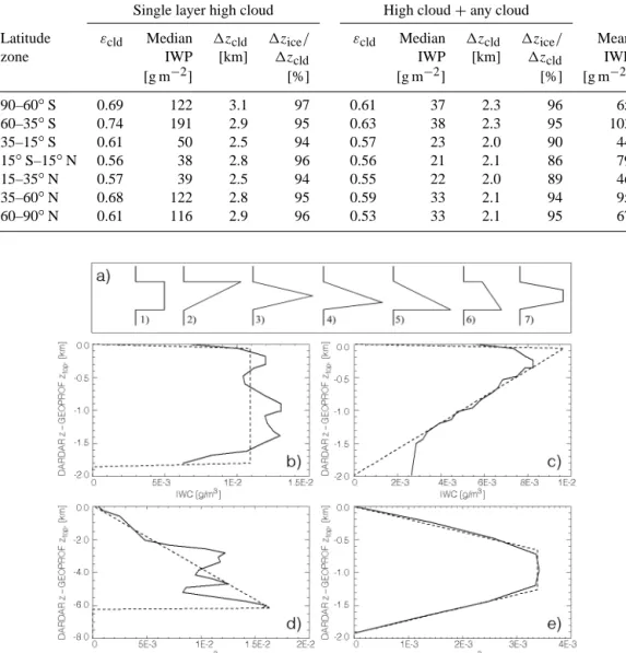
IWC(z) within these limits, normalized the IWC profiles to IWP, and compared them with a set of primitive shapes. An initial set of shapes consisted of the following: (1) “rectangu-lar” or constant IWC; (2) “upper triangle”; (3) “isosceles tri-angle”; (4) “tilted tritri-angle”; (5) “lower tritri-angle”; (6) “trape-zoid”; and (7) “isosceles trapezoid”, illustrated in Fig. 5a. The “tilted triangle” was built using the average top-to-peak and base-to-peak IWC(z) gradients normalized by the IWP.
The other shapes are empirical approximations. It is impor-tant to note here that using a fixed set of profile shapes does not mean using the same IWC gradient within the same type: the real IWC values are always bound to the IWP of the cloud through normalizing.
To check the redundancy within these seven primitive pro-file shape types, we have used the statistics built over the globe for 1 month, January 2007 (the results do not change significantly for any other period). For each collocated event and for each primitive shape, we have calculated ζ , a stan-dard rms of the model IWC profile deviation from the real IWC(z) profile. As a result, we have obtained seven se-quences of ζ values and performed a “round robin” corre-lation analysis of these sequences. As the linear correcorre-lation coefficients in Table 4 show, a set of seven profile shapes ap-pears to be redundant since some pairs of profile shapes are strongly correlated, with the correlation coefficients of about 0.8–0.9 (marked in bold), so it is logical to reduce the ba-sis. The first profile to keep is a standard one (rectangular), which is approximated by a constant-within-layer IWC and which corresponds to an assumption currently used in the re-trieval of cirrus bulk microphysical properties (e.g. Guignard et al., 2012). The profiles #2 (upper triangles) and #5 (lower triangles) are uncoupled from the others, so they should also be included to a reduced basis. In addition, we keep shape #7, which fills a gap between #2 and #5 and which is more physically sound compared to #1 (sharp changes in
concen-Table 3. Latitudinal averages of different ice cloud variables.
Single layer high cloud High cloud + any cloud
Latitude εcld Median 1zcld 1zice/ εcld Median 1zcld 1zice/ Mean
zone IWP [km] 1zcld IWP [km] 1zcld IWP
[g m−2] [%] [g m−2] [%] [g m−2] 90–60◦S 0.69 122 3.1 97 0.61 37 2.3 96 65 60–35◦S 0.74 191 2.9 95 0.63 38 2.3 95 103 35–15◦S 0.61 50 2.5 94 0.57 23 2.0 90 44 15◦S–15◦N 0.56 38 2.8 96 0.56 21 2.1 86 79 15–35◦N 0.57 39 2.5 94 0.55 22 2.0 89 46 35–60◦N 0.68 122 2.8 95 0.59 33 2.1 94 95 60–90◦N 0.61 116 2.9 96 0.53 33 2.1 95 67
Figure 5. Cloud IWC(z) examples and their approximation with primitive shapes: (a) initial set of seven profiles; (b) constant-within-layer or rectangular; (c) upper triangle; (d) lower triangle; (e) isosceles trapezoid. Solid lines: DARDAR IWC(z) profile, dashed lines: best fit profile. Height is shown with respect to GEOPROF ztop.
tration are unlikely in high ice clouds, especially in the trop-ics, (e.g. Liao et al., 1995). The reduced set of profiles #1, #2, #5, and #7, illustrated by representative examples of the data and their approximations in Fig. 5, does not contain linearly dependent elements.
3.3 Ice crystal size profile
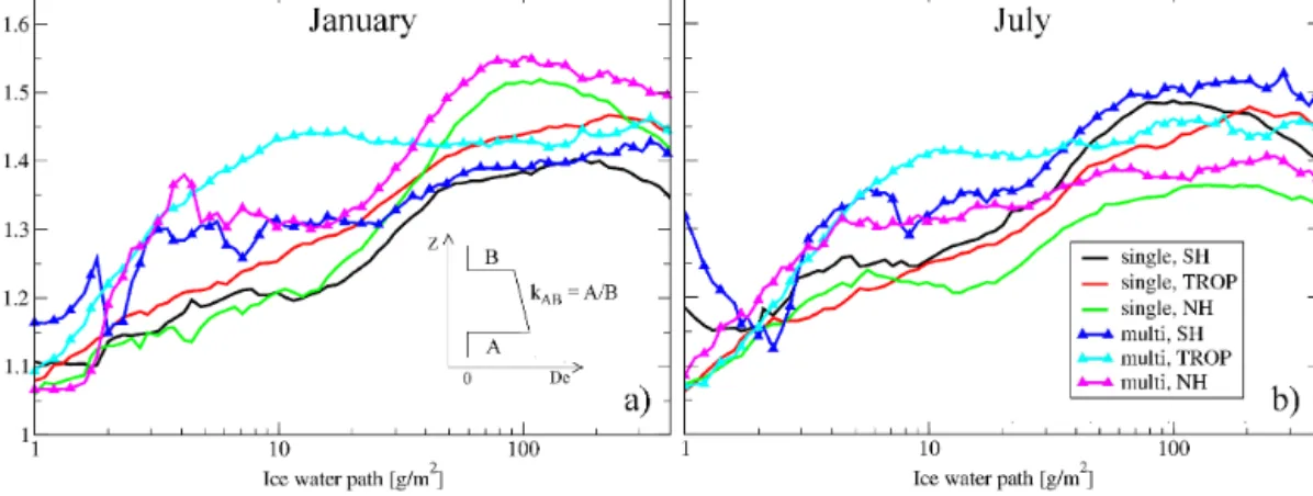
Besides IWC, another important radiative characteristic of the cloud is the effective ice crystal size and its changes with height. The analysis of DARDAR De(z) profiles shows that they are not as diverse as the IWC profiles and can be repre-sented with a trapezoid similar to profile #6 in Fig. 5a. Here, the only parameter needed to describe the vertical profile is the ratio of the upper and lower edges of the trapezoid (kAB,
see a sketch in Fig. 6a). We have studied the best fit of this parameter for different IWPs and seasons, varying kABin a
broad range from 0.1 (almost the “upper triangle”) through 1.0 (rectangular) to 10 (almost “lower triangle”). As one can see in Fig. 6, for IWP < 2 g m−2 De(z) is almost constant (kAB≈1.1) and this coefficient demonstrates only a
mod-erate increase up to IWP ≈ 10 g m−2. This is explained by the low density of the ice particles, which hinders the ag-gregation and buoyancy stratification. For IWP > 30 g m−2, De(z) is best represented by a trapezoid with a ratio of edges
kAB=1.35–1.5. For these densities, the probability of ice
particle aggregation is higher and the sedimentation of heav-ier particles increases their concentration towards the cloud base. It is interesting to compare the behaviour of kAB for
Figure 6. Values of kAB(ratio of the lower and upper edges of the trapezoid fitting De(z) vertical profile) for single and multi-layer cloud
scenes for three latitudinal zones for (a) January and (b) July. The legend is the same as in Fig. 4.
Table 4. Linear correlation coefficients for a monthly series (30 000 samples, January 2007) of ζ deviation values for seven test cloud profiles. Profile # 1 2 3 4 5 6 7 1 1.00 0.62 0.40 0.35 0.43 0.88 0.44 2 – 1.00 0.46 0.08 −0.31 0.22 0.43 3 – – 1.00 0.82 −0.26 0.15 0.99 4 – – – 1.00 0.08 0.31 0.85 5 – – – – 1.00 0.79 −0.22 6 – – – – – 1.00 0.21 7 – – – – – – 1.00
winter and summer midlatitudes as we did for 1zcld(IWP)
distributions in Fig. 4: in winter, kABis larger than in
sum-mer, meaning stronger vertical De(z) gradients during this period. This behaviour is consistent with denser clouds in the storm tracks discussed above. However, De also depends on the mechanism of cirrus formation (e.g. in situ or as an anvil of a convective system), on the life stage of the system and on the environmental temperature and humidity. In this article, we do not study the De profiles in further detail, but, as the estimates in the next section show, the vertical profile of De affects the radiative properties of the cloud and should be taken into account in the analysis and modelling.
4 Results
4.1 Relating IWC profile shapes to cloud and atmospheric parameters
We have analyzed 3 years (2007–2009) of collocated data by searching for the best fit within the four primitive IWC(z) shapes: rectangular, isosceles trapezoid, lower triangle, and upper triangle. Then we have studied their relative occur-rence with respect to IWP, cloud layering (single or multi), cloud vertical extent, vertical wind, latitude and underlying
surface (land or ocean). As a first step, we have studied the probability of occurrence of these specific IWC profile shapes as a function of IWP. Table 5 presents the statistics separately for single-layer and multi-layer cloud scenes, re-spectively. As the median values of Table 3 have already indi-cated, about 75 % of all high ice clouds lie within the range of IWP < 100 g m−2. Within this IWP range, about 60 to 80 % of the IWC profiles may be represented by rectangular (con-stant IWC) and isosceles trapezoid shapes.
As one can see from the normalized IWP histogram val-ues presented in Table 5a and b, the relative frequency of thick ice cloud occurrence is higher in a single- rather than in a multi-layer system. Qualitatively, the IWC profile shape type fractioning behaves the same way for single- and multi-layer cloud scenes: if joined, rectangular and trapezoid IWC shapes make up more than 70 % of all the shapes. Between these two types, trapezoid-like IWC shapes dominate both single- and multi-layer scenes, unless IWP < 10 g m−2. The remaining 20–40 % split into profiles with increasing (lower triangle) and decreasing (upper triangle) IWC towards cloud base. We observe, as expected, an increasing occurrence probability of lower triangle with increasing IWP. Upper tri-angle shapes mostly occur in clouds with IWP < 30 g m−2. This is consistent with the currently accepted ice cloud for-mation model: if the amount of ice in the cloud is low, the particles may form an “inverse” IWC profile, stimulated by updraft or by a favourable combination of water vapour and temperature profiles. If the cloud is thicker, the sedimenta-tion of larger particles leads to a decrease of occurrence of this shape.
To address the influence of large-scale vertical winds, we have analyzed the IWC profile shape statistics with respect to vertical wind w500, wbase(at GEOPROF zbase), and wcloud(at
the AIRS zcld)and split it to three dynamic situations: strong
updraft (w < −175 hPa day−1, 6 % of all the cases), “calm atmosphere” (−175 hPa day−1< w <175 hPa day−1, 93 %), and strong downdraft (w > 175 hPa day−1, 1 %), like those
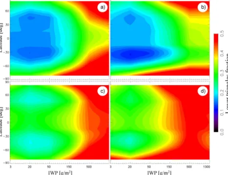
Figure 7. Lower triangles fraction with respect to ice water path and latitude: (a) single layer, ocean; (b) single layer, land; (c) multi-layer scenes, ocean; (d) multi-layer scenes, land. The relative occurrence of IWP bins can be found in Table 5.
used in Stubenrauch et al. (2004). The analysis shows that changes in relative occurrence of IWC profile shapes are only noticeable for strong downdraft within the cloud (see values in brackets in Table 5), while filtering the statistics based on
w500and wbasedid not lead to conclusive results. As one can
see in Table 5, dynamic effects are only well traceable with lower triangles: strong downdrafts correspond to additional 3–11 % occurrence, and the added occurrence grows with IWP. We assign these effects to the following mechanisms: (a) in the case of a downdraft, the whole cloud becomes sub-saturated and the small ice crystals at the top sublimate much faster than the large ones (the size of crystals in the ice cloud increases from top to bottom, see Fig. 6), giving rise to lower triangle profiles; (b) downdraft leads to more intensive aggre-gation of ice crystals within an existing layer of less buoyant ice crystals beneath – this works only when the ice crystal aggregation is noticeable (warm cirrus and completely frozen mixed phase clouds; Kienast-Sjogren et al., 2013). It is inter-esting to note that the situation does not inverse in the case of strong updrafts and the occurrence of upper triangle profiles does not increase. When a strong updraft takes place, a ho-mogeneous freezing is triggered and a lot of small ice crystals appear within the whole cloud (Kärcher and Lohmann, 2002) that leads to an increase in the occurrence of rectangular-type profiles.
In a further step, we address the effects of other factors, which might be important for the statistical IWC profile clas-sification. These are cloud vertical extent 1zcld, latitude
(sea-son), and underlying surface type (land or ocean). The ulti-mate goal is to reduce the number of variables to a necessary
minimum. We already know from Fig. 4b, d that cloud ver-tical extent is almost linearly dependent on the logarithm of IWP, so we only keep IWP for the classification. As for the latitude, Fig. 7 presents the fraction of lower triangles as a function of latitude and IWP. This profile shape is the third one in frequency of occurrence (Table 5) and its radiative ef-fects are expected to differ from those of the first two types (see Sect. 4.2 for the discussion). In Fig. 7, we separate the statistics for single-layer and multi-layer cloud scenes and for ocean and land. As the comparison of Fig. 7a, c with Fig. 7b, d shows, the surface does not have a significant influ-ence on the relative occurrinflu-ence, thus allowing to merge the statistics for land and ocean. On the other hand, single- and multi-layer scenes in Fig. 7a, b and Fig. 7c, d show different patterns, justifying considering them separately. Latitudinal variability for single-layer scenes (Fig. 7a, b) is noticeable in the high IWP domain (> 300 g m−2), but as Table 5 shows,
these cases represent less than 20 % of single layer clouds and less than 10 % of all clouds.
Summarizing, we suggest using the statistical classifica-tion of the IWC profile shape based solely on IWP. We ex-plain relative consistency of the IWC profile shape type frac-tioning by a similarity of cloud formation processes in the atmosphere: regardless of the pressure/temperature/humidity profile, geographic location, and season, the physics of ice nucleation remains the same: once the supersaturation con-ditions and (in the case of a heterogeneous freezing) the ice nuclei exist, the clouds start forming; once formed, ice crys-tals start growing and sedimenting; reaching the zone with
IWP Rectangular Isosceles Lower Upper Relative [g m−2] trapezoid triangle triangle occurrence
0–10 39 31 11 19 22 10–30 29 47 14 10 29 30–100 27 51 16 (+3) 6 27 100–300 21 56 20 (+10) 3 13 300–1000 19 52 27 (+9) 2 6 >1000 19 41 40 1 2
kinetic temperature greater than frost point temperature leads to ice sublimation.
4.2 The impact of IWC profile shape on cloud radiative effects
As mentioned above, ice clouds affect radiative energy bal-ance in the atmosphere in several ways: reflecting and scat-tering the incoming solar radiation, reflecting and scatter-ing terrestrial and atmospheric radiation comscatter-ing from be-low, and emitting infrared radiation in all directions. For a fixed IWP, each of the aforementioned components can de-pend on the profile of absorbing/scattering/emitting particle concentration. In this section, we address radiative effects in the long-wave (LW, 10–3280 cm−1)and short-wave (SW, 820–50 000 cm−1)bands. To quantify them, we will use sur-face radiative flux (SRF), top of the atmosphere radiative flux (TOA), and atmospheric contribution (ATM = TOA − SRF). In a numerical experiment described below, we estimate the effects of the shape of IWC profiles using five typical at-mospheric scenarios: subarctic and midlatitude summer and winter as well as the tropics. The atmospheres were consid-ered up to the mesopause region. The detailed description of atmospheric scenarios and vertical profiles of temperature and atmospheric constituents can be found in Feofilov and Kutepov (2012).
4.2.1 Radiative transfer model RRTM
The calculations have been performed with the help of RRTM (Rapid Radiative Transfer Model) which utilizes the correlated-k approach to calculate fluxes. The software
pack-age consists of RRTM LW (Mlawer et al., 1997; Iacono et al., 2000; Morcrette, 2001) and RRTM SW (Mlawer and Clough, 1997, 1998) modules, both of which use k distributions obtained from an exact line-by-line radiative transfer code (LBLRTM) (Clough et al., 2005). The RRTM LW algorithm calculates the fluxes and cooling rates over 16 LW bands with accuracy at all levels better than 1.5 W m−2and 0.3 K day−1, correspondingly. The optical properties of ice clouds are cal-culated for each spectral band using the Streamer model v3.0 (Key and Schweiger, 1998). The RRTM SW algorithm cal-culates the fluxes over 14 SW bands with accuracy at all lev-els better than 1.0 W m−2for direct and 2.0 W m−2for dif-fuse irradiances (Oreopoulos et al., 2012). Scattering calcu-lations are performed using the DISORT (Discrete Ordinates Radiative Transfer Program) package (Stamnes et al., 1988). For each spectral band, the optical properties of water and ice clouds are calculated using the Hu and Stamnes (1993) and Fu (1996) parameterizations, respectively. With the help of the RRTM code, we have performed a series of radia-tive transfer calculations, varying the atmospheric scenario, De(z) (10 values), IWC(z) profile shape, IWP (seven inter-vals), cloud vertical extent (1zcld, seven values), and cloud
top height (five values). In addition, we doubled the number of simulations by adding an underlying optically thick water cloud to estimate the IWC profile effects when the terrestrial radiance is “blocked”. Overall, the number of simulations is equal to 5 × 10 × 4 × 7 × 7 × 5 × 2 = 98 000. Since the spread of tropical IWP values is larger than that at other latitudes (e.g. Eliasson et al., 2011), we present comparisons for the tropical scenario.
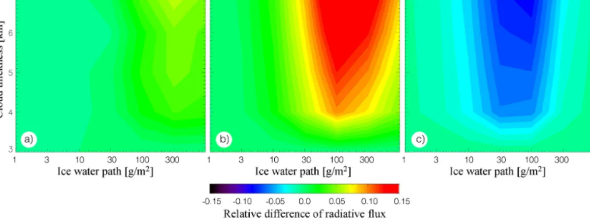
Figure 8. The relative difference in calculated TOA_LW fluxes with respect to rectangular IWC(z) profile type estimated for 3 to 7 km thick clouds with average De = 50 µm (kAB=1.5, see Sect. 3.3) and with a cloud top at 15 km: (a) isosceles trapezoid; (b) lower triangles;
(c) upper triangles.
4.2.2 Relative differences in LW radiative fluxes
As we have seen before, in 75 % of all high ice clouds one can approximate the IWC profile by a rectangular or isosceles trapezoid shape. For the rest of the cases, however, we want to estimate the radiative impact of using a “realistic” (DAR-DAR) IWC profile instead of a constant IWC profile and see how much this will affect the difference in fluxes at the TOA, SRF and atmosphere (ATM). Correspondingly, we compare SRF, TOA, and ATM values for each combination of IWP,
z, De, and 1z for three IWC profile types vs. the results ob-tained with a rectangular profile. Figure 8 shows a represen-tative example of such a comparison for the TOA_LW flux differences built for the three IWC profile shapes vs. rectan-gular one. For these plots, 1zcldvaried from 3 to 7 km, and
IWP varied from 1 to 1000 g m−2. As one can see, the radia-tive effects of the isosceles trapezoid type (Fig. 8a) are almost identical to that of the rectangular type. On the other hand, there are noticeable effects in TOA_LW fluxes for lower and upper triangle IWC profile types (Fig. 8b, c) for 1z larger than 3 km and IWP larger than 30 g m−2.
We explain the observed differences by the nature of the LW cloud radiance: the LW fluxes are composed of terres-trial, atmospheric, and cloud components. The terrestrial and atmospheric radiances originating below the cloud are ab-sorbed by clouds with the same IWP in the same way. The atmospheric radiance above the cloud is the same in all com-pared cases. However, the emitted cloud radiance depends on the shape of the IWC profile: temperature in the tropo-sphere decreases with height, so the effective altitude of the upper and lower triangles will differ from that of the cloud with a constant IWC. Correspondingly, the lower triangle type cloud will emit more radiance than the rectangular type, which, in turn, will emit more than the upper triangle type. As for the trapezoid, its effective radiative height is about the same as that of the rectangular-type cloud. The magnitude
of the effect (Fig. 8b, c) increases with 1z since the dif-ference between kinetic temperatures of effective radiative cloud layer increases. However, for optically thick clouds (see large IWP values in the right-hand side of Fig. 8b, c panels) the effect washes out since high optical thickness “moves” the effective radiative heights upwards, making the differences between them smaller. The same considerations apply for the SRF_LW fluxes (not shown), but in this case at-mospheric absorption and emission in the thick lower atmo-sphere mask the changes and the differences are smaller than 1 %. Adding optically thick water cloud underneath the ice cloud does not significantly change either of the conclusions made above: TOA_LW is still modulated by the effective ra-diative height, while the surface becomes more isolated from the ice cloud, further reducing the sensitivity of SRF_LW to IWC(z).
4.2.3 Relative differences in SW radiative fluxes
In a similar manner, we have analyzed the sensitivity of SW fluxes to IWC profile type (Fig. 9). The effects in TOA_SW are opposite to those in TOA_LW (Fig. 8): the radiance es-caping the atmosphere is smaller in the case of lower tri-angle IWC(z) compared to the cloud of a rectangular type. The study shows that this effect is related to the De pro-file. Small and large particles scatter solar radiance differ-ently. Correspondingly, convolving De(z), which increases towards the cloud base (see Sect. 3.3 and Fig. 6), with the IWC profiles of a different type changes the amount of ra-diance scattered backwards. To justify this explanation, we have performed a test with a constant De within the cloud layer (not shown), which reduced the differences in Fig. 9a–c to less than 1 %. The same mechanism and explanation apply to SRF_SW fluxes differences in Fig. 9d–f, where the effects are the opposite to that in TOA_SW: lower triangles cause larger SRF_SW than rectangular type IWC profiles in thick clouds. As for the TOA_SW, the effect is gone if a constant
Figure 9. The relative difference in SW fluxes with respect to rectangular IWC(z) profile type estimated for 3 to 7 km thick clouds with average De = 50 µm and with a cloud top at 15 km. (a–c) TOA; (d–f): SRF; (a, d) isosceles trapezoid; (b, e) lower triangles; (c, f) upper triangles.
De is used. Both the TOA_SW and SRF_SW fluxes show weak sensitivity to substituting rectangular IWC profile with trapezoid one due to an obvious reason: the contributions of particles with De significantly different from the average De in the cloud layer are reduced by IWC(z) profile. Adding a water cloud beneath the ice cloud reduces the effects in TOA_SW for the IWP values less than 50 g m−2. This is due to a contribution of the water cloud to the TOA_SW flux: a part of solar radiance, which has passed through an ice cloud, is reflected back, increasing the TOA_SW and washing out the effects of the ice cloud itself. As for the SRF_SW in the case of an underlying water cloud, the sensitivity of the flux to the IWC profile change reduces by a factor of ∼ 2 because of the absorption in the water cloud.
4.2.4 Absolute differences of
IWC-profile-shape-weighted SW and LW fluxes
Even though some of the panels in Figs. 8 and 9 show notice-able changes in TOA and SRF fluxes, this knowledge alone is not enough to estimate the energetic effects of using the rectangular type IWC(z) in all the cases instead of using real (or more realistic) profiles. To do that, we have used a pre-calculated set of 98 000 fluxes as a big lookup table (LUT) (see Sect. 4.2.1) and applied it to each of the events in the collocated data set. For clear-sky cases, we used a corre-sponding clear-sky profile to obtain realistic cloud-amount-weighted fluxes (we used cloud amount from AIRS). For
cloudy cases, we used the fluxes corresponding to the best fit IWC model profile (if the best fit returned the rectangular profile it was included to keep the statistics unbiased). In Ta-ble 6, we compare net SW + LW fluxes at the TOA, SRF, and their difference, ATM, averaged for both approaches. The table contains net flux differences estimated, separately for single-layer high clouds and for all scenes, including mul-tiple layer clouds and clear sky cases. Correspondingly, the first part can be used for estimating the average radiative ef-fects in the cloudy cases, while the second part represents high ice cloud-amount-weighted differences in fluxes acting globally.
Obviously, the LUTs we have used to make these estimates cannot cover all possible permutations of ice clouds and wa-ter clouds of variable optical depth at different distances from the ice clouds, not speaking about different water and ice particle size distributions, but the values in Table 6 give an estimate of the significance of the effect. The sign and mag-nitude of the values are related to an interplay between the effects in the ratios of the fluxes considered in Sect. 4.2.2. and 4.2.3 convolved with the occurrence frequencies of dif-ferent IWC profile shapes and with occurrence frequencies of corresponding IWPs, cloud top heights, and 1z. We high-light several features. From the comparison of TOA_LW and TOA_SW flux sensitivity (Figs. 8 and 9a–c), one can see that SW and LW flux responses are in a counter-phase: us-ing lower triangle instead of constant IWC profile increases
Table 6. Differences in radiative fluxes for July: real IWC(z) profiles vs. constant IWC(z), supplemented with interannual variability for 2007–2009 (values in brackets). Global average is area weighted.
Only single-layer high cloud scenes Cloud amount weighted
Atm. TOA SRF ATM TOA SRF ATM
type [W m−2] [W m−2] [W m−2] [W m−2] [W m−2] [W m−2] SAW −0.03 ± 0.04 −2.08 ± 0.08 2.05 ± 0.05 0.00 ± 0.01 −0.31 ± 0.01 0.32 ± 0.01 MLW 0.92 ± 0.02 −1.96 ± 0.04 2.89 ± 0.06 0.16 ± 0.00 −0.35 ± 0.01 0.52 ± 0.01 TROP 1.07 ± 0.02 −1.10 ± 0.06 2.17 ± 0.08 0.27 ± 0.01 −0.28 ± 0.02 0.56 ± 0.02 MLS 2.06 ± 0.07 −2.17 ± 0.14 4.23 ± 0.21 0.49 ± 0.03 −0.49 ± 0.04 0.98 ± 0.06 SAS 1.63 ± 0.08 −2.66 ± 0.12 4.29 ± 0.19 0.20 ± 0.02 −0.32 ± 0.03 0.51 ± 0.05 Glob. avg. 1.25 ± 0.02 −1.68 ± 0.06 2.93 ± 0.08 0.24 ± 0.01 −0.38 ± 0.01 0.62 ± 0.01
LW flux, but decreases SW flux. As discussed above, a cloud underlying the ice cloud reduces the surface radiative effect both in SW and in LW. Small TOA values for the SAW (sub-arctic winter type) atmosphere are linked to polar night con-ditions and associated with a lack of both reflected solar radi-ance and high level ice clouds on the poles. Cloud-amount-weighted net flux differences are significantly smaller than those estimated for only cloudy cases: all values in the sec-ond part of Table 6 are smaller than 1 W m−2, while the ATM flux differences in the first part reach ∼ 4 W m−2and TOA and SRF net flux differences reach ∼ 2 W m−2. These esti-mates should be supplemented by differences related to IWC profile shapes in low thick ice clouds as well as to LWC (liq-uid water content) profiles in water clouds that can be a sub-ject of a separate study. However, the vertical extent of these clouds is much smaller compared to that of high clouds, so the radiative effects are expected to be smaller, too.
5 Conclusion
Since IR sounders only determine bulk cirrus microphysical properties, we added the data from active instruments to get a deeper insight into vertical profiles of IWC and De. The primary object of this analysis was to find out if the IWC profiles can be classified according to simple shapes, ideally as a function of parameters determined by IR sounders alone, and to determine the effect on the radiative properties of the cloud. Below we list the most important findings of our anal-yses.
1. A minimal and sufficient set of primitive shapes rep-resenting the IWC profiles in high ice clouds consists of four elements: rectangular, isosceles trapezoid, up-per triangle, and lower triangle. The statistical analysis shows that rectangular and trapezoid IWC shapes to-gether make up more than 70 % of all the cases with trapezoid-like IWC profiles dominating both single- and multi-layer scenes. The fraction of lower triangles in-creases with IWP, reaching 33 % for IWP > 300 g m−2. The fraction of upper triangles is 19 % for multi-layer
scenes at IWP < 10 g m−2and decreases with IWP in-crease.
2. The main variable, which should be used for the IWC profile shape statistical classification is IWP. Cloud ver-tical extent strongly correlates with a logarithm of IWP, land/ocean distributions demonstrate similar behaviour, and latitudinal variability of the most frequent shape is moderate. However, the dependence of the profile shape on IWP is strong, consistent with the current under-standing of cirrus formation physics. Single-layer high clouds and multi-layer scenes demonstrate qualitatively similar behaviour, but the relative occurrence of lower triangle shapes is slightly larger for the former and the relative occurrence of upper triangle shapes is slightly larger for the latter. We have observed a correlation be-tween the lower triangle fraction and strong downdrafts within the cloud (wcloud>175 hPa day−1), leading to
3–11 % anomalies (up to 50 % relative change).
3. The effective ice crystal diameter of high ice clouds in general increases towards cloud base (i.e. Heymsfield and Iaquinta, 2000). We found that its vertical profile can be parameterized by a trapezoid shape. The ratio of its lower and upper edges is 1.1 for IWP < 10 g m−2and 1.35–1.5 for IWP > 50 g m−2.
4. We have estimated the radiative effects of clouds with the same IWP but with different IWC profile shape for five typical atmospheric scenarios and over a broad range of IWP, cloud height, cloud thickness, and De values. In this analysis, lower , upper triangle-and trapezoid- IWC profiles were compared to a “refer-ence” rectangular profile. We explain the observed dif-ferences in TOA_LW fluxes by thermal radiance of the cloud and by changes of the “effective radiative layer” height depending on the IWC profile. The differences in TOA_SW fluxes are related to De vertical profiles: changing the IWC profile shape leads to a different ef-fective value of De that, in turn, leads to different scat-tering characteristics of the cloud. Adding a thick water
Appendix A
Table A1. Abbreviations.
AIRS Atmospheric Infrared Radiation Spectrometer AMSU Advanced Microwave Sounding Unit
ATM Atmosphere
CALIOP Cloud-Aerosol Lidar with Orthogonal Polarization
CALIPSO Cloud Aerosol Lidar and Infrared Pathfinder Satellite Observation DARDAR raDAR/liDAR
DISORT Discrete Ordinates Radiative Transfer
ECMWF European Centre for Medium-Range Weather Forecasts ERA ECMWF’s re-analysis
GEOPROF Geometric profiling
IASI Infrared Atmospheric Sounding Interferometer
IR Infrared
IWC Ice water content LBLRTM Line-by-line RRTM
LMD Laboratory of Dynamic Meteorology
LT Local time
LUT Lookup table
LW Long wave
LWC Liquid water content
MLS Midlatitude summer type atmosphere MLW Midlatitude winter type atmosphere
MODIS Moderate Resolution Imaging Spectroradiometer NOAA National Oceanic and Atmospheric Administration RRTM Rapid Radiative Transfer Model
SAS Subarctic summer type atmosphere SAW Subarctic winter type atmosphere SRF Surface radiative flux
SW Short wave
TOA Top of atmosphere
TOVS TIROS Operational Vertical Sounder TROP Tropical type atmosphere
References
Bardeen, C. G., Gettelman, A., Jensen, E. J., Heymsfield, A., Con-ley, A. J., Delanoë, J., Deng, M., and Toon, O. B.: Improved cir-rus simulations in a general circulation model using CARMA sectional microphysics, J. Geophys. Res.-Atmos., 118, 11679– 11697, 2013.
Battaglia, A. and Delanoë, J.: Synergies and complementarities of CloudSat-CALIPSO snow observations, J. Geophys. Res., 118, 721–731, 2013.
Bony, S. and Dufresne, J.-L.: Marine boundary layer clouds at the heart of cloud feedback uncertainties in climate models, Geo-phys. Res. Lett., 32, L20806, doi:10.1029/2005GL023851, 2005. Ceccaldi, M., Delanoë, J., Hogan, R. J., Pounder, N. L., Protat, A., and Pelon, J.: From CloudSat-CALIPSO to EarthCare: Evolu-tion of the DARDAR cloud classificaEvolu-tion and its comparison to airborne radar-lidar observations, J. Geophys. Res., 118, 7962– 7981, doi:10.1002/jgrd.50579, 2013.
Chahine, M., Pagano, T., T. S., Aumann, H. H., Atlas, R., Barnet, C., Blaisdell, J., Chen, L., Divakarla, M., Fetzer, E. J., Gold-berg, M., Gautier, C., Granger, S., Hannon, S., Irion, F. W., Kakar, R., Kalnay, E., Lambrigtsen, B. H., Lee, S.-Y., Le Mar-shall, J., McMillan, W. W., McMillin, L., Olsen, E. T., Rever-comb, H., Rosenkranz, P., Smith, W. L., Staelin, D., Strow, L. L., Susskind, J., Tobin, D., Wolf, W., and Zhou, L.: AIRS: improv-ing weather forecastimprov-ing and providimprov-ing new data on greenhouse gases, B. Am. Meteorol. Soc., 87, 911–926, doi:10.1175/BAMS-87-7-911, 2006.
Chalon, G., Cayla, F., and Diebel, D.: IASI: an advanced sounder for operational meteorology, in: Proceedings of the 52nd Congress of IAF, 1–5 October 2001, Toulouse, France, 2001.
Clough, S. A., Shephard, M. W., Mlawer, E. J., Delamere, J. S., Iacono, M. J., Cady-Pereira, K., Boukabara, S., and Brown, P. D.: Atmospheric radiative transfer modeling: a summary of the AER codes, Short Communication, J. Quant. Spectrosc. Ra., 91, 233–244, 2005.
Davis, S., Hlavka, D., Jensen, E., Rosenlof, K., Yang, Q., Schmidt, S., Borrmann, S., Frey, W., Lawson, P., Voemel, H., and Bui, T. P.: In situ and lidar observations of tropopause subvisi-ble cirrus clouds during TC4, J. Geophys. Res., 115, D00J17, doi:10.1029/2009JD013093, 2010.
Dee, D. P., Uppala, S. M., Simmons, A. J., Berrisford, P., Poli, P., Kobayashi, S., Andrae, U., Balmaseda, M. A., Balsamo, G., Bauer, P., Bechtold, P., Beljaars, A. C. M., van de Berg, L., Bid-lot, J., Bormann, N., Delsol, C., Dragani, R., Fuentes, M., Geer,
Delanoë, J., Hogan, R. J., Forbes, R. M., Bodas-Salcedo, A., and Stein, T. H. M.: Evaluation of ice cloud representation in the ECMWF and UK Met Office models using CloudSat and CALIPSO data, Q. J. Roy. Meteor. Soc., 137, 2064–2078, 2011. Delanoë, J., Protat, A., Jourdan, O., Pelon, J., Papazzoni, M., Dupuy, R., Gayet, J.-F., and Jouan, C.: Comparison of airborne in-situ, airborne radar-lidar, and spaceborne radar-lidar retrievals of polar ice cloud properties sampled during the POLARCAT campaign, J. Atmos. Ocean. Tech., 30, 57–73, 2013.
Deng, M., Mace, G. G., Wang, Z., and Lawson, R. P.: Evaluation of several A-Train ice cloud retrieval products with in situ measure-ments collected during the SPartICus campaign, J. Appl. Me-teorol. Clim., 52, 1014–1030, doi:10.1175/JAMC-D-12-054.1, 2013.
Eliasson, S., Buehler, S. A., Milz, M., Eriksson, P., and John, V. O.: Assessing observed and modelled spatial distributions of ice water path using satellite data, Atmos. Chem. Phys., 11, 375– 391, doi:10.5194/acp-11-375-2011, 2011.
Eliasson, S., Holl, G., Buehler, S. A. A., Kuhn, T., Stengel, M., Iturbide-Sanchez, F., and Johnston, M.: Systematic and random errors between collocated satellite ice water path observations, J. Geophys. Res., 2629–2642, doi:10.1029/2012JD018381, 2012. Faijan, F., Lavanant, L., and Rabier, F.: Towards the use
of cloud microphysical properties to simulate IASI spectra in an operational context, J. Geophys. Res., 117, D22205, doi:10.1029/2012JD017962, 2012.
Feofilov, A. G. and Kutepov, A. A.: Infrared Radiation in the Meso-sphere and Lower ThermoMeso-sphere: Energetic Effects and Remote Sensing, Surv. Geophys., 33, 1231–1280, doi:10.1007/s10712-012-9204-0, 2012.
Fu, Q.: An accurate parameterization of the solar radiative prop-erties of cirrus clouds for climate models, J. Climate, 9, 2058– 2082, 1996.
Gayet, J.-F., Shcherbakov, V., Bugliaro, L., Protat, A., Delanoë, J., Pelon, J., and Garnier, A.: Microphysical properties and high ice water content in continental and oceanic mesoscale convective systems and potential implications for commercial aircraft at flight altitude, Atmos. Chem. Phys., 14, 899–912, doi:10.5194/acp-14-899-2014, 2014.
Guignard, A., Stubenrauch, C. J., Baran, A. J., and Armante, R.: Bulk microphysical properties of semi-transparent cirrus from AIRS: a six year global climatology and statistical anal-ysis in synergy with geometrical profiling data from CloudSat-CALIPSO, Atmos. Chem. Phys., 12, 503–525, doi:10.5194/acp-12-503-2012, 2012.
Haladay, T. and Stephens, G.: Characteristics of tropical thin cirrus clouds deduced from joint CloudSat and CALIPSO observations, J. Geophys. Res., 114, D00A25, doi:10.1029/2008JD010675, 2009.
Haynes, J. M. and G. L. Stephens, G. L.: Tropical oceanic cloudiness and the incidence of precipitation: Early re-sults from CloudSat, Geophys. Res. Lett., 34, L09811, doi:10.1029/2007GL029335, 2007.
Heymsfield, A. J. and Iaquinta, J.: Cirrus crystal terminal velocities, J. Atmos. Sci., 57, 916–938, 2000.
Hilton, F., Armante, R., August, T., Barnet, C., Bouchard, A., Camy-Peyret, C., Capelle, V., Clarisse, L., Clerbaux, C., Co-heur, P.-F., Collard, A., Crevoisier, C., Dufour, G., Edwards, D., Faijan, F., Fourrié, N., Gambacorta, A., Goldberg, M., Guidard, V., Hurtmans, D., Illingworth, S., Jacquinet-Husson, N., Kerzen-macher, T., Klaes, D., Lavanant, L., Masiello, G., Matricardi, M., McNally, A., Newman, S., Paveli, E., Payan, S., Péquignot, E., Peyridieu, S., Phulpin, T., Remedios, J., Schlüssel, P., Se-rio, C., Strow, L., Stubenrauch, C. J., Taylor, J., Tobin, D., Wolf, W., and Zhou, D.: Hyperspectral Earth Observation from IASI, B. Am. Meteorol. Soc., 93, 347–370, doi:10.1175/BAMS-D-11-00027.1, 2012.
Holz, R., Ackerman, S. A., Antonelli, P., Nagle, F., Knuteson, R. O., McGill, M., Hlavka, D. L., and Hart, W. D.: An Improvement to the High Spectral Resolution CO2Slicing Cloud Top Altitude
Retrieval, J. Atmos. Ocean. Technol., 23, 653–670, 2008. Hu, Y., Vaughan, M., Liu, Z., Lin, B., Yang, P., Flittner, D., Hunt,
B., Kuehn, R., Huang, J., Wu, D., Rodier, S., Powell, K., Trepte, C., and Winker, D.: The depolarization–attenuated backscatter relation: CALIPSO lidar measurements vs. theory, Opt. Express, 15, 5327–5332, 2007.
Hu, Y. X. and Stamnes, K.: An accurate parameterization of the radiative properties of water clouds suitable for use in climate models, J. Climate, 6, 728–742, 1993.
Huang, Y., Siems, S. T., Manton, M. J., Protat, A., and Delanoë, J.: A study on the low-altitude clouds over the Southern Ocean using the DARDAR-MASK, J. Geophys. Res., 117, D18204, doi:10.1029/2012JD017800, 2012.
Iacono, M. J., Mlawer, E. J., Clough, S. A., and Morcrette, J.-J.: Impact of an improved long-wave radiation model RRTM on the energy budget and thermodynamic properties of the NCAR community climate mode, CCM3, J. Geophys. Res., 105, 14873– 14890, 2000.
Jouan, C., Girard, E., Pelon, J., Gultepe, I., Delanoë, J., and Blanchet, J.-P.: Characterization of Arctic ice cloud proper-ties observed during ISDAC, J. Geophys. Res., 117, D23207, doi:10.1029/2012JD017889, 2012.
Jouan, C., Pelon, J., Girard, E., Ancellet, G., Blanchet, J. P., and Delanoë, J.: On the relationship between Arctic ice clouds and polluted air masses over the North Slope of Alaska in April 2008, Atmos. Chem. Phys., 14, 1205–1224, doi:10.5194/acp-14-1205-2014, 2014.
Kärcher, B. and Lohmann, U.: A parameterization of cir-rus cloud formation: Homogenous freezing of super-cooled aerosols, J. Geophys. Res., 107, AAC4.1–AAC4.10, doi:10.1029/2001JD000470, 2002
Key, J. and Schweiger, A. J.: Tools for atmospheric radiative trans-fer: Streamer and FluxNet, Comput. Geosci., 24, 443–451, 1998.
Kienast-Sjögren, E., Spichtinger, P., and Gierens, K.: Formulation and test of an ice aggregation scheme for two-moment bulk microphysics schemes, Atmos. Chem. Phys., 13, 9021–9037, doi:10.5194/acp-13-9021-2013, 2013.
Liao, X., Rossow, W. B., and Rind, D.: Comparison between SAGE II and ISCCP high level clouds, Part II: Locating cloud tops, J. Geophys. Res., 100, 1137–1147, 1995.
Mace, G. G., Zhang, Q., Vaughan, M., Marchand, R., Stephens, G., Trepte, C., and Winker, D.: A description of hydrometeor layer occurrence statistics derived from the first year of merged Cloudsat and CALIPSO data, J. Geophys. Res., 114, D00A26, doi:10.1029/2007JD009755, 2009
Martins, E., Noel, V., and Chepfer, H.: Properties of cirrus and subvisible cirrus from nighttime Cloud-Aerosol Lidar with Or-thogonal Polarization (CALIOP), related to atmospheric dy-namics and water vapor, J. Geophys. Res., 116, D02208, doi:10.1029/2010JD014519, 2011.
Mason, S., Jakob, C., Protat, A., and Delanoë, J.: Characterising observed mid-topped cloud regimes associated with Southern Ocean shortwave radiation biases, J. Climate, 27, 6189–6203, 2014.
Mlawer, E. J. and Clough, S. A.: On the extension of rapid radia-tive transfer model to the shortwave region, in Proceedings of the 6th Atmospheric Radiation Measurement (ARM) Science Team Meeting, US Department of Energy, CONF-9603149, 1997. Mlawer, E. J. and Clough, S. A.: Shortwave and long-wave
enhance-ments in the rapid radiative transfer model, in Proceedings of the 7th Atmospheric Radiation Measurement (ARM) Science Team Meeting, US Department of Energy, CONF-970365, 1998. Mlawer, E. J., Taubman, S. J., Brown, P. D., Iacono, M. J., and
Clough, S. A.: Radiative transfer for inhomogeneous atmo-spheres: RRTM, a validated correlated-k model for the long-wave, J. Geophys. Res., 102, 16663–16682, 1997.
Morcrette, J.-J.: Impact of the radiation-transfer scheme RRTM in the ECMWF forecasting system, ECMWF Newsletter No. 91, 2001.
Oreopoulos, L., Mlawer, E., Delamere, J., Shippert, T., Cole, J., Fomin, B., Iacono, M., Jin, Z., Li, J., Manners, J., Räisänen, P., Rose, F., Zhang, Y., Wilson, M. J., and Rossow, W. B.: The con-tinual intercomparison of radiation codes: results from phase I, J. Geophys. Res., 117, D06118, doi:10.1029/2011JD016821, 2012. Smith, W. L., Woolf, H. M., Hayden, C. M., Wark, D. C., and McMillin, L. M.: TIROS-N operational vertical sounder, B. Am. Meteorol. Soc., 60, 1177–1187, 1979.
Stamnes, K., Tsay, S. C., Wiscombe, W., and Jayaweera, K.: Nu-merically stable algorithm for discrete-ordinate-method radiative transfer in multiple scattering and emitting layered media, Appl. Optics, 27, 2502–2509, 1988.
Stein, T. H. M., Parker, D. J., Delanoë, J., Dixon, N. S., Hogan, R. J., Knippertz, P., Maidment, R. I., and Marsham, J. H.: The vertical cloud structure of the West African monsoon: A 4 year climatology using CloudSat and CALIPSO, J. Geophys. Res., 116, D22205, doi:10.1029/2011JD016029, 2011a.
Stein, T. H. M., Delanoë, J., and Hogan, R. J.: A comparison be-tween different retrieval methods for ice cloud properties using data from the CloudSat and A-Train satellites, J. Appl. Meteorol. Clim., 50, 1952–1969, 2011b.
Stephens, G. L., Vane, D. G., Boain, R. J., Mace, G. G., Sassen, K., Wang, Z., Illingworth, A. J., O’Connor, E. J., Rossow, W.
rar, S.: Cloud properties and their seasonal and diurnal variability from TOVS Path-B, J. Climate, 19, 5531–5553, 2006.
Stubenrauch, C. J., Cros, S., Lamquin, N., Armante, R., Chédin, A., Crevoisier, C., and Scott, N. A.: Cloud properties from AIRS and evaluation with CALIPSO, J. Geophys. Res., 113, D00A10, doi:10.1029/2008JD009928, 2008.
Stubenrauch, C. J., Cros, S., Guignard, A., and Lamquin, N.: A 6-year global cloud climatology from the Atmospheric In-fraRed Sounder AIRS and a statistical analysis in synergy with CALIPSO and CloudSat, Atmos. Chem. Phys., 10, 7197–7214, doi:10.5194/acp-10-7197-2010, 2010.
Stubenrauch, C. J., Rossow, W. B., Kinne, S., Ackerman, S., Ce-sana, G., Chepfer, H., Di Girolamo, L., Getzewich, B., Guig-nard, A., Heidinger, A., Maddux, B. C., Menzel, W. P., Minnis, P., Pearl, C., Platnick, S., Poulsen, C., Riedi, J., Sun-Mack, S., Walther, A., Winker, D., Zeng, S., and Zhao, G.: Assessment of global cloud datasets from satellites: Project and Database initi-ated by the GEWEX Radiation Panel, B. Am. Meteorol. Soc., 94, 1031–1049, doi:10.1175/BAMS-D-12-00117, 2013.
Technol., 26, 2034–2050, 2009.
Wylie, D., Jackson, D. L., Menzel, W. P., and Bates, J. J.: Trends in Global Cloud Cover in Two Decades of HIRS Observations, J. Climate, 18, 3021–3031, 2005.
Winker, D. M., Pelon, J., and McCormick, M. P.: The CALIPSO mission: Spaceborne lidar for observation of aerosols and clouds, Proc. SPIE Int. Soc. Opt. Eng., 4893, 1–11, 2003.