HAL Id: hal-00318015
https://hal.archives-ouvertes.fr/hal-00318015
Submitted on 30 Nov 2005
HAL is a multi-disciplinary open access
archive for the deposit and dissemination of
sci-entific research documents, whether they are
pub-lished or not. The documents may come from
teaching and research institutions in France or
abroad, or from public or private research centers.
L’archive ouverte pluridisciplinaire HAL, est
destinée au dépôt et à la diffusion de documents
scientifiques de niveau recherche, publiés ou non,
émanant des établissements d’enseignement et de
recherche français ou étrangers, des laboratoires
publics ou privés.
physical-biogeochemical model using partially-local
Kalman filters
I. Hoteit, G. Triantafyllou, G. Petihakis
To cite this version:
I. Hoteit, G. Triantafyllou, G. Petihakis. Efficient data assimilation into a complex, 3-D
physical-biogeochemical model using partially-local Kalman filters. Annales Geophysicae, European
Geo-sciences Union, 2005, 23 (10), pp.3171-3185. �hal-00318015�
SRef-ID: 1432-0576/ag/2005-23-3171 © European Geosciences Union 2005
Annales
Geophysicae
Efficient data assimilation into a complex, 3-D
physical-biogeochemical model using partially-local Kalman filters
I. Hoteit1, G. Triantafyllou2, and G. Petihakis2
1Scripps Institution of Oceanography, La Jolla, CA, USA 2Hellenic Centre for Marine Research, Anavissos, Greece
Received: 1 December 2004 – Revised: 11 August 2005 – Accepted: 9 September 2005 – Published: 30 November 2005
Abstract. Advanced Kalman filtering techniques were
used to assimilate pseudo ocean color and profile data into a complex, three-dimensional coupled physical (POM)-biogeochemical (ERSEM) model of the Cretan Sea ecosys-tem. The assimilation schemes, the Singular Evolutive Partially-Local Extended Kalman (SEPLEK) filter and its variant called SFPLEK, are based on the standard SEEK fil-ter in which the Kalman correction is made along a set of “global” and “local” directions, determined via a so-called “global-local EOF analysis”. The global functions are used to represent the ecosystem large-scale variability. They are allowed to evolve in time in the SEPLEK filter to follow changes in the model dynamics, while they remain invari-ant in the SFPLEK filter. The local functions always remain invariant and are determined in such a way as to indepen-dently represent the different spatial regimes of the ecolog-ical model. This helps to improve the estimation of fine-scale variations while requiring significantly less computa-tional time compared to the SEEK filter.
Several assimilation experiments were performed to as-sess the relevance of the assimilation system and to study its sensitivity to different choices of global/local EOFs. The SFPLEK filter was used in all the sensitivity experiments in order to efficiently measure the representativeness of the dif-ferent set of correction directions, as well as to save com-putational time. Assimilation results suggest that the use of global-local correction directions clearly enhances the filter’s performance under different assimilation setups. The choice of the local directions should, however, be carefully consid-ered, taking into account the model regional variability and the characteristics of the observational system.
Keywords. Oceanography: General (numerical modeling;
Ocean prediction) – Biological and Chemical (ecosystems and ecology)
Correspondence to: G. Triantafyllou
1 Introduction
The Cretan Sea is located in the northwest part of the eastern Mediterranean Sea. It is linked with the Levantine basin and the Ionian Sea through the eastern and western straits of the Cretan Arc. The area is dominated by multiple scale circu-lation patterns with a complex hydrological structure charac-terized by mesoscale variability. As described in a 3-D mod-eling study of the Cretan Sea (Petihakis et al., 2002) the cy-clonic circulation to the north of the central and eastern part of the island, in conjunction with the anticyclonic circulation in the north central part, results in areas of increased produc-tion around the cyclone, in contrast to the area affected by the anticyclonic activity. The system is characterized by a seasonal thermocline (60–80 m) from spring to autumn, sep-arating the water column into two layers. Primary and bac-terial production decrease moving offshore while increased production rates are associated with intense mixing events and the subsequent nutrient intrusion to the euphotic zone. Thus most of the primary production in the euphotic zone is supported by regenerated nutrients. As in all complex sys-tems, advanced numerical models seem to be the only op-tion for the simulaop-tion of the behavior and the evoluop-tion of the Cretan Sea ecosystem (see Thingstad et al., 1999). Such models, however, include a significant number of parameters which are usually provided by the scientific literature, having been derived through laboratory experiments and in-situ ob-servations of a similar type ecosystem. To advance beyond this subjective approach, data assimilation is the process of finding the model solution which is most consistent with the observations. These techniques are essential in producing the most complete picture of the system by integrating all avail-able knowledges, including observations (in-situ and satellite data) and biophysical principles (state-of-the-art numerical models).
Data assimilation methods can be classified into two cate-gories: variational methods based on the optimal control the-ory and sequential methods based on the statistical estimation theory (see Malanotte-Rizzoli, 1996). Variational methods
have been considered by a number of studies (Evans, 1999; Matear, 1995; Harmon and Challenor, 1996). For instance, Lawson et al. (1996) used the well-known adjoint method with a simple ecosystem model. The same method has re-cently been efficiently implemented by Faugeras et al. (2003) to assimilate chlorophyll data into a 1-D ecosystem model. Relying on the assumption that a coupled model with a given set of parameters can reproduce the observations, variational methods can be strongly sensitive to the unresolved processes of the model formulation. Although model error can be in principle, considered by applying a weak constraint inverse formulation (Natvik et al., 2001), this would make the dimen-sion of the search so long that unpreconditioned searches for a best fit would be prohibitive. Sequential methods which al-low one to incorporate the model error seem, therefore, to be more appropriate for data assimilation into marine ecosystem models.
The application of sequential methods for data assimila-tion into ecosystem models has received more attenassimila-tion dur-ing the last decade. These techniques are generally derived from the extended Kalman (EK) filter. Indeed, the implemen-tation of the EK filter in realistic ocean models is not possible because of its prohibitive computational burden. Different simplified forms of this filter have therefore been developed, basically reducing the dimension of the system through some kind of projection onto a low dimensional subspace (Cane et al., 1995; Fukumori and Malanotte-Rizzoli, 1995; Verlaan and Heemink, 1995). Recently, Monte Carlo techniques were also introduced to avoid the linearization of the model equa-tions, leading to the ensemble Kalman methods (Evensen and van Leeuwen, 1994; Burgers et al., 1998). Allen et al. (2003) and Natvik and Evensen (2003) demonstrated the effective-ness of the ensemble Kalman filter for data assimilation with a 1-D, three-component ecosystem model.
The singular evolutive extended Kalman (SEEK) filter is a simplified square-root EK filter which has been introduced by Pham et al. (1998). It basically makes use of singular, low-rank matrices approximations of the filter’s error covari-ance matrix. This leads to the application of the Kalman’s correction only along the directions for which the forecast er-ror was not sufficiently attenuated by the system. The SEEK filter has been successfully implemented in several marine ecosystem models. Carmillet et al. (2001) assimilated ocean color data with a 3-D biophysical model of the north Atlantic Ocean, while keeping the correction directions invariant in time to reduce computational time (called hereafter the Sin-gular fixed extended Kalman (SFEK) filter). The same filter has also been used by Hoteit et al. (2003) to assimilate real Oxygen and Nitrate data into a 1-D ecosystem model. The behavior of this filter can, however, be degraded in the pres-ence of model instabilities, generally not well represented by an invariant set of correction directions (Hoteit et al., 2002). A further extension of the 1-D to a 3-D system has been pre-sented by Triantafyllou et al. (2003a) with the first applica-tion of an advanced Kalman filtering technique (ensemble variant of the SEEK filter, called SEIK filter) for data assim-ilation into a complex, three-dimensional marine ecosystem
model. In the latter work, however, the number of directions was limited by the available computational resources.
Limits in computer capacity further complicate the estima-tion of short-range phenomena with Kalman filtering tech-niques, generally inefficient when dealing with such intermit-tent processes (Bennett, 1992). This makes the data assimi-lation into marine ecosystem models particularly difficult be-cause an important part of the variability of these models is governed by fine-scale variations. In this study, the Semi-Evolutive Partially-Local Extended Kalman (SEPLEK) was used to tackle these problems. This filter was found to be more performant than the SEEK filter when dealing with variables having short-range variability, while requiring sig-nificantly less computational time (Hoteit et al., 2001). This is possible due to the ability of adapting the correction di-rections of this filter to the different spatial regimes of the system under study. Specifically, global and local functions are used to better represent the long-range and the differ-ent short-range variability of the model, using a so-called “global-local” Empirical Orthogonal Functions (EOF) analy-sis. Only the global functions are allowed to evolve in time to follow changes in the model dynamics, while the local func-tions remain invariant. This significantly reduces the compu-tational burden compared to the SEEK filter, as the number of required global functions is generally small. Additional cost reduction can be further obtained by keeping the global functions invariant, which also provides the best way to as-sess the representativeness of a given set of correction direc-tions (Brasseur et al., 1999). This simplified variant of the SEPLEK filter was, therefore, used in our sensitivity exper-iments. It has the same algorithm as the SFEK filter, but makes use of partially local correction directions. Hence, it will be called the Singular Fixed Partially Local Extended Kalman (SFPLEK) filter, in order to remove any confusion with the (classical) SFEK filter which was also considered in this study. Note that, although this study is closely related to that of Triantafyllou et al. (2003a) mentioned above, since the same ecosystem model was used in both studies, the re-sults of this work were not linked to the latter, in order to avoid a complex comparison between an ensemble filter and a partially-local extended filter. It is actually more appropri-ate to carry out this comparison using a local variant of the SEIK filter, which can be developed in a similar way to the local Ensemble Kalman filter (Ott et al., 2004). This will be one of our future objectives. In this study, however, we de-cided to only focus on the evaluation of the benefits of using local EOFs in an ecological assimilation system.
Numerical experiments were performed to assess the rel-evance of the assimilation system and to study its sensitiv-ity to different parameters and setups. An important part of this work is devoted to studying the impact of the choice of local EOFs on the performance of the filter. For instance, Carmillet et al. (2001) already tested the idea of separating the euphotic zone from the deep ocean by excluding the deep ocean variables from the state vector of the filter. This idea is further extended here while representing these two different regimes, using independent (vertical) local functions instead
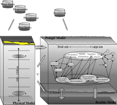
Wind Stress Evaporation Precipitation Heat fluxes Irradiation Physical Model 100 - 1500 m Benthic Model Particulate Si NH4 N PO4 NO3 Pelagic Model C,N,P,Si Sedimentation Picoplankton Nanoplankton Flagellates Diatoms Heterotrophic Flagellates Microzooplankton Mesozooplankton Omnivorous Mesozooplankton Carnivorous Bacteria CO2 Dissolved
Small size Large size
o
C
For each water grid point
Fig. 1. Schematic representation of the ecosystem food web.
of neglecting the corrections in the deep ocean. Several hor-izontal decompositions are also considered to separate the different spatial regimes in the model. We also show how the choice of the local EOFs should take into account the characteristics of the data to be assimilated by limiting the filter’s corrections to the areas where the data are available. The paper is organized as follows. In Sect. 2 the coupled bio-physical model is described. Section 3 summarizes the basic elements of the SEPLEK filter. The setup of the assimilation experiments is presented in Sect. 4. The assimilation results are illustrated and discussed in Sect. 5, while the summary and conclusions are given in Sect. 6.
2 The ecosystem model
The biophysical model used in this study emanates from the coupling of the physical Princeton Ocean Model (POM) (Blumberg and Mellor, 1987), a primitive equation model and the generic European Regional Seas Ecosystem Model (ERSEM) (Baretta et al., 1995), which describes the biogeo-chemical processes. Both sub models have been customed tuned and validated for the Cretan Sea, as described in de-tail in Petihakis et al. (2002) and Triantafyllou et al. (2003a), producing a rather efficient representation of both physical and biological components. Although, as mentioned before, both models have been already described elsewhere, a brief reference on the key features is considered to be useful for the readership.
POM is a three-dimensional, time dependent ocean model, including a higher order turbulence closure scheme (Blum-berg and Mellor, 1987), with equations being solved through the use of an Arakawa-C differencing scheme. A sigma coor-dinates discretization is adopted for the vertical grid dimen-sion, while for the time integration, a split explicit scheme is applied, with the barotropic and baroclinic modes being integrated separately using a leap frog scheme with different time steps.
Although one of the biggest advantages of ERSEM is its generic nature, significant modifications were necessary prior to its application to the oligotrophic Cretan Sea ecosys-tem, as shown in Fig. 1 (Petihakis et al., 2002; Triantafyllou et al., 2001, 2003b). The use of a functional group idea where organisms with similar processes are grouped together, rather than that of a species, increases its portability to any type of system. This, however, requires a good and sound knowledge of the role of each biological component by the user. The bi-otic system encompasses the three major types (producers, consumers and decomposers), with each type being further subdivided, thus increasing the required complexity into 88 variables. The backbone of the model is the carbon dynam-ics, with dynamically variable ratios of the N:P:Si elements. Although ERSEM offers a full benthic system module, in this study, due to the increased computer cost, the simple first or-der benthic returns module was used.
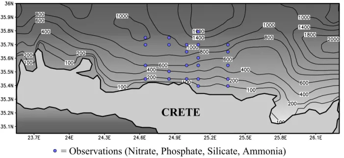
The modeled area is plotted in Fig. 2, extending from 23.575◦E to 26.3◦E and 35.075◦N to 36◦N. A horizontal resolution of 6 minutes was chosen, thus producing 56×20
= Observations (Nitrate, Phosphate, Silicate, Ammonia)
Fig. 2. Simulation domain with locations for profiles (pseudo) observations of nitrate, phosphate, silicate and ammonia.elements. In an attempt to account for the increased veloc-ity gradients near the surface, a logarithmic vertical distribu-tion was used with a total of 30 layers. The model was ini-tialized with climatological objectively analyzed temperature and salinity profiles from the Mediterranean Ocean Database (MODB-MED4), with a resolution of 1/4◦×1/4◦ for each MODB layer. Additionally, all initial velocities were set to zero. Wind stress fields derived from the ECMWF 1979– 1993 6-h reanalysis data and climatological heat flux fields of Bignami et al. (1995) were used for atmospheric forcing, while all biological variables were initialized from the 3-D ecological model for the Cretan Sea (Petihakis et al., 2002).
3 The SEPLEK filter
The estimation of long-range correlations associated with re-mote observations is a well-known difficulty of Kalman fil-tering methods (Bennett, 1992; Houtekamer and Mitchell, 1998). To tackle this problem, Houtekamer and Mitchell (1998) simply used a cutoff radius to exclude the effects of observations far away from the analysis location. However, the introduction of an “artificial” radius may be inconsistent with the correlations present in the estimation error covari-ance matrix, and might lead to numerical noise. Recently, a new framework to deal with this problem has been un-der development. It essentially involves the decomposition of the model domain into several sub-domains and the ap-plication of Kalman’s correction independently in each sub-domain, using an associated estimation covariance matrix (Anderson, 2003). Additional simplifications were also in-troduced to further reduce the computational burden using coarser grids (Fukumori, 2002) or EOFs (Testut et al., 2003; Ott et al., 2004), within the context of reduced-order and en-semble techniques, respectively. With the same aim in view,
Hoteit et al. (2001) introduced the SEPLEK filter to improve the local behavior of the SEEK filter and to reduce its com-putational cost. The main idea behind this filter is to force the correction directions of the SEEK filter to be local, by having as a support a small region of the domain, using a so-called “local EOF analysis”. To improve the representa-tion of the long-range variability, the local funcrepresenta-tions were complemented by global (classical) EOFs, leading to a set of “global-local” correction directions. The global functions can further be allowed to evolve with the model dynamics, as in the SEEK filter. The local functions remain invariant in order to retain their locality. This drastically reduces the computational burden with respect to the SEEK filter, since the number of global functions in practice can be small. It is important to note that, although the idea of the SEPLEK filter is similar to the filters cited above, its principle is different. The correction step of the Kalman filter actually remains un-changed in the SEPLEK filter and it is always applied glob-ally, while making use of global and local correction func-tions.
3.1 The global-local correction directions
To improve the representation of short-range correlations, a so-called “local EOF analysis” was introduced by Hoteit et al. (2001). The basic idea is to construct a set of EOFs, each having as a support a small region of the model domain. This is done by applying separate EOF analysis on a set of model sub-domains. To obtain adequate representation, these sub-domains should overlap. One efficient way to do this is to consider a partition of unity of the model domain, i.e. a set of positive functions {χ(j ), j =1, . . ., J } defined over the model domain whose sum is identically equal to 1. The model state vector X can then be decomposed into local fields X(j ), such as X=PJ
independent (classical) EOF analysis is then performed on each set of local fields X(j )to determine a representational
subspace for each sub-domain. The “global” representational error of the original state vector X can still be reduced by considering its projection onto the subspace spanned by the set of (local) EOFs of all the sub-domains.
Since the use of local functions only, may degrade the rep-resentation of the long-range variability, Hoteit et al. (2001), proposed to augment the local EOFs with some global func-tions. This would provide a set of functions suitable for the representation of the global, as well as the local model vari-ability. Such a set of “global-local” functions is obtained by performing a local EOF analysis on the residuals of the vec-tors X1, . . ., XN in the first global EOFs. This is supported
by the fact that these residuals are generally due to the bad representation of the local variability in the subspace spanned by the global EOFs. Recently, a similar idea was tested by Waseda et al. (2003), but using wavelets to represent the local fine-scale information.
3.2 Filter’s initialization
The global-local analysis does not readily provide a low-rank approximation of the error covariance matrix needed for the initialization of the filter. Therefore, we resort to an objective analysis to correct the initial state estimate ¯Xusing the initial observations Y0. In most applications, ¯Xis assumed to be the
average of a set of state vectors (provided by a historical run).
Starting from a set of global-local EOFs LB0=[L0...B], with rg
global EOFs (L0) and rl local EOFs (B), we take as initial
analysis state (Hoteit et al., 2001)
Xa(t0) = ¯X + LB0U0(LB0)THT0R −1 0 (Y o 0 −H0X),¯ (1) where U0=[(LB0)THT0R −1 0 H0LB0] −1, R
0is the initial
obser-vational error covariance matrix, and H0is the gradient of H0 evaluated at ¯X. This provides an initial analysis error
covariance matrix of rank (rg+rl),
Pa(t0) = LB0U0(LB0)T. (2)
3.3 Filter’s algorithm
As the Kalman filter, the SEPLEK filter provides an estimate of the system state as a succession of forecast and correction steps. Consider a physical system
Xt(tk) = M(tk−1, tk)Xt(tk−1) + ηk, (3)
where Xt(t )is the true state vector at time t, M(s, t ) is an
operator describing the system transition from time s to time
t, and ηk represents the model error. The forecast Xf(tk)is
obtained by integrating the model forward in time, starting from the most recent analyzed state Xa(tk−1). When a new
observation Ykois made, it is assumed to be a function of Xt and a measurement of uncertainty
Yko=HkXt(tk) + εk, (4)
where Hkis the observational operator and εk represents the
error in the observations. ηk and εk are assumed to be
in-dependent and normally distributed with zero mean and co-variance matrix Qk and Rk, respectively. Assuming that a
set of global-local correction directions LBk is available, the SEPLEK filter provides the analysis state, while using the observations sequentially to correct the forecast along the di-rections of LBk only, hence it will be called the “correction basis” of the filter, exactly as in the SEEK filter (Pham et al., 1998), Xa(tk) = Xf(tk) + LBkUk(LBk)THTkR −1 k [Y o k −HkX f(t k)], (5)
where Hkis the gradient of Hkevaluated at Xf(tk)and Ukis
updated with Uk−1=hUk−1+PLTB k QkPLB k i−1 +(LBk)THTkRk−1HkLBk. (6)
In the above equation, PLB k=[(L B k) TLB k] −1(LB k)is the
pro-jection operator onto the subspace generated by LBk. The corresponding analysis error covariance matrix is then given by
Pa(tk) = LBkUk(LBk)T. (7)
To attenuate the bad impact of different approximations and uncertainties on the performance of the filter, a forgetting factor ρ is used here. This factor enhances the filter stability by amplifying the already existing modes of the background error. It simply amounts to replacing Eq. (6) by
Uk−1=h1/ρUk−1+PLTB k QkPLB k i−1 +(LBk)THTkRk−1HkLBk. (8)
3.4 Evolution of the correction directions
The evolution of the correction directions is generally bene-ficial since it allows the filter to keep track of changes in the model dynamics (Hoteit et al., 2002). When a set of global-local functions is used as a correction basis for the filter, only the global functions can be allowed to evolve with the model dynamics, as in the SEEK filter, since the local EOFs would lose their local character. Although this significantly reduces the computational burden of the method, the “non-evolutive” nature of the local functions is clearly a disadvantage within the framework of the SEEK filter. This approximation, how-ever, is not expected to place a major limitation on the fil-ter’s performance, since the evolution equation of the SEEK filter is designed to follow only slow changes (Pham et al., 1998). This helps to support the idea of keeping the local functions invariant, since their evolution might be sometimes problematic as they represent quickly evolving local varia-tions by design. This means that we aim at not correcting all fine-scale variation errors, but only a large number of them, on average. If the correction basis is already decomposed as
LBk−1=[Lk−1... B]at time tk−1, we therefore take
Table 1. Twin experiments setup.
Assimilation Scheme SFEK, SFPLEK, SEPLEK State vector Ecosystem state variables Dimension of state vector 1 768 536
EOF analysis ≈3 years (360 vectors) Assimilation Period 5 March-5 June (3 months) Observed Variables Sea color or Profiles of
Nitrate, Phosphate, Silicate, Ammonia
Number of Observations Sea color: 693
Profiles: 23 stations ×30 layers =690
Assimilation time step 4 days Observation Error Sea color: 10%
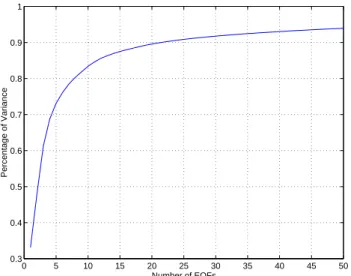
Profiles: 5% 0 5 10 15 20 25 30 35 40 45 50 0.3 0.4 0.5 0.6 0.7 0.8 0.9 1 Percentage of Variance Number of EOFs
Fig. 3. Percentage of variance explained by the EOFs versus the
number of retained EOFs.
where the new global correction directions Lk evolve with
the tangent linear model M (evaluated at Xf), as in the SEEK filter,
Lk =M(tk−1, tk)Lk−1. (10)
The forecast error covariance matrix can be then approxi-mated by
Pf(tk) = LBkUk−1(LBk)T +Qk. (11)
The structure of the forecast and analysis error covariance matrices of this filter is, therefore, very similar to that of the SEEK filter. Basically, these matrices are taken to be singular of low rank (or at least approximated to be so).
4 Experimental setup
The setup of the assimilation experiments is presented in this section. A general overview is given in Table 1.
4.1 The state vector
The variables of the physical sub-model, which are only used as forcing fields to the ecology, were considered perfect, and were therefore not included in the estimation process. This eliminates the influence of the forcing on the assimilation system performance, allowing to better understand the filter’s behavior with the ecological variables. The filter’s state vec-tor contains, therefore, the 88 state variables of the ecological model only. In more realistic applications, the assumption of perfect physics can be overoptimistic and the joint esti-mation of physical/biological variables may be necessary for a complete control of the coupled physical-ecological sys-tem. It should be noted that some biogeochemical variables may become negative after the filter’s correction. Following Natvik and Evensen (2003), these variables were simply set to a small threshold value close to zero, allowing species to become active again.
As mentioned above, the numerical grid of the Cretan Sea has 56 boxes in the zonal direction and 20 boxes in the merid-ional direction with 30 vertical layers. The corresponding water points for this grid are 20097, which multiplied by the 88 state variables of the ecological model, define the dimen-sion of the state vector to be equal to 1 768 536.
4.2 Choice of the filter’s correction directions
Global and local functions were determined using the classi-cal and loclassi-cal EOF analysis as described in Sect. 3.1. Follow-ing Pham et al. (1998), the EOF analysis was carried out on a set of state vectors simulated by the model itself. There-fore, the model was first integrated for 20 years with the aim of reaching a statistically steady state. Another integration of two more years was next carried out to generate a histor-ical sequence of model realizations. A sequence HSof 360
state vectors was retained by storing one state vector every two days. As the ecological state variables are of a differ-ent nature, each variable was normalized by the inverse of its spatially-averaged (over all the grid points) standard devi-ation. Figure 3 plots the cumulative percentage of variance explained by the EOFs as a function of the number of EOFs. As expected, the first EOFs capture most of the variability of the system, while the last EOFs are reduced to noise. For instance, the first 20 EOFs explain 90% of the observed vari-ability in the sample HS.
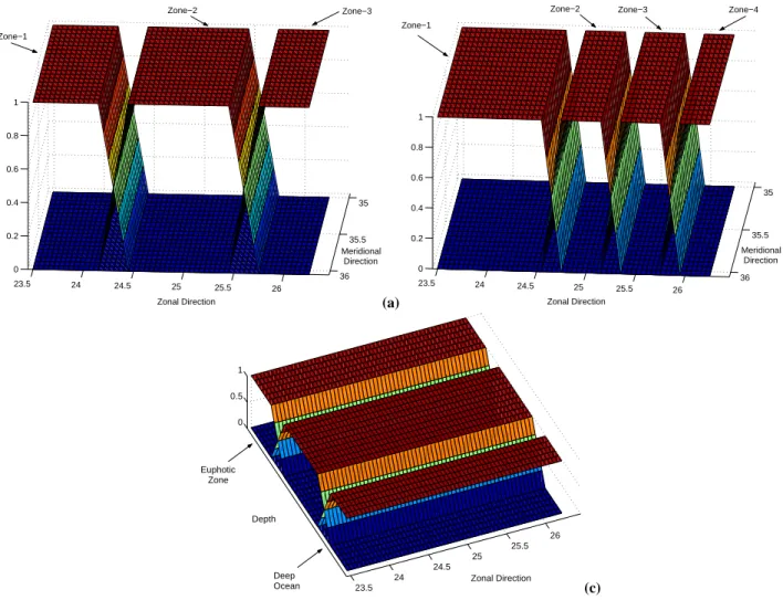
Different sets of local EOFs were determined by decom-posing the model domain into horizontal and vertical sub-domains, according to the spatial variability of the Cretan Sea ecosystem. The local analysis was performed on the residuals of the states in the first 3, 6 and 9 global EOFs, which explain 63%, 72% and 80% of the total variance of the sample HS, respectively. In the horizontal direction, the
35 35.5 36 23.5 24 24.5 25 25.5 26 0 0.2 0.4 0.6 0.8 1 Meridional Direction Zonal Direction Zone−1 Zone−2 Zone−3 (a) 35 35.5 36 23.5 24 24.5 25 25.5 26 0 0.2 0.4 0.6 0.8 1 Meridional Direction Zonal Direction Zone−1
Zone−2 Zone−3 Zone−4
(b) 23.5 24 24.5 25 25.5 26 0 0.5 1 Zonal Direction Depth Euphotic Zone Deep Ocean (c)
Fig. 4. Model domain decomposition into 3 and 4 horizontal sub-domains and 3 vertical sub-domains.
model domain was decomposed into three and four overlap-ping sub-domains, using the partitions of unity functions as shown in Fig. 4. In both cases, the width of the overlapping areas was set to 1/6◦. The first decomposition was used when profile data are assimilated to isolate the observed area, as il-lustrated in Fig. 2, limiting in this way the range of the filter’s corrections to this area only. The second decomposition was applied to isolate the different observed spatial variabilities in the model. Separate EOF analysis were then applied on the projections of the state vectors of the sample HSon each
of these sub-domains. Another decomposition in the vertical direction was also carried out, according to the natural ver-tical variability that the ecosystem could exhibit: euphotic zone, deep-ocean, and the area in between. The depth of the euphotic sub-domain was set to the first 200 m, with an overlapping zone of 50 meters between the two sub-domains. The deep ocean was also decomposed into two sub-domains (Fig. 4). Obviously, the local EOFs of the deep ocean zones do not produce any corrections when surface ocean color data are assimilated. The use of global functions may, therefore, be crucial in this case for an efficient propagation of surface information to the deep ocean.
4.3 Data and filter validation - twin experiments
A twin experiments approach was adopted for this study, in which the “truth” is assumed to be provided by the model itself. Therefore, a set of 45 reference (true) states (Xt) is first retained from a reference model free-run, sampled ev-ery two days from March to June. This period is marked by the increased primary production of the system, and it has been chosen in order to test the effectiveness of the fil-ters during strongly variable periods. Pseudo-observations for the assimilation experiments are then extracted from the
Xt. These states are also later used to evaluate the filter’s performance by comparing them with the fields produced by the assimilation system. The multivariate properties of the filters can, therefore, be assessed by examining the impact of the assimilation system on non-observed variables. Pseudo-observations of ocean color data were sampled from the ref-erence states Xt over the entire surface domain. Pseudo-profiles data of nitrate, phosphate, silicate and ammonia were sampled following a realistic network of 23 stations in the Cretan Sea (Fig. 2). Random Gaussian noises with zero mean and standard deviation of 5% for the profiles and 10% for the
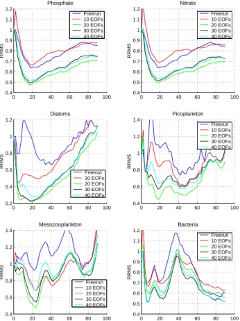
0 20 40 60 80 100 0.4 0.6 0.8 1 1.2 1.4 Mesozooplankton RRMS Freerun 10 EOFs 20 EOFs 30 EOFs 40 EOFs 0 20 40 60 80 100 0.4 0.5 0.6 0.7 0.8 0.9 1 1.1 1.2 Bacteria RRMS Freerun 10 EOFs 20 EOFs 30 EOFs 40 EOFs 0 20 40 60 80 100 0.4 0.5 0.6 0.7 0.8 0.9 1 1.1 1.2 Phosphate RRMS Freerun 10 EOFs 20 EOFs 30 EOFs 40 EOFs 0 20 40 60 80 100 0.4 0.5 0.6 0.7 0.8 0.9 1 1.1 1.2 Nitrate RRMS Freerun 10 EOFs 20 EOFs 30 EOFs 40 EOFs 0 20 40 60 80 100 0.2 0.4 0.6 0.8 1 1.2 Diatoms RRMS Freerun 10 EOFs 20 EOFs 30 EOFs 40 EOFs 0 20 40 60 80 100 0.4 0.6 0.8 1 1.2 1.4 Picoplankton RRMS Freerun 10 EOFs 20 EOFs 30 EOFs 40 EOFs
Fig. 5. Evolution in time of phosphate, nitrate, diatoms,
picoplank-ton, mesozooplankton and bacteria RRMS from the model free-run and the SFEK filter assimilating profiles with 10, 20, 30 and 40 EOFs.
ocean color were also added to the pseudo-observations in order to construct a more realistic framework. In all the as-similation experiments, the initial state of the filter is chosen to be the mean state of the sample HS.
The performance of the filters is assessed through the rel-ative root mean square (RRMS) error over the whole model domain for each state variable. The RRMS is defined as
RRMS(tk) =
kXt(tk) − Xa(tk)k
kXt(t
k) − ¯Xk
, (12)
where Xais the analysis state obtained by the filter, ¯Xis the mean state of the sample HS and k·k denotes the Euclidean
norm. The error is therefore relative to the free-run error, since the denominator represents the error when no observa-tions are assimilated and the analysis vector is taken as the mean state of the historical free-run.
5 Assimilation results
Several experiments were carried out to evaluate the repre-sentativeness of the different set of global-local EOFs and to assess the relevance of the assimilation system. The choice of the domain decomposition to make best use of the available
observations was carefully assessed. As stated before, all sensitivity experiments were performed using the SFPLEK filter since it provides an efficient low-cost way to evaluate the representativeness of the different global-local EOFs. Al-though the assimilation results will not be identical as if the SEPLEK filter was used, we expect the sensitivities of both filters to the different correction directions to be very similar. The experimental results are focused on those variables con-sidered as important in revealing the dynamics of the ecosys-tem (nutrients, phytoplankton and bacteria), and are those parameters most often measured in sampling programs.
The forgetting factor ρ is used to artificially stimulate the filter’s forecast covariance matrix as a simple way to com-pensate for the different approximations used in the filter, as the use of low-rank covariance matrices and the linearization of the system equations. Its value is therefore a priori un-known, since it completely depends on the characteristics of the assimilation scheme and the system under study. Here we resort to experimentation to find an appropriate value for
ρ. Several assimilation runs (not shown here) were therefore first performed with the SFPLEK filter, to study the behavior of the assimilation system with different values of ρ vary-ing between 0.5 and 1. The best results were obtained usvary-ing
ρ=0.9, which was therefore used in all the experiments pre-sented below.
5.1 Assimilation of profiles of data
The assimilation results of data profiles are first presented. The assimilation results of sea color data are discussed in the next section.
5.1.1 Sensitivity to the number of global EOFs
The first experiment was performed with the SFEK filter us-ing global (classical) EOFs only. The goal was to show that the performance of the filter stagnates (even degrades in cer-tain situations), when the number of global EOFs increases. The SFEK filter was therefore implemented with 10, 20, 30 and 40 EOFs. The performance of the filter was also com-pared to the model free-run (without assimilation) to assess the relevance of the assimilation system. The RRMS of these runs are illustrated in Fig. 5. The assimilation system en-hances the model behavior in all cases. For most of the vari-ables, the filter performs best with 20 EOFs. This suggests that the last global EOFs do not represent any specific mode of the system and are very often reduced to noise. Only bac-teria seems to require more than 20 EOFs, but this is proba-bly due to the short-range variations of this variable. Overall, the SFEK filter with global EOFs fails to stabilize the RRMS completely, particularly for diatoms and mesozooplankton. Assimilation results for diatoms needs to be improved and can be explained by the significant spatial and temporal vari-ations during the winter mixing. As nutrients are transported in the euphotic zone, the conditions become particularly fa-vorable for big cells as diatoms, significantly increasing their contribution to the overall primary production. This local
behavior is generally difficult to capture by the global (clas-sical) EOFs. Although mesozooplankton grows at a slower rate compared to diatoms, the latter phytoplanktonic group accounts for a significant proportion of the mesozooplank-ton’s diet, thus explaining a part of the variability.
5.1.2 Sensitivity to the choice of the correction directions
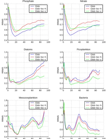
The performance of the SFEK/SFPLEK filter strongly de-pends on the representativeness of its invariant correction ba-sis (Hoteit et al., 2002), therefore, providing a very efficient way to measure the relevance of the different set of global-local EOFs. Figure 6 compares the results of three exper-iments using 20 correction directions as follows: (i) global (classical) EOFs, 6 global and 14 local of EOFs (in each sub-domain) from (ii) the horizontal and (iii) the vertical decom-position into three sub-domains, as described in Sect. 4.2. With the exception of phosphate and nitrate, one can see that the use of local EOFs clearly enhances the filter’s behavior. This is consistent with the results of Hoteit et al. (2001) who found that the use of local EOFs only, may badly affect the estimation of the model variables governed by long-range circulations, such as phosphate and nitrate. The overall im-provements to the fine-scale variability are still however not quite significant. We speculate that the limited impact of this choice of domain decomposition on the filter’s performance is probably due to a weak spatial variability in the small do-main of the model, allowing good representation of the hor-izontal correlations by the classical EOFs. Concerning the vertical decomposition, the separation of the euphotic zone from the deep ocean clearly improves the assimilation re-sults. It greatly enhances the estimation of those variables with strong variability in the euphotic zone. The use of ver-tical EOFs seems to provide a remarkably efficient repre-sentation of the different local variabilities in the ecosystem model. For instance, the estimation of mesozooplankton fol-lows diatoms with small error in the first 25 days of assim-ilation. However as spring progresses and other functional groups increase also, mesozooplankton decreases the propor-tion of diatoms in its diet. This, in conjuncpropor-tion with the high excretion rate of uptake, contributes to a strong variability and explains part of the increase in the estimation error.
5.1.3 Sensitivity to the number of global EOFs in the global-local functions
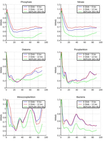
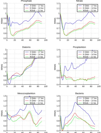
The aim of this experiment is to study the sensitivity of the filter to the number of global EOFs in the global-local cor-rection basis. Once this number is fixed, the number of local EOFs to be retained in each sub-domain can then be chosen, according to the percentage of variance explained by these EOFs (as it is usually done in the classical EOFs). Two runs were performed with the SFPLEK filter, using global-local EOFs obtained from the vertical decomposition, always with 20 correction directions: (i) 6 global and 14 local, and (ii) 3 global and 17 local, respectively. The RRMS for these runs are plotted in Fig. 7. It can be seen that the use of more global
0 20 40 60 80 100 0.4 0.6 0.8 1 1.2 1.4 1.6 1.8 Mesozooplankton RRMS Glob Glob−loc−h Glob−loc−z 0 20 40 60 80 100 0.4 0.6 0.8 1 1.2 1.4 Bacteria RRMS Glob Glob−loc−h Glob−loc−z 0 20 40 60 80 100 0.4 0.5 0.6 0.7 0.8 0.9 1 1.1 Phosphate RRMS Glob Glob−loc−h Glob−loc−z 0 20 40 60 80 100 0.4 0.5 0.6 0.7 0.8 0.9 1 1.1 Nitrate RRMS Glob Glob−loc−h Glob−loc−z 0 20 40 60 80 100 0 0.2 0.4 0.6 0.8 1 1.2 1.4 Diatoms RRMS Glob Glob−loc−h Glob−loc−z 0 20 40 60 80 100 0.2 0.4 0.6 0.8 1 1.2 1.4 1.6 Picoplankton RRMS Glob Glob−loc−h Glob−loc−z
Fig. 6. Evolution in time of phosphate, nitrate, diatoms,
picoplank-ton, mesozooplankton and bacteria RRMS from the SFEK/SFPLEK filter assimilating profiles using global EOFs (SFEK filter), global-local EOFs (SFPLEK filter), from 3 horizontal and 3 vertical sub-domains (as shown in Fig 4).
EOFs enhances the assimilation results for phosphate and ni-trate. However, mesozooplankton seems to be better esti-mated with less global EOFs. This might be expected since nitrate and phosphate variables have a long-range variability while mesozooplankton is mostly dominated by small-scale variations. Changing the number of global EOFs has almost no effect on picoplankton and bacteria. The number of global EOFs should therefore be chosen very carefully while bal-ancing between the estimation quality of the different vari-ables of the model. Its choice depends only on the system under study and the variables that need to be estimated with more precision.
5.1.4 Sensitivity to the choice of the horizontal sub-domains
The last sensitivity experiment was carried out to study the performance of the assimilation system with respect to the choice of the horizontal sub-domains. More precisely, the SFPLEK filter was tested with two different sets of global-local EOFs which have been computed from the two de-compositions of the model domain into 3 and 4 horizon-tal sub-domains, as described in Sect. 4.2. One can see
0 20 40 60 80 100 0.4 0.5 0.6 0.7 0.8 0.9 1 1.1 1.2 Mesozooplankton RRMS 6 Glob − 9 loc 3 Glob − 12 loc SEPLEK (6G+9L) 0 20 40 60 80 100 0.2 0.4 0.6 0.8 1 1.2 Bacteria RRMS 6 Glob − 9 loc 3 Glob − 12 loc SEPLEK (6G+9L) 0 20 40 60 80 100 0.4 0.5 0.6 0.7 0.8 0.9 1 1.1 1.2 Phosphate RRMS 6 Glob − 9 loc 3 Glob − 12 loc SEPLEK (6G+9L) 0 20 40 60 80 100 0.4 0.5 0.6 0.7 0.8 0.9 1 1.1 1.2 Nitrate RRMS 6 Glob − 9 loc 3 Glob − 12 loc SEPLEK (6G+9L) 0 20 40 60 80 100 0 0.2 0.4 0.6 0.8 1 Diatoms RRMS 6 Glob − 9 loc 3 Glob − 12 loc SEPLEK (6G+9L) 0 20 40 60 80 100 0.2 0.4 0.6 0.8 1 1.2 Picoplankton RRMS 6 Glob − 9 loc 3 Glob − 12 loc SEPLEK (6G+9L)
Fig. 7. Evolution in time of phosphate, nitrate, diatoms,
picoplank-ton, mesozooplankton and bacteria RRMS from the SFPLEK filter assimilating profiles using global-local EOFs from 3 vertical sub-domains with 3 global − 17 local EOFs, 6 global −14 local EOFs, and from the SEPLEK filter with 6 global - 14 local EOFs.
from the results of these runs plotted in Fig. 8 that the fil-ter’s performance highly depends on the choice of the sub-domains. Moreover, increasing the number of sub-domains does not necessarily improve the assimilation results. Sur-prisingly, only the estimation of the picoplankton was better when more sub-domains were used. In general, limiting the length of the corrections in the horizontal direction seems to enhance the filter performance by filtering noises caused by poorly known correlations in the covariance matrix. How-ever, the choice of the decomposition must also take into ac-count the different local variabilities of the model, as well as the type of assimilated observations.
5.1.5 Evolution of the global correction directions - SE-PLEK filter
The evolution of the correction directions is important for keeping track of changes in the model dynamics. As stated in Sect. 3.4, when a set of global-local functions is used, only the global functions can be allowed to evolve in time to fol-low changes in the model dynamics. In this experiment, a set of 6 global and 9 vertical local EOFs (in each sub-domain) were used in the SFPLEK and the SEPLEK filters. The only
0 20 40 60 80 100 0.4 0.5 0.6 0.7 0.8 0.9 1 1.1 1.2 Mesozooplankton RRMS 3 zones 4 zones 0 20 40 60 80 100 0.4 0.5 0.6 0.7 0.8 0.9 1 1.1 1.2 Bacteria RRMS 3 zones 4 zones 0 20 40 60 80 100 0.4 0.5 0.6 0.7 0.8 0.9 1 1.1 1.2 Phosphate RRMS 3 zones 4 zones 0 20 40 60 80 100 0.4 0.5 0.6 0.7 0.8 0.9 1 1.1 1.2 Nitrate RRMS 3 zones 4 zones 0 20 40 60 80 100 0.2 0.4 0.6 0.8 1 1.2 Diatoms RRMS 3 zones 4 zones 0 20 40 60 80 100 0.4 0.5 0.6 0.7 0.8 0.9 1 1.1 1.2 Picoplankton RRMS 3 zones 4 zones
Fig. 8. Evolution in time of phosphate, nitrate, diatoms,
picoplank-ton, mesozooplankton and bacteria RRMS from the SFPLEK filter assimilating profiles using global-local EOFs from 3 and 4 horizon-tal and 4 sub-domains (as shown in Fig 4).
difference between the two runs was that the global direc-tions evolve in time in the SEPLEK filter, while they remain unchanged in the SFPLEK filter. The computational cost of the former was therefore six times higher than the latter. This is affordable with the current computers, and is noticeably faster than the SEEK filter, which usually requires the evolu-tion of more than 30 funcevolu-tions for the studied ecosystem.
The higher cost of the SEPLEK filter can be supported by Fig. 7, which plots the RRMS for the two runs. Indeed, one can clearly see that the evolution of the global directions en-hances the assimilation results for all the model variables. It also improves the stability of the filter due to the contin-uous tracking of the changes in the model dynamics. Only the RRMS for the mesozooplankton was not significantly im-proved. This points to difficulties in the SEEK update equa-tion of the correcequa-tion direcequa-tions to follow rapid changes in the model.
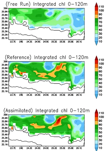
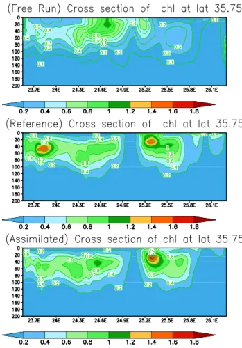
Integrated chlorophyll concentrations (0 m–120 m) of the assimilated, the reference, and the free-runs, for the May, are plotted in Fig. 9. The filter follows closely the pseudo-observations reproducing the spatial distribution, as well as the range of values. An interesting feature is the local low concentration area at the center - top part of the domain, at-tributed to the existence of an intense anticyclone (Petihakis
Fig. 9. Integrated chlorophyll concentrations (mg/m3) between 0 m–120 m from the free run, the reference run, as estimated by the SEPLEK filter.
et al., 2002; Triantafyllou et al., 2003b), transferring nutri-ents in the deeper layers. The action of another anticyclone is also observed at the east part of the simulation field, as is also evident by the low concentration values. Between these two gyres the intrusion of nutrients in the euphotic zone is depicted by maximum concentrations of chlorophyll. The areas with low chlorophyll concentrations, caused by the gy-ral system of the two anticyclones, is also nicely simulated by the free run. The later, however, fails to reproduce the in-creased chlorophyll concentrations close to the coast and be-tween the two anticyclones. For the same period integrated bacterial biomass also exhibits a very good coincidence be-tween the two runs (Fig. 10). The importance of the physical features in the ecosystem functioning is evident, with bac-terial biomass following the distribution of chlorophyll, al-though maximum values are developed closer to the coast. This is because the spring bloom which started in the coastal areas in late winter, provides the important food substrate for bacterial growth. Additionally, a cross section of chlorophyll concentrations of the three runs (with assimilation, reference, free) along the east–west direction, at latitude 35.75◦N, is illustrated in Fig. 11. The simulations are very similar,
pro-Fig. 10. Integrated bacterial biomass between 0 m–120 m from the
free run, the reference run, as estimated by the SEPLEK filter.
ducing a characteristic feature of the Cretan Sea ecosystem, a Deep Chlorophyll Maximum (DCM), which as the ther-mocline formation progresses (August), reaches as deep as 90–100 m. The presence of the anticyclone at the center of the domain is nicely depicted by the low chlorophyll concen-trations.
5.2 Assimilation of ocean color data
Assimilation experiments of ocean color data are presented in this section. The aim of these runs is to show that the choice of the domain’s decomposition should take into ac-count the characteristics of the observations to be assimilated into the model. Several sensitivity experiments using the SF-PLEK filter were performed, as in the later section. Here only the assimilation results of two assimilation experiments are discussed. The first experiment deals with the sensitivity to the choice of the domain decomposition, while the sec-ond assesses the impact of the number of global EOFs in the vertical global-local functions on the filter’s behavior.
For the first experiment, three runs were carried out as in Sect. 5.1.1: (i) 20 global (classical) EOFS, (ii) 6 global and 14 local EOFs for the horizontal decomposition into 4 sub-domains (which provided better results in our experiments than the horizontal decomposition into 3 sub-domains), and
Fig. 11. Vertical cross sections of chlorophyll concentrations (mg/m3) at latitude 35.75◦E from the free run, the reference run, as estimated by the SEPLEK filter.
(iii) 9 global and 11 local EOFs from the decomposition into vertical sub-domains. The RRMS for these runs are pre-sented in Fig. 12. At first glance, the assimilation of sea color data significantly improves the estimation of picoplankton, mesozooplankton and bacteria compared to the experiment of assimilating data profiles. Phosphate and nitrate are well estimated by the filter, noting that these data have very little effect on diatoms. Although in the beginning of the exper-imental period diatoms are dependent on the availability of phosphate and nitrate (small error), soon after they are lim-ited by silicate, while a significant pressure is also exerted by predators. Additionally, the assimilation of sea color data affects chlorophyll concentrations only at the top layer of the euphotic zone and thus it provides relatively less information about diatoms, which are mostly concentrated at deep layers because of their heavy weight. The use of global-local cor-rection dicor-rections generally enhances the filter’s behavior for all variables, although the improvements are not significant. In contrast to the assimilation of data profiles, the horizontal decomposition seems to provide better results, while the im-pact of the vertical decomposition is less pronounced. In par-ticular, phosphate and nitrate are better assimilated when hor-izontal local EOFs are used, probably because of the global
0 20 40 60 80 100 0.2 0.4 0.6 0.8 1 1.2 1.4 1.6 Mesozooplankton RRMS Free−run Glob Glob−loc−h Glob−loc−z 0 20 40 60 80 100 0.2 0.4 0.6 0.8 1 1.2 Bacteria RRMS Free−run Glob Glob−loc−h Glob−loc−z 0 20 40 60 80 100 0.4 0.6 0.8 1 1.2 1.4 Phosphate RRMS Free−run Glob Glob−loc−h Glob−loc−z 0 20 40 60 80 100 0.4 0.6 0.8 1 1.2 1.4 Nitrate RRMS Free−run Glob Glob−loc−h Glob−loc−z 0 20 40 60 80 100 0.5 1 1.5 2 Diatoms RRMS Free−run Glob Glob−loc−h Glob−loc−z 0 20 40 60 80 100 0.2 0.4 0.6 0.8 1 1.2 1.4 1.6 Picoplankton RRMS Free−run Glob Glob−loc−h Glob−loc−z
Fig. 12. Evolution in time of phosphate, nitrate, diatoms,
picoplank-ton, mesozooplankton and bacteria RRMS from the SFPLEK filter assimilating sea color data using global EOFs, global-local EOFs from 4 horizontal and 3 vertical sub-domains (as shown in Fig 4).
coverage of color data to all sub-domains. Limiting the prop-agation of the surface data by using vertical local EOF, de-grades the filter’s performance for these two variables and as one can expect, the classical global EOFs still provide the best estimations.
In an attempt to explain why the vertical decomposition is not as efficient as in the assimilation of profiles data, three assimilation runs were performed using vertical global-local correction functions with: (i) 3 global and 17 local, (ii) 6 global and 14 local, and (iii) 9 global and 11 local. Figure 13 depicts the RRMS under the euphotic zone for the three runs. As can be seen, the use of more global EOFs, up to a certain number, improves the filter’s performance in the deep ocean. This suggests that an appreciable number of global EOFs are still needed to propagate the surface data into the deep layers. This was not always true (not presented here) for all model variables in the euphotic zone, and the use of local EOFs gen-erally improves the assimilation results. These results are not in full agreement with those of Carmillet et al. (2001), who found that the use of only local EOFs in the euphotic zone improves the filter’s behavior. We speculate that this is prob-ably due to a weak representation of the surface/subsurface correlations in their (global) EOFs. The results of this exper-iment, however, confirm the Carmillet et al. (2001) finding,
namely that the existence of “bad correlations” in the correc-tion direccorrec-tions has a more severe impact on the vertical than on the horizontal direction.
In another experiment similar to the one performed in Sect. 5.1.5, but assimilating ocean color data, the SEPLEK filter was used to assess the relevance of the evolution of the global correction directions. The results of this run were consistent with Sect. 5.1.5 and lead to identical conclusions. Therefore, we decided not to show them in order to save space.
6 Summary and discussion
While data assimilation techniques have made great progress in meteorology and physical oceanography, their application to complex ecosystem models often encounters many diffi-culties, mainly because of the huge number of ecological variables and of their complex variabilities. In this paper, sophisticated Kalman filters, called SFPLEK and SEPLEK, were used to assimilate profiles and sea color data into a 3-D coupled biophysical model of the Cretan Sea ecosystem. These filters make use of a combination of global (classical) and so-called local EOFs to supplement the large-scale vari-ability continued by the classical EOFs with local fine-scale information. The local EOFs are determined according to the different variability of the ecosystem model, as well as to the characteristics of the assimilated observation. Moreover, the global EOFs can be allowed to evolve with the model dy-namics, and this was found to be beneficial for the stability of the filter during periods of strong ecological variability.
From the various twin experiments performed, the perfor-mances of the SFPLEK and SEPLEK filters were satisfactory for assimilating sea color data and profiles of nitrate, phos-phate, silicate and ammonia from 23 stations in the Cretan Sea, without requiring large computational resources. The assimilation results also suggest that the use of local func-tions, obtained from a horizontal or a vertical domain decom-position, clearly improves the representativeness of the fil-ter’s correction basis. Sensitivity experiments also revealed that an efficient choice of horizontal decomposition should take into account both the different local variabilities of the system and the distribution of the data. A horizontal decom-position was found, however, to have less of an impact than a vertical decomposition, probably because of the small area of the computational field which make the classical EOFs less noisy in the horizontal direction. The assimilation ex-periments also confirm previous results by stating that the ecosystem models are more sensitive to bad correlations in the vertical than in the horizontal direction. The use of lo-cal vertilo-cal EOFs was found to be beneficial for enhancing the stability of the filter, as long as they are complemented with a number of global EOFs for an efficient representation of the model large-scale variability. This was more evident when sea color data were assimilated to help propagating sur-face information into the deep layers. More experiments with different vertical decompositions still need to be carried out
0 20 40 60 80 100 0.2 0.4 0.6 0.8 1 1.2 1.4 1.6 Mesozooplankton RRMS 3 Glob − 17 loc 6 Glob − 14 loc 9Glob − 11 loc 0 20 40 60 80 100 0.4 0.6 0.8 1 1.2 1.4 1.6 1.8 Bacteria RRMS 3 Glob − 17 loc 6 Glob − 14 loc 9Glob − 11 loc 0 20 40 60 80 100 0.5 0.6 0.7 0.8 0.9 1 1.1 1.2 Phosphate RRMS 3 Glob − 17 loc 6 Glob − 14 loc 9Glob − 11 loc 0 20 40 60 80 100 0.5 0.6 0.7 0.8 0.9 1 1.1 1.2 Nitrate RRMS 3 Glob − 17 loc 6 Glob − 14 loc 9Glob − 11 loc 0 20 40 60 80 100 0.4 0.6 0.8 1 1.2 1.4 1.6 1.8 2 Diatoms RRMS 3 Glob − 17 loc 6 Glob − 14 loc 9Glob − 11 loc 0 20 40 60 80 100 0.4 0.6 0.8 1 1.2 1.4 Picoplankton RRMS 3 Glob − 17 loc 6 Glob − 14 loc 9Glob − 11 loc
Fig. 13. Evolution in time of phosphate, nitrate, diatoms,
picoplank-ton, mesozooplankton and bacteria RRMS in the deep ocean from the SFPLEK filter assimilating sea color data using global-local EOFs from the vertical decomposition with: (i) 6 global - 14 lo-cal EOFs, and (ii) 9 global - 11 lolo-cal EOFs.
to tune the parameters of the vertical sub-domains. At this stage, however, we thought that it is more important to better understand the impact of different horizontal sub-domains, since the sensitivity of the filter to the latter is more unpre-dictable. Recently, the availability of ocean color data pro-vided a unique opportunity for the problem of data assimila-tion in ecosystem models due to their global coverage. How-ever, these data contain only information about the surface layers of the ocean, and therefore still need to be comple-mented with in-situ data of the lower layers, as suggested by the results of our experiments.
Twin experiments have demonstrated the ability of the SF-PLEK and SESF-PLEK filters to efficiently control the evolu-tion of the ecosystem state, while assimilating profiles and sea color data into a small area of the Cretan Sea during a period of strong ecosystem variability. As a next step, real profiles and ocean color data will be assimilated, which often proves to be much more complex and less forgiving than a twin experiments approach. This would point to the need for incorporating a more sophisticated model er-ror, since ecosystem models are only a crude approxima-tion of the real system under study. We also plan to test the filters using local functions obtained from simultaneous
horizontal-vertical decompositions. The preliminary twin experiment applications reported in this paper were, how-ever necessary, providing important knowledge and experi-ence, and enabling the assessment of the impact of the fil-ter on non-observed variables. An extension of the model configuration to cover the Eastern Mediterranean is a future task in the framework of the project Mediterranean Forecast-ing System Toward Environmental Predictions (MFSTEP) (http://www.bo.ingv.it/mfstep/), which might reveal a greater impact of a horizontal decomposition of the simulation do-main.
Acknowledgements. This work was carried out within the frame-work of the project Mediterranean Forecasting System Toward Environmental Predictions (MFSTEP). The authors would like to thank A. Eleftheriou for his constructive criticism during the prepa-ration of this work, and M. Eleftheriou for her help in editing this text.
Topical Editor N. Pinardi thanks two referees for their help in evaluating this paper.
References
Allen, J., Ekenes, M., and Evensen, G.: An Ensemble Kalman Fil-ter with a complex marine ecosystem model: Hindcasting phyto-plankton in the Cretan Sea, Ann. Geophys., 21, 399–411, 2003,
SRef-ID: 1432-0576/ag/2003-21-399.
Anderson, L.: A local least squares framework for ensemble filter-ing, Monthly Weather Review, 131, 634–642, 2003.
Baretta, J., Ebenhoh, W., and Ruardij, P.: The European Regional Seas Ecosystem Model, a complex marine ecosystem model, Netherlands Journal of Sea Research, 33, 233–246, 1995. Bennett, A.: Inverse methods in physical oceanography, Cambridge
Univ. Press, 346, 1992.
Bignami, F., Marullo, S., Santoleri, R., and Schiano, M. E.: Long-wave radiation budget in the Mediterranean Sea, J. Geophys. Res., 100, 2501–2514, 1995.
Blumberg, A. F. and Mellor, G. L.: A description of a three-dimensional coastal ocean circulation model, in: Three-Dimensional Coastal Ocean Circulation Models, edited by: N. Heaps, Coastal Estuarine Science, 1–16, AGU, Washington, D.C., 4th Ed., 1987.
Brasseur, P., Ballabrera-Poy J., and Verron J.: Assimilation of al-timetric observations in a primitive equation model of the Gulf stream using a singular evolutive extended Kalman filter, Journal of Marine Systems, 22(4), 269–294, 1999.
Burgers, G., Van Leeuwen, P., and Evensen, G.: Analysis scheme in the ensemble Kalman filter, Monthly Weather Review, 126, 1719–1724, 1998.
Cane, M., Kaplan, A., Miller, R., Tang, B., Hackert, E., and Busalacchi, A.: Mapping tropical Pacific sea level: data assim-ilation via a reduced state Kalman filter, J. Geophys. Res., 101, 22 599–22 617, 1995.
Carmillet, V., Brankart, J. M., Brasseur, P., Drange, H., Evensen, G., and Verron, J.: A singular evolutive extended Kalman filter to assimilate ocean color data in a coupled physical-biochemical model of the North Atlantic ocean, Ocean Modelling, 3, 167– 192, 2001.
Evans, G.: The role of local models and data sets in the Joint Ocean global Flux study, Deep Sea Research I, 46, 1369–1389, 1999.
Evensen, G. and van Leeuwen, P. J.: Assimilation of Geosat altime-ter data for the Agulhas current using the ensemble Kalman filaltime-ter with a quasi-geostrophic model, Monthly Weather Review, 124, 85–96, 1994.
Faugeras, B., Levy, M., Memery, L., Verron, J., Blum, J., and Charpentier, I.: Can biogeochemical fluxes be recovered from nitrate and chlorophyll data? A case study assimilating data in the Northwestern Mediterranean Sea at the JGOFS-DYFAMED station, Journal of Marine Systems, 40, 99–125, 2003.
Fukumori, I.: A partitioned Kalman filter and smoother. Monthly Weather Review, 130, 1370–1383, 2002.
Fukumori, I. and Malanotte-Rizzoli, P.: An approximate Kalman filter for ocean data assimilation: an example with an idealized Gulf Stream model, J. Geophys. Res., 100, 6777–6793, 1995. Harmon, R. and Challenor, P.: A Markov chain Monte Carlo
method for estimation assimilation into models, Ecological mod-elling, 101, 41–59, 1996.
Hoteit, I., Pham, D. T., and Blum, J.: A semi-evolutive partially local filter for data assimilation, Marine Pollution Bulletin, 43, 164–174, 2001.
Hoteit, I., Pham, D.-T., and Blum, J.: A simplified reduced-order kalman filtering and application to altimetric data assimilation in tropical pacific, Journal of Marine Systems, 36, 101–127, 2002. Hoteit, I., Triantafyllou, G., Petihakis, G., and Allen, J. I.: A
singu-lar evolutive extended Kalman filter to assimilate real in situ data in a 1-D marine ecosystem model, Ann. Geophys., 21, 389–397, 2003,
SRef-ID: 1432-0576/ag/2003-21-389.
Houtekamer, P. and Mitchell, H.: Data assimilation using an en-semble Kalman filter technique, Monthly Weather Review, 126, 796–811, 1998.
Lawson, L., Hofmann, E., and Spitz, Y.: Time series sampling and data assimilation in a simple marine ecosystem model, Deep Sea Research II, 43, 625–651, 1996.
Malanotte-Rizzoli, P.: Modern approaches to data assimilation in ocean modeling, Elsevier Oceanography Series, 61, Elseiver, P.O. Box 211, 1000 AE Amsterdam, The Netherlands, 455, 1996.
Matear, R. J.: Parameter optimization and analysis of ecosystem models using simulated annealing: A case study at station P, Journal of Marine Research, 53, 571–607, 1995.
Natvik, L. and Evensen, G.: Assimilation of ocean color data into a biochemical model of the North Atlantic. Part-I. Data assimi-lation experiments, Journal of Marine Systems, 40–41, 127–153, 2003.
Natvik, L., Eknes, M., and Evensen, G.: A weak constraint inverse for a zero-dimensional marine ecosystem model, Journal of Ma-rine Systems, 28, 19–44, 2001.
Ott, E., Hunt, B. R., Szunyogh, I., Zimin, A. V., Kostelich, E. J., Corazza, M., Kalnay, E., Patil, D. J., and Yorke, J. A.: A Lo-cal Ensemble Kalman Filter for Atmospheric Data Assimilation, Tellus, 56A, 415-428, 2004.
Petihakis, G., Triantafyllou, G., Allen, J., Hoteit, I., and Dounas, C.: Modelling the Spatial and Temporal Variability of the Cretan Sea Ecosystem, Journal of Marine Systems, 36, 173–196, 2002. Pham, D., Verron, J., and Roubaud, M.: Singular evolutive Kalman
filter with EOF initialization for data assimilation in oceanogra-phy, Journal of Marine Systems, 16, 323–340, 1998.
Testut, C., Brasseur, P., Brankart, J.-M., and Verron, J.: Assimila-tion of sea-surface temperature and altimetric observaAssimila-tions dur-ing 1992–1993 into an eddy permittdur-ing primitive equation model of the North Atlantic Ocean, Journal of Marine Systems, 40–41,
291–316, 2003.
Thingstad, T., Havskum, H., Kaas, H., Nielsen, T., Riemann, B., Lefevre, D., and Williams, P. l. B.: Bacteria-protist interac-tions and organic matter degradation under P-limited condiinterac-tions: Analysis of an enclosure experiment using a simple model, Lim-nology and Oceanography, 44, 62–79, 1999.
Triantafyllou, G., Petihakis, G., Dounas, K., and Theodorou, A.: Assessing Marine Ecosystem Response to Nutrient Inputs, Ma-rine Pollution Bulletin, 43, 175–186, 2001.
Triantafyllou, G., Hoteit, I., and Petihakis, G.: A singular evolutive interpolated Kalman filter for efficient data assimilation in a 3-D complex physical-biogeochemical model of the Cretan Sea, Journal of Marine Systems, 40-41, 213–231, 2003a.
Triantafyllou, G., Korres, G., Petihakis, G., Pollani, A., and Las-caratos, A.: Assessing the phenomenology of the Cretan Sea shelf area using coupling modelling techniques, Ann. Geophys., 21, 237–250, 2003b,
SRef-ID: 1432-0576/ag/2003-21-237.
Verlaan, M. and Heemink, A. W.: Reduced rank square root filters for large scale data assimilation problems, Second International Symposium on Assimilation of Observations in Meteorology and Oceanograph, 1995.
Waseda, T., Jameson, L., Mitsudera, H., and Yaremchuk, M.: Opti-mal basis from empirical orthogonal functions and wavelet anal-ysis for data assimilation: optimal basis WADAI, Journal of Physical Oceanography, 59, 187–200, 2003.