©UBMA - 2018
Functionally stable motion control of small autonomous aircraft
Fonctionnel stable controle mouvement des petits avions sans pilote
Ouissam Boudiba
*, Jijira Ivan Vladimirovich, Firsov Sergie Nikolaivich
Laboratory of system control of unmanned aircraftNational Aerospace University “KhAI” Chkalova 17, Kharkiv, 61070, Ukraine.
Soumis le : 10/04/2017 Révisé le : 14/11/2017 Accepté le : 22/11/2017
صخلم : تًظَأ ًف ًَاكًنا عقىًنا ذٌذحح ًف رازكخنا واذخخطاب راٍط ٌوذب ثازئاطهن ًفٍظىنا رازقخطلاا ةداٌسو ىكحخنا تهكشي محن تقٌزطو اجهَ وذقٌ مًعنا اذه صاٍقنا . اهٍهع مصحًنا ثاءازق تَراقي للاخ ٍي مشفنا عقاىي ذٌذحح ىه جهُنا اذهن تٍظٍئزنا ةزكفناو ؛تحلاًنا تًظَأ ىظعي عي قفاىخي وىهفًنا اذهو زٌٍاعًنا ضفُن تفهخخي ةشهجا واذخخطاب . ًقٍقحنا جقىنا ًف قباظنا هعضو ىنا واظُنا ةداعإ ىنا تفاضلإاب صاٍقنا ثاذحىن صٍخشخنا ًف يىُبنا ًهكٍهنا ًف ةشهجلأن تٍهكٍهنا تٍُبنا ًفرازكخنا ٍي ىَدلأا ذحنا عي ًفٍظىنا رازقخطلاا ٌاًضو صاٍقنا ًف ءاطخلأا ىكازح ٍي ذحنا مجأ ٍي مشفنا تناح ًف راٍط ٌوذب ثازئاطنا . ةيحاتفملا تاملكلا : راٍط ٌوذب ثازئاطنا ًف ىكحخنا واظَ صٍخشخنا تٍعاُصنا راًقلااب تحلاًنا واظَ مشفنا يزصبنا تحلاًنا واظَ واظَ ًحاذنا رىصقناب تحلاًنا . Résumé
Ce travail de recherche présente une méthode pour résoudre le problème de contrôle et augmenter la stabilité fonctionnelle d'aéronef autonome en utilisant la redondance dans la détermination de la position spatiale dans les systèmes de mesure du drone. Ce concept est compatible avec la plupart des systèmes de navigation, l'idée principale de l'approche est d'identifier les lieux de défaillance en comparant les lectures d'un seul paramètre à l'aide des différentes jauges des unités de mesure. une diagnostique structurelle dans les unités de mesure plus une restauration du système en temps réel afin d'éliminer l'accumulation des erreurs et assurer une stabilité fonctionnelle avec un minimum dans redondance dans unités de mesure .
Mots clés: système de contrôle des drones – diagnostique –SNS (système de navigation spatiale)- défaillance - INS
(système de navigation inertielle) - système de navigation optique.
Abstract
This research paper presents a method to solve the control problem and to increase the functional stability of autonomous aircraft by using redundancy in the determination of the spatial position in the drone measurement systems. This concept is compatible with most navigation systems; the main idea of the approach is to identify the locations of failure by comparing the readings of a single parameter using the different gauges of the measurement units. A structural diagnosis in the units of measurement in addition to the recovering of system in real-time in order to eliminate the accumulation of errors and ensure functional stability with minimal redundancy in units of measurement.
Keywords: control system of UAV – diagnosis -SNS (spatial navigation system) - failure -INS (inertial navigation
system) - optical system of navigation.
1. INTRODUCTION
In the context of increasing the functional tasks performed by small autonomous aircraft and an increase in their pricing policy on the world market, execution of the flight task is necessary, as well as increase in the probability of the object return (especially important in high probability of apparatus loss) with given indexes of quality, regarding deficiency of mass and energy [1].
In order to avoid or reduce the impact of measuring failure and actuators on the performance of the system as a whole, it is necessary to establish a continuous control over their functioning, as well as control over the entire system as a whole.
To ensure the functional stability of the elements of the motion control system of small-size UAV a different kind of redundancy is required. Since gauges of the movement and orientation parameters of the small-size UAV are the elements of diagnosis with unknown inputs, to ensure their fault tolerance presence of the structural redundancyis necessary, which will provide a structural diagnosability of the measuring unit and reconstitution of the measurements in real time mode [2]. Here the structural redundancy means a complex of additional resources designed to perform the functions of fixed assets in case of complete failure of the latter. A characteristic feature of using structural redundancy is also the fact that it allows not only to carry out failure compensation that is not counteracted by other kinds of redundancies (parametric, signaling, algorithmic, etc.), but also to improve a number of management indicators of quality (accuracy, reliability, and others). In spite of these merits, the application of structural redundancy entails an increase in weight, size, power consumption, complexity of information processing algorithms and more [3]. These circumstances determine the need to address the task of ensuring the functional stability of the control system elements of small-size UAV with minimal structural redundancy.
This can be achieved by creation of on-board systems equipped with highly reliable components or provision of functional stability of the systems of small-size UAV. In first case, it is necessary to develop new highly reliable equipment that can maintain its performance with desired levels of quality in case of damage of the system components. This leads to increase in the time to develop a new aircraft, and the level of reliability characteristics of control systems elements is in saturation, a significant complication of processes leads to a slight change of reliability parameters [4]. These circumstances determine the relevance for application of the second method providing resiliency elements of the movement system of small-size UAV at the lowest possible structural redundancy, which include gauges movement parameters and orientation of small-size UAV: accelerometers, angular rate sensors, compass, satellite navigation system, as well as the system of the optical orientation.
The purpose of my research is to develop a method for determining the location and time of failure by comparing the readings of sensors of a different nature of measurement.
The novelty is the algorithmic solution to ensure the functional stability of the control system with minimal redundancy of the measurement bodies with the introduction of technical vision algorithms.
2. STATEMENTOFTHEPROBLEM
The classic navigation system, including accelerometers, angular rate sensors, compass, satellite navigation system and correlative optical system, is characterized by the minimum necessary set of measuring devices to implement flight plan of small-size UAV in normal environmental conditions. The unit of inertial measuring instruments that consists of a 3-axis accelerometer and 3-axis angular rate sensors is required to determine the angular position of the object. The 3-axis compass is used for correction of the angle course. Satellite navigation system is necessary for solving the problem of the definition of the object spatial position. Optical orientation system of small-size UAV is used to adjust data of satellite navigation system.
However, this classic layout is not sufficient to solve the diagnosis problem due to the lack of structural redundancy in sensors. Thus, to solve this problem is necessary to introduce additional unit of structural redundancy, that will be able [5] to provide the necessary quality indicators, as well as to perform algorithmic reconfiguration of measuring system for countering short-term and long-term (complete) failure of certain sensors.
©UBMA - 2018
3. MATERIALSANDMETHODS
3.1 Diagnostic
This paper considers the global diagnosis of all existing measurement systems in small-size UAV apparatus using the classic set of sensors [6]. A number of hypotheses are introduced, based on the analysis of failure modes occurring in the functional elements of object of the automatic control, as well as according to the following materials:
1. Types of failures occur independently from each other;
2. Simultaneously the functional element can have only one kind of failure;
3. Characteristics of types of failure do not change sufficiently in the range of diagnosis; 4. New types of failures during the diagnosis do not appear.
To use sensors of different nature of measurements in calculating one parameter for realization of identifying a fault in the measurement system, it is necessary to perform series of calculation. The most appropriate parameter is the course angle, as it can be synthesized from all the above measuring devices.
According to this scheme, in this system, the diagnosis algorithm has more confidence for the compass units for navigation satellite system and for correlation system of the orientation, since they are less subject to interference of different nature.
Initially, the course angle is measured using a compass. The calibration of the magnetometer is as follows:
1*( ), 1
cal bias
V V V (1)
where
V
cal- vector magnetometer calibrated value for the three axes; A-1 - matrix and orthogonalizing scale;V
bias- vector displacement along three axes. Inclination angle of the magnetometer on the calculated direction should be taken into account. With magnetic three-dimensional space x, y, z, a course angle needs to be found:
arctan*( /
Y X
),
(2)
(2)Where Ψ course angle, X,Y — magnetometer calibration values. Fixing the X-axis strictly towards the north and rotating around the axis of the sensor, the projection of the field on the axis and the projection on Y change follow. It is necessary to rotate the magnetic vector in the coordinate system specified by the INS. For this purpose, two serially multiplied cosines matrix-vector are identified:
2 * * , (3)
Xcal y x cal
V R R V (3)
where
V
cal- magnetic vector without distortion;Ry;Rx — matrix rotation about axes X and Y;V
Xcal2— magnetic vector excluding the roll and pitch angles. The resulting formula for computing is as follows:2
*cos( )
*sin( ) *sin( )
*cos( ) *sin( );
(4)
cal cal cal
cal
X
X
Y
Z
2 2*cos( )
*sin( );
arctan 2(
;
),
cal cal cal
cal cal
Y
Y
Z
Y
Y
(4)where
X
cal;
Y
cal;
Z
cal— vector of magnetometer,V
cal;
X
cal2;
Y
cal2- calibrated values of the magnetometer; - course angle.However, when the roll and pitch angles of drone distorted values of the magnetometer output are changed as a consequence it changes the magnetic field of the projections on its axis. In this regard, the algorithm of the course angle compensation using an accelerometer readings values should be implemented.
To calculate the angles of pitch and roll, output data of the accelerometer and the angular velocity sensors using a complementary filter and discrete integration by the trapezium method was synthesized.
2 2 2 2 arctan( ) (( [ 1] [ ]) / 2 [ ]) ; (5) arctan( ) (( [ 1] [ ]) / 2 (1 ) ; (1 ) [ ]) x y z y x z A g t g t t k A A A g t g t t k A A k k (5)
where k = 0.3. This is the confidence factor of the sensor. Selected experimentally, proceeding from the fact that the accelerometer readings are more accurate.
Course angle compensation is as follows: ( ) cos( ) ( )sin( )sin( ) ( )sin( ) cos( )
( ) cos( ) ( )sin( ) ;
( )sin( ) ( ) cos( )sin( ) ( ) cos( ) cos( )
tan( ) ; (6) ( tan( ) px x py y pz z fx py y pz z fy px x py y pz z fz fy fx p B V B V B V B B V B V B B V B V B V B B B B )sin( ) ( ) cos( ) .
( )sin( ) ( ) cos( )sin( ) ( ) cos( ) cos( ) z z py y px x py y pz z V B V B V B V B V (6)
Obtaining the course angle by means of the correlation navigation system occurs in three stages:
Complete the task of determining the descriptors in the sequence of frames, determination of similarity between the groups of descriptors and determining the angle of rotation relative to the original image, taken as the initial value of zero.
The input data descriptor is a set of specific points found in the image [7]. The output descriptor is a set of feature vectors for the initial set of singular points. The signs are based on the information about the intensity, color and texture of the singular point. Specific terms may be submitted corners, edges or outline of the object. Values of magnitude and orientation of the gradient of each pixel belonging to the neighborhood of a singular point of pixel sizeare initially determined. The magnitudes of the gradients are taken into account with weights proportional to the value of the density function of a normal distribution with expectation in the given singular point and a standard deviation equal to half the width of the neighborhood.
In each pixel size square histogram of oriented gradients is calculated by adding the weighted values of the gradient magnitude to one of the 8 squares of the histogram. In order to reduce the various "boundary" effects associated with the addition of these gradients to different squares, bilinear interpolation is used. The value of each gradient magnitude is added not only in the histogram corresponding to the square, to which the pixel belongs, but to histograms corresponding to adjacent squares. Then this value is added to the magnitude of a weight proportional to the distance from the pixel in which the gradient is computed, corresponding to the center square. All calculated histograms are combined into a single vector size equal to number squares.
The result is converted to reduce the possible effects of changes in illumination. Change of the image contrast leads to a similar change in the values of magnitudes of gradients. This effect can be offset by normalizing the descriptor so that its length is equal to unity. Brightness changes do not affect the values of magnitudes of gradients. There is a probability of non-linear change in illumination due to the different orientation of the light source with respect to the embossed three-dimensional surfaces. These effects can cause a large change in the relation of magnitudes of some gradients (in this case negligible effect on the orientation of the gradient vector is observed). To avoid this, cut-off at a certain threshold is used (based on the results of experiments show that the optimum value of 0.2), applied to the components of the normalized descriptor. After applying the threshold is handled back to normal. This reduces the value of large magnitude gradients and increases the value of the orientations distribution of these gradients in the vicinity of the singular point.
©UBMA - 2018
Figure.1Search of singular points
To determine the angle of image rotation it is sufficient to determine the angle between the corresponding pair of lines passing through respective pairs of points in the image. Points are chosen on the basis of selecting the maximum and minimum values on the x-axis.
Line passing through 2 points can be represented as follows:
(7)
y
kx b
(7)wherek - a direct slope, which is equal to: 2 1 2 1
(
).180
.
(8)
(
).
y
y
k
x
x
(8)respectively, the angle between the straight lines will be equal to:
0
(9)
k
(9)where
0 - the initial value of the course angle.It is worth noting that this product is valid for the particular case in which the Earth's surface perpendicular to the main axis of the camera. For the general case, similar to the signal magnetometer [reference to formula magnetometer], it is necessary to perform compensation with respect to the roll and pitch angles using computer vision algorithms
3. Algorithms for SNS are calculated similarly. To determine the necessary angle value and sufficient condition the presence of 2 ground control points (GPS) when the machine is moving is required, as well as a minimum quantity of 4 satellites.
2 2 1 2 2 2 2 2 2 2 arctan (10) 1 sin( ) 1 sin( ) ln(tan( ) ln(tan( )) 4 2 1 sin( ) 4 2 1 sin( ) e e e e pi pi e e (10)
where
1,
1 - latitude and longitude of the first point,
2,
2- latitude and longitude of the second point, 22
1
b
e
a
- spheroid eccentricity (a - length of semi-major axis, b - length of the minor axis)According to hypotheses it can be assumed that a single point in time has a single failure among three units (SNS, compass and correlation units). In this case, according to the previously mentioned assumption, other two units should present correct information constituting a reference value of the course angle.
The next step is diagnosis of inertial and angular velocity sensor units. The latter has a high probability of failure due to the structural features associated with sensitivity to vibrations during sudden maneuvers.
Initially, indications of angular velocity sensor and accelerometers are given to the value of the course angle. Further, the data reading is compared with a reference value of the course angle and when there is a difference of values above the established norm, the error is argued to occur.
If there is an error in the units of angular velocity sensors and accelerometers, accelerometer unit isinitially diagnosed. According to the materials set forth place and type of failure can be determined.
In the absence of errors in the unit of accelerometers it is necessary to perform search of error in the unit of the angular velocity sensors, using the inverse transformation of the angular value in the projection acceleration. From the formula given below it follows that the disagreement between the values of inertial and angular velocity sensor above the permissible limit (determined empirically depending on the desired level of accuracy; in this paper is taken as 1 degree) error is found.
2 2 2 2 2 2 arctan( ) . .( ); arctan( ) . .( ); (11) arctan( ) . .( ), x gyro y z y gyro x z z gyro x y A k t A A A k t A A A k t A A (11)
where
, ,
- angles obtained from the sensors of the angular velocity per unit time, A A Ax, y, z- the accelerations obtained from the accelerometers, arranged orthogonally, 𝛥 - the permissible value of disagreement between the values of inertial and angular velocity sensor , 𝑘𝑔𝑦𝑟𝑜 - scaling factor.The analysis allows us to form the following predicate equations [8]:
0;
0
!
0
1
;
inertional navigation system satelity navigation system
Examination the block with computer vision
Examination the block inertional navigation
system and satelity navigation syste
z
a
m
nd
1;
0
(
)
0
1
;
inertional navigation system satelity navigation system camera
failureblock with computer vision
Examination the block inertional
navigation sy
z
and
stem
©UBMA - 2018
2(
!
;
)
1
;
0
0
satelity navigation sys
camera tem
failure block satelity navigation system
Examination the block inertional navigation
z
an
s tem
d
ys
On the basis of dependency generated algorithm for determining the place of failure in the measuring bodies is shown in Fig.2 as a dichotomous tree fragment [9 - 10].
Figure.2 Fragment of dichotomous tree for failure search process in magnetometer, SNA and computer vision blocks
The analysis allows to form the following predicate equations:
0
and
Exa min ation in optical navigation block;
0 Exa min ation in inertion sensors block
and satelity navigation syst
0
1
e
!
m;
inertional navigation system satelity navigation system
z
1(
)
0
and
Failure in optical navigation block;
0 Exa min ation in inertional sensors
bloc
1
k;
inertional navigation system satelity navigation system camera
z
2and
Failure in satelity navigation block;
Exa min ation in inertional sensors
(
!
)
0
1
bloc ;
0
k
satelity navigation system camera
z
The final stage of the diagnosis is the verification of the accelerometer and angular velocity sensor. At this stage, a reference value of the course from GPS and the optical system is already present. The main idea of this check is two independent values of magnetometer readings compensation using an accelerometer and an angular velocity sensor. Using equation (6), the values of the angles calculated only using one type of sensor are separately substituted (accelerometer OR of the angular velocity sensor). The entire algorithm for diagnosing sensors is shown below in the dichotomous tree.
Figure.3 Fragment of dichotomous tree for failure search process in magnetometer, accelerometers and angular velocity sensors blocks
0
and
Examination in compass with
acceleromete rand compass with
angular velocity blocks;
0 Examination in compass with angular
velocity sensor
!
0
and satelit
1
compass acc satelity navigation system
z
y navigation system;
1!
_0
1 Unrecognized failur
and
;
0 Failure angular velocity sensor bloc
e
k ;
compass acc compass angular velocity
z
_ 2 ( ! ) 0 satelity navigatcompass angular veloc ti y ion system
z and
1
0
Failure accelerometer block;
Failure magnetometer block;
It is worth noting that an accelerometer, an angular velocity sensor or a magnetometer when a failure occurs is considered non-working.
©UBMA - 2018
1. In case of failure in the unit of GPS, restoration is performed using information from the unit of optical orientation system by bringing from topocentric to geodetic system of coordinates, where the height is calculated:
Originally the transition from the geocentric to topocentric coordinates is performed. The following is a step by step transition algorithm.
1. sign inversion X;
2. displacement of the origin along the axis z by the amount N₀ + H₀ the point of intersection with the rotational axis of the ellipsoid;
3. the rotation of the coordinate system around the axis y an angle B₀ − 90°,to match the z-axis with the axis of ellipsoid rotation;
4. Rotation of the coordinate system around the axis z an angle −L₀, axis location in the initial meridian plane;
5. the offset of the origin along the axis z by the amount e² N₀ sin B₀in the center of the ellipsoid. The next step is the transition from the geocentric to geodetic coordinate format WGS 84:
The calculation of longitude:
( )
y
(12)
tg L
x
Using an iterative method Bowring determined by a preliminary assessment of the breadth B: 2
( ) z(1 r b) (13)
tg B e
r
Here ρ — geocentric radius vector, r —distance from the rotational axis of the ellipsoid:
2 2 2 2 2
; ; (14)
x y z r x y
It further calculates a parameter θ (the given latitude) and revised data obtained latitude:
2 3 2 3 (1 ) ; (15) sin ; cos r tg f tgB z e b tgB p e a
These steps are cyclically repeated until convergence to the required accuracy. The value of the geodetic height is equal to:
2 (1 ) (16) cos( ) sin( ) r z Н N N e B B
2. In case of failure in the unit of optical orientation system, the information of position is taken from the GPS unit.
3. In case of failure in the compass unit, the information of course angle can be calculated according to the reduction formula of the GPS data (9).
4. In case of failure in accelerometers unit, the algorithm of recovery of inertional sensors is executed. 5. In case of failure in the angular velocity sensor unit value of angular position on the testimony of accelerometers is calculated:
2 2 2 2 2 2 [ ] [ 1] arctan( ) [ ] [ 1] arctan( ) (17) [ ] [ 1] arctan( ) x y z y x z z x y A t t A A A t t A A A t t A A
4.RESULTSSimulation of failures has been implemented programmatically. Such failures as changing the transfer coefficient, the power interruption, random peak values, temporary loss and deterioration of the satellite navigation system signal have been considered.Weather conditions: cloudy, variable wind.
As a control system has been used the flight controller on the basis of the controller ATmega 2560-16 AU and MPU 521 sensors (three-axis angular velocity sensor and accelerometer), MAG3110 (three-axis compass), GPS Ublox NEO 6, 1.3 megapixel camera and the controller Raspberry Pi for processing of the video information and calculating flight data.
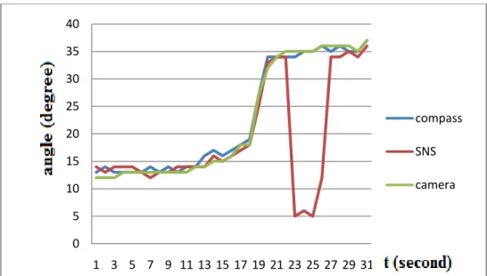
Fig. 4 shows an example of the work of diagnosis and recovery of the GPS signal. The figure clearly shows that during the 4 minute flight a mismatch between the SNS, a magnetometer and a camera testimony was observed. The failure was discovered and restored during one cycle of system calculation (200 ms).
0 5 10 15 20 25 30 35 40 1 3 5 7 9 11 13 15 17 19 21 23 25 27 29 31 angl e compass SNS camera
©UBMA - 2018
Figure.4 Image of a failure in the SNS with temporary loss of satellites and the result of the diagnosis Figure 5 shows three values of the heading angle obtained from the SNS, the optical system, and inertial sensors. It is clearly seen from the figure that a strong mismatch of signals appears at the 22nd second. The system has implemented a search for a fault location.
Figure.5 Checking results of the SNS system measurement after recovery
Using the methods of recovering the failed parameters described above in the article, the process of restoring the SNS indications was implemented. The parameters to be restored are the latitude, longitude and altitude of the aircraft.
The Fig.6 shows the experiment with the compass failure simulation. In this experiment, the failure is supposed to be specifically in a magnetometer. 0 0,2 0,4 0,6 0,8 1 1,2 1 3 5 7 9 11 13 15 17 19 21 23 25 27 29 31 failure 0 5 10 15 20 25 30 35 40 1 3 5 7 9 11 13 15 17 19 21 23 25 27 29 31 compass camera SNS with corrections
Figure.6 Image of a failure in the compass with temporary break in power
Figure.7 Checking results of the magnetometer after recovery The experimental results show the practical usefulness of this system in existing control systems.
As shown in the graphs, during the entire period of failure, the system was restoring value of the distorted channel with permissible precision (less than 3%).
This algorithm can identify the presence, time and place of failure.The negative quality is the necessity for 0 10 20 30 40 50 60 70 80 1 3 5 7 9 11 13 15 17 19 21 23 25 27 29 31 an gl e compass camera SNS 0 0,2 0,4 0,6 0,8 1 1,2 1 3 5 7 9 11 13 15 17 19 21 23 25 27 29 31 failure 0 10 20 30 40 50 60 70 80 1 3 5 7 9 11 13 15 17 19 21 23 25 27 29 31 compass with correction SNS camera
©UBMA - 2018 5. DISCUSSION
The positive qualities of this development is the operation speed in diagnosing, lack of long-term adaptation process to calculate the correct value of the failed channel, as well as the fact that this system is designed for a standard set of measuring devices, which are mounted on board of all modern autonomous aircraft. It makes the system particularly relevant on the world market.
At this stage of development it addressed the issue of the introduction of fuzzy logic algorithms to identify the location and type of failure of the accelerometer. This is due to the inefficiency of the classic line-up of sensors for solving this problem.
6. CONCLUSION
The main contribution of the paper is the idea of resource selection for system recovery without loss of stability and controllability. This is possible through a system approach to diagnosis and recovery systems. On this basis developed a series of algorithms can be represented as a dichotomous tree. These algorithms are easy to implement on any type of controllers. Thus, such principles and algorithms allow increase of efficiency of fault system recovery.
Development is relevant and in demand due to system features, associated with the flexibility of introduction to modern control systems. Introduction of this system does not require any reconstruction or transformations. This greatly reduces the cost of its installation in existing aircraft.
LITERATURE
[1] RaspopovV.Y., (2010) Microsystem Avionics ,.Ed Tula-Grif i K,Russia,168-219.
[2] Firsov S.N., (2014) Hardware-software complex for experimental tests of control processes and diagnostics of small spacecraft’s faults , Devices and systems. Management, monitoring, diagnostics, Vol. 6, 60 – 69.
[3] DybskaI., (2007) Robust control of the dosing member of turbine engine of aircraft on the basis of the dynamic perturbation compensator, Aerospace Engineering and Technology,Vol. 2, 20 – 24.
[4] KulikA.S., (2011) Active fault tolerance of satellite orientation and stabilization systems, Proceedings of the 10th International Conference of Iranian Aerospace Society, 25-26.
[5] ManiK.C., (2007) Fault tolerant systems, Morgan Kaufmann Publishers is an imprint of Elsevier, U.S.A., 17-20.
[6] Arif S., MuratA., (2015) Fault Tolerance Mechanisms in Distributed Systems, Int. J. Communications, Network and System Sciences, Vol. 8, 471-482.
[7] Nazirov R., (2010) Technical vision in control systems for mobile objects-2010, Proceedings of the scientific and technical conference-seminar, 4p.
[8] Lee P., Jeffrey M., Paul M., Alfons G., (2004) PVS specifications and proofs for fault-tolerant distributed system verification, available at the site internet : http://shemesh.larc.nasa.gov/fm/spider/ tphols2004/pvs.html.
[9] Hussain A., Alireza S., (2004) Fault tolerance for multiprocessor systems via time redundant task scheduling, Department of Electrical & Computer Engineering University of California Davis, U.S.A.
[10] Frank P., (1996) Analytical and qualitative model–based fault diagnosis – A survey and some new results.European Journal Of Control. Vol.2, 6-28
[11] Isermann R., Balle P., (1997) Trends in the applications of model-based fault detection and diagnosis of technical processes. Control Engineering Practice, N° 5, Vol. 5, 709–719