HAL Id: hal-02337105
https://hal.archives-ouvertes.fr/hal-02337105
Submitted on 29 Oct 2019
HAL is a multi-disciplinary open access
archive for the deposit and dissemination of
sci-entific research documents, whether they are
pub-lished or not. The documents may come from
teaching and research institutions in France or
abroad, or from public or private research centers.
L’archive ouverte pluridisciplinaire HAL, est
destinée au dépôt et à la diffusion de documents
scientifiques de niveau recherche, publiés ou non,
émanant des établissements d’enseignement et de
recherche français ou étrangers, des laboratoires
publics ou privés.
Hydrodynamics and SPM transport in an engineered
tidal estuary: the Adour river (France)
Sophie Defontaine, Damien Sous, Denis Morichon, Romaric Verney, Mathilde
Monperrus
To cite this version:
Sophie Defontaine, Damien Sous, Denis Morichon, Romaric Verney, Mathilde Monperrus.
Hydro-dynamics and SPM transport in an engineered tidal estuary: the Adour river (France). Estuarine,
Coastal and Shelf Science, Elsevier, 2019, pp.106445. �10.1016/j.ecss.2019.106445�. �hal-02337105�
Hydrodynamics and SPM transport in an engineered tidal estuary: the
1
Adour river (France)
2
Sophie Defontaine(a), Damien Sous(b,c), Denis Morichon(c), Romaric Verney(d), Mathilde
3
Monperrus(e)
4
(a)CNRS / Univ. Pau & Pays Adour/ E2S UPPA, Laboratoire de Mathématiques et de leurs Applications de Pau
5
- Fédération MIRA, UMR5142 64000, Pau, France
6
(b)Université de Toulon, Aix Marseille Université, CNRS, IRD, Mediterranean Institute of Oceanography (MIO),
7
La Garde, France
8
(c)Univ. Pau & Pays Adour / E2S UPPA, Laboratoire des Sciences de l’Ingénieur Appliquées à la Mécanique et
9
au Génie Electrique (SIAME) - MIRA, EA4581, 64600, Anglet, France
10
(d) IFREMER, DYNECO/DHYSED, CS10070, 29280 Plouzané, France
11
(e)CNRS / Univ. Pau & Pays Adour/ E2S UPPA, Institut des Sciences Analytiques et de Physico-Chimie pour
12
l’Environnement et les Matériaux - Fédération MIRA, UMR5254, 64600, Anglet, France
13
Abstract 14
The present paper reports on a series of field experiments aiming to characterise the functioning 15
of a man-engineered strongly forced salt-wedge estuary : the lower estuary of the Adour river, 16
France. Bottom-moored velocity measurements and surface boat surveys have been performed 17
under low river discharge conditions, for both neap and spring tides, in order to provide a well-18
documented reference framework to understand the dynamics of water masses, turbulence and 19
suspended particulate matter (SPM) transport in the lower estuary. An additional campaign has 20
been carried out in high river discharge conditions. This first documented in-situ study of the 21
Adour lower estuary demonstrates its variability in terms of hydrological regimes, from salt-wedge to 22
partially mixed regimes depending on tidal and discharge conditions. Turbulent properties showed 23
a significant response to the variations of salinity structure, with higher values when stratification 24
is minimal. At spring tide, a tidal variation between mixing conditions on the ebb and the flood 25
is revealed by ADCP measurements, with higher values extended up to the surface during the 26
ebb. The link between turbulent mixing and suspended sediment concentration is straightforward 27
during the ebb. During the flood, the suspended sediment concentration (SSC) seems related to 28
the salt-wedge entrance re-suspension and stratification-induced turbulence damping. No stable 29
Estuarine Turbidity Maximum (ETM) has been observed during the field experiment in the lower 30
Adour estuary. 31
Keywords: Salt-wedge estuary, estuarine circulation, stratification, turbulence, suspended 32
particles transport, Adour river. 33
1. Introduction 34
Estuaries are complex transfer areas of water masses and suspended particulate matters (SPM) 35
between ocean, land and continental waters [12]. They constitute unique habitats for a large variety 36
of living organisms and essential nurseries for many marine species. In the overall context of climate 37
change and growing anthropogenic pressure, a key issue of the preservation of estuarine ecosystems 38
is to improve our knowledge of the hydro-dynamical processes controlling the dynamics and renewal 39
of water masses in estuaries and their ability to transport, expel or retain sediments, contaminants, 40
nutrients and living organisms. 41
Many studies investigated estuarine dynamics from in-situ measurements [16, 46, 10, 44] and/ 42
or numerical modelling [32, 5, 41, 9]. From a physical point of view, estuaries are exchange areas 43
between fresh brackish continental water and salty marine waters, mainly driven by river run-off, 44
tides and wind forcing. Density gradients generated by the continental waters inter-playing with 45
marine waters, and interactions between tides and estuarine morphology have been shown to be 46
the major mechanisms governing the estuarine dynamics. Those mechanisms are known as : (i) 47
gravitational circulation induced by horizontal density gradient, (ii) tidal pumping generated by an 48
ebb-flood asymmetry, (iii) tidal straining caused by advection. The vertical salinity gradient plays 49
also an essential role by influencing the turbulent mixing inside the water column. Note that a 50
wide number of additional processes can also act on the estuarine dynamics and mixing, including 51
bed morphology [16], lateral circulation [13, 14, 31, 32, 45], wind [43, 40], Earth rotation [32, 56], 52
internal waves [54, 14, 15] and sediment load [61]. 53
A growing interest in classifying estuaries developed along the years, in order to gain a unified 54
view of the physics of estuaries. Different classification schemes have been proposed based on water 55
balance, geomorphology [39], vertical salinity structure [7] or hydrodynamics [24, 56, 21]. One of 56
the commonly used classification has been proposed by Cameron and Pritchard [7]. It is based on 57
water column stratification, in which estuaries can be classified as salt-wedge, strongly stratified, 58
weakly stratified or well mixed. However, the horizontal and vertical salinity gradients can show 59
important variations in time (e.g. from neap to spring tide, or from wet to dry season) and space 60
within a given estuary, such as stratification might not be systematically used to classify estuaries. 61
Therefore this type of qualitative classification has been progressively forsaken, to be replaced by 62
more quantitative methods. One recent approach has been proposed by Geyer and MacCready [21], 63
discussing the respective contributions of tide and river flow in mixing and stratification processes. 64
It is based on two dimensionless parameters. The former is the freshwater Froude number F rf [17]
65
which express the ratio between the river flow inertia and the buoyancy due to salinity gradient. The 66
second is the mixing parameter M which quantifies the effectiveness of tidal mixing in stratified 67
estuaries. Geyer and MacCready proposed a mapping of various estuaries based on those two 68
parameters, demonstrating the efficiency to discriminate different classes of estuary. For example, 69
salt-wedge estuaries, such as the Mississippi, The Fraser and the Ebro rivers are located near the 70
top of the F rf/M diagram (i.e. high values of F rf); while partially stratified estuaries are on the
71
center of the diagram (e.g. James river and San Fransisco Bay) and fjords and well mixed estuaries 72
are on the bottom part (e.g. Puget Sound). This research effort for a quantitative classification of 73
estuaries needs to be deepened and sustained, in particular by providing relevant in-situ data from 74
additional and contrasted case studies. 75
In addition to the hydrodynamic structure, a major issue of estuarine dynamics is to understand 76
the fate of the sediment load. Under the competing effects of turbulent suspension and gravitational 77
settling, strong variations of Suspended Particulate Matter (SPM) concentrations are observed in 78
both time, along the tidal cycle, and space, along the estuary [58, 18]. In the past decades, many
79
studies, see e.g. [9, 52, 4], have revealed the presence and the mechanisms responsible for the
80
generation of a zone of high turbidity, the so-called Estuarine Turbidity Maximum (ETM) in
salt-81
wedge estuaries. Three major mechanisms have been highlighted in the formation of ETM. First, 82
the estuarine circulation, due to longitudinal salinity gradient, associated with the river run-off drive 83
a convergent SPM transport at the salt intrusion limit, that can lead to the formation of an ETM. 84
Second, the asymmetry between the ebb and flood duration and peak velocities can also contribute 85
to the formation of an ETM. Third, damping of turbulent mixing, due to stable stratification, can 86
also be responsible for a sinking of particles from the upper part of the water column to the lower 87
part. Those particles will then be advected upward by the lower layer. In addition, a recent study 88
[23] also revealed that energetic wave conditions can influence the ETM mass by increasing the 89
mass by a factor of 3 during mean tides. The presence or the absence of an ETM in a given estuary 90
is a major concern when trying to understand and predict the dispersion or the retention of SPM 91
and related biochemical issues. 92
A significant research effort has thus been engaged during the last two decades to perform field 93
observations of turbulence, mixing and stratification in order to provide a basis for theoretical 94
analysis and numerical modelling of estuarine dynamics and sediment transport [49, 50, 48, 5, 21]. 95
The present study has been specifically designed to advance knowledge on hydrodynamics and 96
sediment transport in a man-engineered channel-shape estuary, subjected to strong tidal and fluvial 97
forcing, with few intertidal area and small watershed; as very few is known about such estuaries. 98
The selected field site is the Adour river estuary, located at the bottom of the Bay of Biscay. It is 99
a highly developed estuary with several kilometres of its downstream part completely channelised 100
in order to secure the Bayonne harbour operations. This specific morphology is reinforced by a 101
man-engineered reduction of the section at the last reach, in order to ease the expulsion of water 102
and sediment. The dynamics of estuarine water masses and sediments is further affected by human 103
interventions aiming to facilitate the navigation by dredging activities and wave protection. In 104
addition to this very specific morphology, the Adour estuary is also subjected to important fluvial 105
and tidal forcing, due to the location nearby the Pyrénées (heavy rainfall and snow melt freshet) and 106
the Atlantic ocean. Despite serious economic and environmental issues related to water quality and 107
sediment supply, very little is known about the functioning of the Adour estuary and the influence 108
of human interventions on its internal dynamics. Most known studies have focused on the dynamics 109
of the turbid plume and its area of influence in ocean waters [2, 11, 8, 37, 28]. 110
The aim of our study is to gain a detailed insight on the behaviour of the current and salinity 111
structure within the Adour river and their influence on particle matters dynamics. The present 112
paper reports therefore on the first field experimentation conducted in the lower Adour estuary, 113
where the marine waters play a primary role and the hydrological system remains simple enough 114
to be monitored. The methods and instrumentation are presented in section 2. The results are 115
detailed in section 3 and discussed in section 4. The last section is devoted to the conclusion. 116
2. Study site and data set 117
2.1. Study site 118
The Adour river originates in the Pyrenées mountains at an altitude of 2200 m, and flows about 119
300 km before pouring into the Bay of Biscay (SW of France). The catchment area is of about 120
17000 km2. The annual average river discharge is of about 300 m3.s−1, and can reach up to more 121
than 3 000 m3.s−1 during extreme flood events. The Adour river is characterised by a turbulent
122
pulsed transport with about 75 % of annual solid flux exported within 30-40 days [38]. The estuary 123
is exposed to a mesotidal regime, with a tidal range varying between 1 m to 4.5 m. The tidal regime 124
is mostly composed of semi-diurnal components (M2: 1.22 m, S2: 0.42 m, N2: 0.25 m, K2: 0.12 125
m). The tide wave propagates until St Vincent-de-Paul (70 km upstream), and the saline intrusion 126
limit is nearby Urt village (22 km upstream). The lower Adour river estuary (i.e. the lower 6 km), 127
which is our zone of primary interest, is a fully man-engineered channel of 150 m to 400 m width. 128
The main channel depth is maintained by dredging to about 10 m depth along the dock in the 129
Bayonne harbour, to ease navigation. The estuary mouth has been straightened and channelised 130
by embankments in order to accelerate water flow and to facilitate the sediment expulsion out of 131
the estuary. In addition, a 700 meters long jetty has been constructed at the north side of the river 132
mouth to protect the Bayonne harbour from swells mainly coming from the northwest sector (Fig. 133
1). 134
1 km
Convergent
Boucau
BSS
Quai de
Lesse s
−32 −28 −24 −20 −16 −12 −8 −4 0Bed
lev
el (m
)
2 kmAdour
Nive
Convergent
Boucau
BSS
Urt
Quai de Lesse s
-25 -25 -20 -15 Adour estuary FRANCE a) b) c)Figure 1:a) The study area, i.e. the last 6km of the estuary , with the Bayonne Harbor in blue. b) The location of the Adour estuary along the French coast. c) The Adour estuary from the entrance to Urt village. BSS white star is the boat survey station location. Boucau, Convergent, Quai de Lesseps and Urt white stars are the tide gauges locations. Colors represent the bathymetry in meter below the chart datum.
2.2. Field experiments 135
The objective of the present field experiments is to study the tidally-driven hydrodynamics 136
inside the lower estuary, including salt-wedge, stratification, mixing and SPM dynamics. The field 137
campaigns are based on a series of operations aiming to investigate the effect of river discharge and 138
tidal range on the estuarine dynamics. For the sake of simplicity, the experimental results will be 139
organized and named following the forcing conditions: LD/HD will refer to low/high river discharge 140
and ST/NT will refer to spring/neap tide conditions, respectively, while the year is added at the 141
end. For instance, LD-ST17 will refer to data recover in low discharge and spring tide conditions 142
in 2017. A summary of conditions during the boat survey measurements is given in Table 1, while 143
each type of measurement is described herebelow. The measurements have been undertaken only 144
in the last 6km of the estuary, in between the mouth and the confluence with the Nive river (Fig. 145 1 b)). 146 Conditions Date T.R. (m) Disch. (m3/s) LD-ST17 Sept, 19-20 2017 3.2-3.8 84-86 LD-NT17 Sept, 28-29 2017 1.2-1.3 112-128 LD-ST18 Sept, 25 2018 3.3 103 HD-ST18 June, 12 2018 3.2 1421
Table 1: Experimental conditions. LD/HD refer to low/high discharge conditions, respectively. ST/NT refer to spring/neap tide, respectively. T.R. and Disch. are the tidal range and river discharge, respectively.
2.2.1. Bottom moored measurements 147
A bottom-moored station has been deployed, at about 5 km from the entrance of the estuary, 148
at the same location than the boat survey station (BSS on Fig. 1), in September 2017. Velocity 149
profiles were recorded by a Flowquest ADCP (600 kHz) every 15 min (time averaged 5-min burst 150
data at 4Hz), with a vertical resolution of 0.5m. The ADCP was located at 0.56 m above the bed. 151
Velocity profiles recorded during LD-NT17 are presented in figure 4. 152
2.2.2. Fixed boat surveys 153
The fixed boat surveys were dedicated to the vertical structure of velocity, salinity, temperature 154
and turbidity. Measurements were performed from an anchored boat (BSS on Fig. 1). 155
The salinity, temperature and turbidity measurements were carried out by a Seabird C19plus 156
CTD sensor or a YSI 6920 probe. For each experiment, five-litre water samples have been taken 157
to calibrate the instruments. Forty kilograms weights were attached to the measurements line in 158
order to ensure the verticality. Probes measurements were recorded at 4Hz for the Seabird C19plus 159
and 1Hz for the YSI 6920. Temperature data will not be discussed in this paper, due to negligible 160
contributions in the density variations compared to salinity effect. 161
In addition to water properties measurements (1 profile every 15 min), high-frequency velocity 162
profiles were recorded, for LD-ST18 and HD-ST18 only, by a Nortek Signature 1000 current profiler 163
(ADCP) secured along the hull. The ADCP was continuously sampling at a rate of 8Hz with 20 to 164
30 cm cells. 165
2.2.3. Longitudinal sections 166
Longitudinal transects were realised across the control area (from 1 km to 5.5 km, from the 167
entrance of the estuary) with an OSIL Minibat under-water towed vehicle, equipped with a multi-168
parameter probe. Salinity, temperature, pressure and turbidity have been recorded by the Minibat. 169
Deployments have been carried out during LD-ST17 and LD-NT17 experiments (see Fig. 3 and 170
5, respectively). While the Minibat provides useful spatial information, its deployment remains a 171
very delicate operation in such a shallow and vertically sheared navigation channel. The transects 172
were surveyed following the centre axis of the estuary, i.e. not always in the main channel due to 173
navigation constraints near the docks. 174
2.2.4. Water levels 175
The tide gauge data presented hereafter have been collected either by Convergent or Bayonne-176
Boucau tide gauges, due to episodic malfunctioning. Both are operated by the Service Hydro-177
graphique et Océanographique de la Marine (SHOM) and located near to the entrance of the 178
estuary (Fig. 1). In this paper, those data will be presented in water elevation above the local 179
chart datum (in m C.D.). 180
2.3. Data processing 181
2.3.1. Velocity measurements 182
For each profiler, the velocity data are projected into a local coordinate system with the x axis 183
directed along the channel with positive values landward, the y axis directed laterally towards the 184
right bank, and the z axis directed upward. For simplicity, the generic term "velocity" generally 185
refers later on to the x-component of velocity, otherwise clarification will be given. 186
High frequency velocity data from LD-ST18 and HD-ST18 are used to analyse turbulence prop-187
erties. The 8Hz, 1s averaged, ADCP data of opposing beams (bi) have been split into a mean (bi)
188
and a fluctuating part (b0i), using a sampling interval of 10 min. An additional high-pass filter is 189
applied to remove low frequency fluctuations due to ship motion. The along-beam velocities have 190
been used to estimate the components of Reynolds stress [34, 60, 46], as follows : 191 −u0w0 = b 02 3 − b021 4sin(θ)cos(θ) (1) −v0w0= b 02 2 − b024 4sin(θ)cos(θ) (2)
where θ represent the angle of each beam from the axis of the instrument (θ = 25o for Nortek
192
Signature 1000 ADCP). 193
The eddy viscosity is classically computed following the flux-gradient hypothesis: 194
νt= −
u0w0
∂u/∂z (3)
The rate of Turbulent Kinetic Energy (TKE) production is expressed as a product of stress and 195 shear : 196 P = −ρu0w0∂u ∂z − ρv 0w0∂v ∂z (4) 2.3.2. Richardson number 197
The non-dimensional Richardson number Ri is often used to quantify the stability of the density 198
stratification in sheared flow [53]. A threshold value of 0.25 is commonly applied to distinguish stable 199
stratification from unstable situation due to the breakdown of stratification by turbulent mixing. 200
For high values of Ri, the buoyancy forces driven by the vertical density gradient are expected to 201
overcome and suppress turbulent mixing. The Richardson number formulation is here calculated 202
from the ratio between density and mean velocity gradients: 203
Ri = − g ρ0
∂ρ/∂z
(∂u/∂z)2 (5)
where ρ0 is the depth-averaged density. For the calculation of the Richardson number, density
204
is estimated according to UNESCO formula and density profiles are interpolated over the ADCP 205
regular measurement positions. It should be noted that in figure 2, the top of the water column is 206
missing in some salinity and SSC profiles due to the malfunctioning of our multi-parameters probe. 207
2.3.3. Turbidity and SSC 208
Turbidity profiles from boat surveys during LD-NT17, LD-ST18 and HD-ST18 have been con-209
verted into suspended sediment concentration (SSC) using a series of five-litre water samples and 210
pre-weighted glass fiber filters. 211
3. Results 212
The presentation of the field results will first focus on salinity structure and circulation, based on 213
the time evolution of the vertical profiles of the measured parameters (Figs. 2, 4 and 6 for LD-ST18, 214
LD-NT17 and HD-ST18 cases, respectively) together with longitudinal sections (Figs. 3 and 5 for 215
LD-ST17 and LD-NT17 cases, respectively). The LD-ST18 and HD-ST18 data are also depicted as 216
temporal contour plots in Figures 7 and 8, respectively. For theses cases, additional turbulence data 217
over the whole water column, including estimates of eddy viscosity and rate of TKE production, 218
are then presented from hull-mounted ADCP measurements, to analyse the competition between 219
turbulence and stratification. SPM dynamics is finally explored in the view of previous observations 220
on estuarine dynamics. 221
3.1. Estuarine salinity structure and circulation 222
Figures 2, 4, and 6 present the tidal evolution of velocity, salinity and Suspended Sediment 223
Concentration (SSC) profiles, during the dry season, for spring (LD-ST18) and neap (LD-NT17) 224
tide conditions, and during the wet season for spring tide (HD-ST18) respectively. Figures 3 and 225
5 display vertical salinity and turbidity structure along the last 6 km of the estuary, from Minibat 226
measurement during LD-ST17 and LD-NT17 experiments, respectively. 227
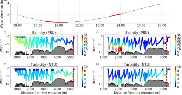
The data analysis is first focused on the spring tide condition during the dry season (Fig. 2 228
and 3). The ebbing tide is characterised by a horizontal salinity gradient (Fig. 2 (c) and Fig. 3 229
(b)), with a homogeneous water column flowing out the estuary. As the ebb progresses, the water 230
column becomes fresher and flows faster. At low water (11:36), the seaward current shows a strongly 231
sheared structure, with a nearly linear profile across the water column. Progressively, the water 232
column slows down and the salinity still decreases homogeneously along the water column. As the 233
tide rises, the salinity at the top of the water column goes on decreasing, while, at the bottom of 234
the water column the salinity increases. Salinity profiles are not homogeneous anymore, and the 235
salinity gradient increases. The current reversal occurred around 13:30 (i.e. almost 2 h lagged from 236
the low water time). The velocity profile reveals a typical salt-wedge profile, when the salty marine 237
waters flow into the estuary. A fast landward salty bottom layer is observed in the lower 3m, while 238
an oppositely fresh upper layer is still flowing seaward with a sheared profile. The salinity reaches 239
its minimal value in the surface layer, when the salt-wedge starts entering the estuary. The salty 240
bottom layer, which is rather well-mixed, increases both in thickness and salinity as the tide rises. 241
At the end of the flood tide, the full water column is salty and flows upstream, blocking the fresh 242
water inside the upper part of the estuary. The continental waters blocked into the upper part of 243
the estuary during the flood, are then released during the ebb. This mechanism, named "pulsed 244
plume mechanism", has already been highlighted by Dailloux [8]. 245
Figure 2: Tidal dynamics from LD-ST18 fixed boat surveys during low discharge spring tide conditions. (a) Water level and timing of measurements. (b), (c), and (d): velocity, salinity and SSC profiles. Note that the same data is presented in contour plots in Figure 7.
Figure 3: Longitudinal and vertical structure across the lower estuary from Minibat measurement during LD-ST17 experiment. (a): Water elevation with measurement periods highlighted in red. (b) and (c): salinity data for falling and rising tide. (d) and (e): turbidity data for falling and rising tide. The bed of the estuary is represented in grey. The red dashed line represents the BSS location.
The contrast between spring tide and neap tide (Fig. 4 and 5) is straightforward, as during neap 246
tide the salinity stratification is maintained all along the tidal cycle and the velocity magnitudes are 247
reduced. At the end of the flood (11:00), a sharp pycnocline separates a two-layer flow, with denser 248
marine water flowing upstream underneath fresh continental waters. The bottom saline layer grows 249
thicker until post-high tide slack water (14:00). Unlike spring tide, at neap tide the pycnocline is not 250
able to reach the surface. The current reversal is lagged of almost 3h from the high water (10:49). 251
As flow reverses seaward, the pycnocline thickens and deepens, while the surface and the bottom 252
salinity remain relatively constant. This time the ebbing shear velocity profiles are associated with 253
a vertical stratification. This permanent stratification leading to an inhibition of the salt-wedge 254
flushing during neap tide is generally associated with stagnant waters and hypoxia [29, 3]. 255
Figure 4: Tidal dynamics from LD-NT17 fixed boat surveys during low discharge neap tide conditions. (a) Water level and timing of measurements. (b), (c), and (d): velocity, salinity and SSC profiles.
Figure 5: Longitudinal and vertical structure across the lower estuary from Minibat measurement during LD-NT17 experiment. (a): Water elevation with measurement periods highlighted in red. (b) and (c): salinity data for falling and rising tide. (d) and (e): turbidity data for falling and rising tide. The bed of the estuary is represented in grey. The red dashed line represents the BSS location.
A dedicated experiment (HD-ST18) was carried out during a high discharge event in order to 256
explore the role of river runoff on the hydro and sediment dynamics compared to the reference 257
low river discharge dataset presented hereabove. Figure 6 depicts the time evolution of velocity 258
profiles, salinity and Suspended Sediment Concentration (SSC) profiles during high river discharge 259
conditions. The comparison with low discharge conditions presented in Figure 2 shows the drastic 260
influence of river run-off on the estuarine dynamics. Similar maximal magnitudes are reached during 261
the ebb, but the velocity profile is almost constant, and the water column is homogeneously fresh. 262
As tide rises, the water column shows a piston-like behaviour, i.e. marine water impounding river 263
water into the estuary with a quasi uniform velocity along the vertical. The current reversal (13:00) 264
occurs much later for the high discharge case, i.e. almost three hours after the low water (09:58), 265
than for the low discharge case. The piston-like behaviour remains active all along the flow reversal 266
and during the most part of the flood tide. This greatly differs from the low discharge case for 267
which a vertical shear of velocity is systematic at the early stage of flood tide. At the very end of 268
the flood (16:00), the salt-wedge is finally able to reach the measurement area. A 2 m thick bottom 269
salty layer propagates upstream at about 0.5 m/s. The high river discharge is again responsible for 270
a significant time lag compared to low discharge conditions for which the salt-wedge was able to 271
reach boat survey station about 2 h earlier. A remarkable observation, at the salt-wedge arrival, is 272
the rapid seaward reversal of the overlying fresh water layer. The water column forms, therefore, 273
a two-layer vertical structure with strong vertical shear in velocity and a sharp pycnocline. Note 274
that the seaward/landward velocity maxima are reached in the upper parts of the pycnocline and 275
of the salt-wedge, respectively. 276
Figure 6: Tidal dynamics from HD-ST18 fixed boat surveys during high discharge spring tide conditions. (a) Water level and timing of measurements. (b), (c), and (d): velocity, salinity and SSC profiles. Note that the same data is presented in contour plots in Figure 8.
3.2. Turbulence properties 277
The previous section revealed the complex vertical salinity structure and circulation taking 278
place into the Adour estuary. This first result needs to be further investigated by a turbulent 279
properties analysis, to get a better understanding of the interaction between stratification and 280
turbulent mixing. The representation of Richardson number profile as log10(Ri/0.25) is used in
281
figures 7 and 8 to easily estimate the stability of the water column: stable (unstable) flows are 282
expected for positive (negative) values. In addition, high-resolution high-frequency velocity profiles 283
are used to infer turbulent properties of the flow. Figures 7 and 8 shows the tidal evolution of the 284
vertical distribution of turbulent properties at the survey station BSS for the low (LD-ST18) and 285
high (HD-ST18) river discharge experiments respectively. 286
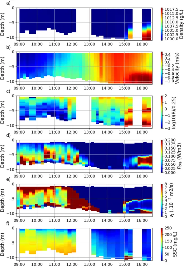
Figure 7 depicts the data recovered during spring tide and low discharge conditions (LD-ST18). 287
At 08:15, the water column is slightly stratified and the production of turbulence is focused in a 288
very thin layer above the bed related with weak turbulent diffusion in most of the water column. As 289
the water column becomes homogeneous and ebb current accelerates during the estuary flushing, 290
the turbulence spreads into the water column aside from in the 2 m surface layer. The turbulent 291
mixing overcomes the buoyancy forces and water column becomes fully unstable (log10(Ri/0.25) <
292
0). Maximal values of Ptkeand νtare associated with maximum ebb currents. The eddy viscosity
293
is maximal in the bottom 4 m and reaches typical values (about 1.5 10−2 m2.s−1) measured in 294
estuary for similar velocity and stratification conditions [46]. Those measurements also confirms 295
that the eddy viscosity decreases toward the surface [35]. The slack water and the subsequent flow 296
reversal are associated with a drastic drop of turbulence production. After 13:00, the sign change of 297
the Richardson number indicates the shift toward a stable stratified situation which further reduces 298
the eddy viscosity. At the salt-wedge entrance (around 13:30), a stable stratification develops with 299
no turbulent mixing except an increase of TKE production and eddy viscosity at the tip of the 300
salt-wedge. High values of Richardson number are associated to the edges of the pycnocline. Burst 301
of turbulent production seems to develop in the upper layer between 14:00 and 14:30, which may 302
correspond to a local destabilisation of the sheared layer. As the tide rises, the water column turns 303
on stable up to the surface with no more turbulent mixing. 304
Figure 7: Tidal evolution during LD-ST18 experiment : (a) vertical structure of density, (b) time-averaged velocity, (c) Richardson number, (d) production rate of TKE, (e) eddy viscosity, and (f) suspended sediment concentration.
In addition, Ri calculations (not shown here) have been carried out for neap tide conditions 305
based on profiles shown in figure 4. As expected, the nearly permanent vertical salinity stratification 306
promotes stability throughout the water column. 307
Figure 8 presents similar data than figure 7, but applied on data collected under high river 308
run-off conditions. It is first recalled that Richardson number should be considered with respect to 309
the corresponding velocity and density profiles: nearly neutrally stratified conditions (i.e. unstable 310
conditions) may appear stable in terms of Richardson number when the velocity shear is very weak. 311
This is for instance the case in the surface layer (Fig. 8). During high discharge conditions, the 312
lower estuary is filled with fresh water for most of the tidal cycle, the only exception being the salt-313
wedge arrival just before high tide (15:00). Therefore, the turbulent properties variations drastically 314
differ from the low discharge case shown in figure 7. At the end of the ebb tide (before 10:00), the 315
water column is fully fresh and has an almost constant velocity. High rate of TKE production and 316
eddy viscosity are measured at the peak of ebb currents. The strong discharge is able to maintain 317
the instability and a significant TKE production until 12:00 (i.e. more than two hours after low 318
tide). Then, slack water (around 13:00) is associated to a strong drop of turbulence production and 319
eddy viscosity, which remains very weak until the arrival of the salt-wedge. However, the piston 320
effect is clearly visible at rising, with nearly vertically uniform velocity profiles during most of the 321
rising tide. The consequence, in term of stability, is that the lower estuary remains unstable all 322
the time until the salt-wedge is able to reach the measurement station (15:00). A first moderate 323
rise of TKE production is observed near the bottom to a depth of 3m, which indicates that the 324
tip of the salt-wedge is a mixing zone. From that moment, one notes the development of a 1 to 325
2 m high pycnocline, both strongly stratified and very sheared. Corresponding positive values of 326
Richardson number indicates the stability of the sheared layer. Peaks of Richardson number are 327
observed near the edges of the pycnocline, associated to more stable areas, whereas the core of the 328
sheared zone is very close to the instability threshold. The TKE production strongly rises near 329
the bottom, but remains confined near the bottom layer by the effect of overlying stratification. 330
It can be noticed that, even if the velocity of entering marine waters is much lower than for the 331
low discharge case, a much stronger turbulent mixing is observed in the bottom layer. The salt-332
wedge arrival (15:00) is a striking example of a dynamical competition between turbulent mixing 333
and stratification: turbulent diffusion is very active near the bottom and below the pycnocline, but 334
totally vanishes in the overlying fresh water layer. 335
Figure 8: Tidal evolution during HD-ST18 experiment : (a) vertical structure of density, (b) time-averaged velocity, (c) Richardson number, (d) rate of TKE production, (e) eddy viscosity and (f) suspended sediment concentration. Note the difference in range compared to Figure 7.
3.3. Suspended sediment dynamics 336
This section is dedicated to the response of the sediment load to the complex hydrodynamics of 337
the lower Adour estuary presented above. Figures 2 (d), 4 (d) and 6 (d) represent the SSC profiles 338
collected during LD-ST18, LD-NT17 and HD-ST18 respectively. Figures 7 (f) and 8 (f) display 339
same data as presented in Figures 2 (d) and 6 (d) under timeseries color plots. Figures 3 (d), (e) 340
and 5 (d), (e) show Minibat turbidity data collected during LD-ST17 and LD-NT17 respectively. 341
First, a focus on the low river discharge reference case allow us to study the effect of tidalcycle
342
on sediment dynamics, such as erosion, advection and deposition mechanisms. In Figures 2 and 7,
343
it can be noticed that at mid-ebb, the full water column is flowing out the estuary and the vertical
344
velocity gradient is increasing. It results in a sufficient bottom shear stress to re-suspend sediment
345
around 08:30. The sediments are maintained in suspension and are able to reach the surface of
346
the water column by the turbulent mixing appearing at 09:00. Figure 3 shows that a horizontal 347
gradient of SSC associated to the horizontal gradient of salinity develops, with SSC increasing as 348
the water becomes fresher. These sediments in suspension are advected seaward by the flow, at
349
a velocity that can reach 1.5 m.s−1 in the surface. Approaching the slack water period (12:00), 350
the ebbing velocity is less than 0.6 m/s (green profiles on Fig. 7) and the vertical gradient of
351
velocity decreases. Consequently the re-suspension capacity of the flow decreases. The turbulence
352
maintaining the sediment in suspension also drops down, and sothe SSC develops a vertical gradient, 353
which might be associated to settling. It progressively leads to an overall SSC decrease. Around
354
14:00, sediments accumulated at the bottom of the water column are advected landward by the
355
entrance of the marine waters into the estuary, while sediments located at the surface are still
356
advected seaward. At 15:00, an area of high turbidity is generated at the tip of the salt-wedge 357
front. This trend is generally attributed to the accumulation of sedimentsdue to the convergence
358
of sediment fluxes from the river and the ocean. This peak of SSC is contained near the bottom by
359
the pycnocline. Another striking feature is the decrease of SSC in the layer of fresh continental water 360
flowing above the salt-wedge (Fig. 7 and 3). This observation should likely be attributed to the 361
stratification-induced damping of turbulence, leading to particles sinking, as previously observed in 362
other systems [59, 18]. At 16:00, velocity profiles are much more homogeneous and the turbulence
363
is damped by the stability of the two-layer flow, and so the SSC decreases.
364
The tidal range has also a striking effect on the above mentioned sediment dynamics, as shown
365
by the comparison between Figures 2 and 4. During neap tides,the SSC remains very low, about 10 366
mg.L−1 all over the tidal cycle and quite homogeneous over the water column,while during spring
367
tides,the SSC is generally stronger (up to 45 mg.L−1) and slightly more variable throughout the
368
tidal cycle. This very low SSC can be explained by a permanent stratification and a reduced
369
velocity. Low velocities impede the re-suspension of sediments and the permanent stratification
370
damps down the turbulence. The sediments can therefore not remain in suspension. During neap
371
tides the flushing capacity is drastically reduced by the absence of re-suspension and advection and
372
the strong deposition.
373
The riverine forcing also influences the sediment dynamics, as highlighted by Figures 6 and 8.
374
During high river discharge, the ebbing currents are reinforced and the flow is much more turbulent,
375
resulting in a stronger re-suspension and seaward advection. Consequently, SSC values are much 376
more higher than those observed during low discharge conditions. In Figure 8, it can be noticed
377
that during the ebb, the SSC is quite homogeneous in the water column, with values about 150 378
mg.L−1. These reinforced re-suspension and advection result in a very good flushing capacity of
379
the estuary. At 11:30, both flow and turbulent mixing reduce in intensity. The particles are not
380
anymore maintained in suspension and a progressive sedimentation can be observed. The SSC
381
shows a pattern similar to the one of turbulent properties. Between 15:00 and 17:00, the
piston-382
like behaviour occurs pushing slowly the full low SSC water column landward. Similarly to the
383
low discharge conditions,the salt-wedge passing (15:00) corresponds to the higher measured SSC. 384
However, during high river discharge, the SSC is able to reach up to 850 mg.L−1 in the bottom
385
layer. The increased river flow reinforces the convergence mechanism. These sediment in suspension
386
are also contained by the pycnocline and advected landward, while the surface waters containing
387
little sediments are advected seaward. Around one hour after the salt-wedge front passing, the SSC 388
at the bottom of the water column has decreased to about 100 mg.L−1. This high turbidity area 389
is thus supposed to follow the up estuary motion of the salt-wedge leading front. 390
4. Discussion 391
This article presents a set of field observations carried out to improve the knowledge about 392
circulation and sediment transport into the lower Adour estuary. These results provide the first 393
in-situ characterisation of the hydrological functioning of the Adour lower estuary, but also give rise 394
to a number of questions. Discussion points have been organised under three main topics: estuarine 395
salinity structure and circulation, sediment dynamics and connection to plume dynamics. 396
4.1. Estuarine circulation
397
The present in-situ dataset revealed the high variability of the Adour lower estuary, in terms 398
of hydrological functioning. A salt-wedge generally develops during the flood tide in the Adour 399
lower estuary. This salt-wedge depends on river discharge, by being more steeply marked during 400
the wet season due to intense river forcing. In addition, the tidal forcing is also an important driver 401
of the Adour estuary (mesotidal system) with a significant effect of the spring/neap cycles on the 402
estuarine salinity structure. Under low discharge conditions, the neap tides are associated to fully 403
vertically stratified estuary along the tidal cycle, while during spring tide the salt-wedge shape is 404
lost during the ebb, and an horizontal salinity gradient takes place. Such a versatility in the salinity 405
circulation in response to the fluctuations of tidal and fluvial forcing can not be properly accounted 406
for by usual descriptive estuary classifications, such as, e.g. the well-know scheme of Cameron and 407
Pritchard [7]. More physical insight is provided by the recent quantitative scheme of classification 408
developed by Geyer and MacCready [21]. 409
The scheme of classification developed by Geyer and MacCready [21] investigates the respective 410
contribution of tidal mixing and stratification by the means of a two parameters space : the freshwa-411
ter Froude number F rf = UR/(βgsoceanH)1/2and the mixing parameter M =p(CDUT2)/(ωN0H2),
412
where UR is the net velocity due to river flow (i.e. the river volume flux divided by the estuarine
413
section), β is the coefficient of saline contraction, g is the acceleration due to gravity, soceanis the
414
ocean salinity, H is the water depth, CD is the bottom drag coefficient, UT is the amplitude of the
415
tidal velocity, ω is the tidal frequency and N0 = (βgsocean/H)1/2 is the buoyancy frequency for
416
maximum top-to-bottom salinity variation in an estuary. The former dimensionless parameter F rf
417
compares the net velocity due to river flow and the maximum possible front propagation speed, 418
while the latter M assesses the role of tidal mixing and the influence of stratification on the vertical 419
mixing. Due to spring/neap variations and wet/dry seasons changes, estuaries are not represented 420
by a point in this classification scheme, but rather by rectangles covering the range of observed 421
regimes. An adaptation of the Geyer and MacCready’s regime diagram [21] is proposed in Figure 9, 422
with the M and F rf ranges reached by some well-documented estuarine systems in order to easily
423
compare with the Adour estuary. 424
Of particular interest is to know the extent to which the variability of the Adour estuary can 425
be described by such approach and to evaluate how it can compare to other typical systems 426
selected for their contrasted dynamics. For the calculation of both parameters, we considered 427
β = 7.710−4P SU−1, H to be a characteristic value of the water depth H = 10m, the salinity of
428
ocean socean = 34.5 PSU. A first remark should be made on the uncertainty on the estimation of
429
the mixing parameter M . This parameter shows a strong sensitivity to both UT and CD values,
430
which are not straightforward to estimate. In Geyer et al 2014 [21], UT is defined as the amplitude
431
of the depth-averaged tidal velocity, while it has been estimated as the rms velocity 3m above the 432
bed in Geyer et al 2000 [20] and considered equivalent to the maximal velocity in Li et al 2014 433
[33]. For the present study, the reference value of UT is provided by rms depth-averaged velocity
434
measured at the BSS bottom moored station (Fig. 1). The bottom drag coefficient CD can also
435
be strongly spatially variable inside an estuary, and relatively challenging to estimate. In Geyer et 436
al. 2014 [21] authors consider that CD generally varies between 1 to 2.5 10−3 inside an estuary,
437
while Geyer et al. 2010 [17] mentioned a value of CD generally about 3 10−3 inside estuaries. For
438
the Adour estuary, two point currentmeters deployed in the bottom layer have been used by Sous 439
et al [47] to estimate a CD value about 1.5 10−3 between Convergent and BSS stations, which is
440
used here as a reference for the estimation of M . Using data collected inside the Adour estuary, UR
441
estimation ranges from 0.05 to 0.75 m.s−1, therefore F rf should range from 0.03 to 0.46 for low to
442
high discharge conditions,respectively. The mixing parameter M , based on reference values for UT
443
and CD, ranges from 0.36 to 0.66 for neap to spring tide conditions, respectively (Fig. 9, solid line
444
rectangle). In order to illustrate the M sensitivity to UR and CD parameters, estimating now UT
445
as the maximal entering velocity together with a CD value of 3 10−3 will shift the Adour’s system
446
toward higher ranges of mixing parameter values (0.68 to 1.13), see dashed line rectangle in Figure 447
9. In addition, the values of the mixing parameter might be further increased with data from neap 448
tide conditions combined to high river run-off, which are not documented by the present dataset. 449
Keeping in mind these limitations, the estuarine parameter space diagram proposed by Geyer 450
and MacCready [21] confirms the variability of the hydrological functioning of the Adour estuary 451
in comparison with other typical systems (Fig. 9). Noted that the large area covered by the 452
Adour river in this diagram is due to the highly contrasted hydrological conditions encountered 453
during our measurements. Others systems may have been observed only during mean hydrological 454
conditions, leading to reduced rectangles. Based on collected data, presented in this paper, we 455
can analyse the observed dynamics of the Adour estuary. Under high tidal mixing conditions 456
(i.e. high M value), the Adour river dynamics is quite similar to those of Fraser [19], Changjiang 457
[33] and Merrimack rivers [41], which are all considered as time-dependent salt-wedge estuaries. 458
Those energetic and stratified estuaries are characterised by strong tidal and fluvial velocities (Fig. 459
10). It results in a strengthened stratification during the flood, that weakens during the ebb tide, 460
where the turbulence develops in the full water column. Under low tidal mixing conditions (i.e. 461
low M value), the Adour tends to show a behaviour similar to the Ebro river. This latter has a 462
similar shape and river discharge than the Adour, but the microtidal regime (associated to a small 463
M ) results in a stagnant salt-wedge under low river run-off ejected out of the estuary when the 464
river discharge exceeds 500 m3.s−1 [25]. Measurements undertaken during neap tide and low river
465
discharge in the Adour estuary reveal a similar pattern with an almost stagnant salt-wedge and 466
strong stratification. Unfortunately, observations were not carried out during neap tide and high 467
river discharge (around 1500 m3.s−1), but we can expect an absence of the salt-wedge or at least
468
a strong reduction of the saline intrusion. The role of river discharge is however clearly identified 469
for spring tides, corresponding to fluctuations along the F rf axis in Figure 9 for large value of M .
470
Under low river discharge conditions (i.e. low F rf value), the influence of tidal mixing is more
471
important, leading to a smoother vertical stratification and a strongly stratified regime. During the 472
ebb, the peak of turbulence can be sufficient to break down the vertical stratification and generate 473
an horizontal stratification. This horizontal stratification is a typical attribute of partially mixed 474
regime. When the river discharge increases (i.e. higher F rf values), the vertical stratification
475
appears to be stronger, with a sharper pycnocline and a salt-wedge restricted in the lower part of 476
the water column. 477
Figure 9: Estuarine classification based on the freshwater Froude number and mixing number, adapted from [21], Fig 6. (*) The dashed rectangle represent the location of the Adour river using other estimations of Ut and CD.
Figure 10: Tidally averaged velocity profiles for neap (full black line) and spring (full red line) tides with low river discharge. Flood (dotted lines) and ebb (dashed lines) average velocity profiles for neap/spring low river discharge conditions. Data from bottom moored station located at BSS location (Fig. 1)
The lateral dynamics, which has not been explored in the present data analysis, may play an 478
additional important role in the estuarine circulation and salinity structure. Both local curvature of 479
the lower estuary and cross-sectional bathymetric gradient are expected to favor a degree of three-480
dimensionality in the estuarine flow structure [31, 44]. This calls for further dedicated experimental 481
campaign to better understand the contributions of along-channel and lateral components in mixing 482
processes, and their dependencies on tidal range and river discharge. 483
4.2. Suspended sediment dynamics 484
The present study allows to analyse the impacts of physical processes taking place inside the 485
Adour estuary on the observed sediment transport. Since the Glangeaud’s pioneering description of 486
an Estuarine Turbidity Maximum (ETM) in the Gironde estuary in 1938 [22], a series of numerical 487
and experimental studies have revealed the importance of ETM in estuarine sediment dynamics 488
[4, 27, 55, 6] among others. ETM have strong impacts on the marine and estuarine ecosystems, 489
being a major driver of sediments, contaminants and nutrients from continent to ocean. ETM 490
formation is primarily driven by the hydrodynamical functioning of the estuary. In salt-wedge 491
systems, and in particular in the presence of strong tidal forcing, two key mechanisms have been 492
identified in the ETM dynamics: the residual gravitational circulation and the tidal asymmetry. 493
Burchard and Baumert [4] demonstrated that tidal asymmetry is of a bigger importance in the 494
ETM formation than gravitational circulation in macrotidal salt-wedge estuaries. The gravitational 495
circulation plays a part in sustaining and stabilising the ETM mass. In the Charente estuary, which 496
shows similarities with the Adour in terms of dimension and salt-wedge regime but with a stronger 497
tidal forcing, the tidal asymmetry is mostly responsible for the formation of the turbidity maximum, 498
while the density gradient has an influence on its shape and its stratification [52]. More recently, 499
Olabarrieta et al. [36] have highlighted the role of density gradient-driven subtidal flows in the 500
sediment import and trapping into the estuary associated to near-bed flood tide dominance. 501
Based on the present dataset, no stable ETM has been observed in the lower Adour estuary. 502
Further insight is provided by analysing the main expected ETM drivers. First, the tidal assymetry 503
in the Adour estuary has been studied based on the water elevations collected by tidal gauges 504
along the estuary. Figure 11 outlines that a slight tidal asymmetry of less than 20 minutes exists 505
in the lower estuary. Provided time lag appears too weak to generate an ETM when compared 506
to the Charente estuary, where tidal asymetry can reach almost 3.8h at the river mouth [52, 51]. 507
A strongest asymmetry can be noticed in the upper part of the estuary (i.e. 20 km upstream at 508
Urt village). Such mechanism might generate on ETM in this reach of the estuary. Extended 509
measurements until Urt village or a dedicated numerical study are foreseen as further work to 510
estimate the impact of this tidal asymmetry on the sediment transport in the upper estuary. The 511
second ETM driving process is the residual estuarine circulation. In most cases, no residual estuarine 512
circulation has been observed in the lower estuary. The mean ebbing velocities are stronger than 513
the mean flooding velocities, resulting in a good flushing of water masses and suspended sediment. 514
The only exception is observed during very low river flow and tidal forcing conditions, as revealed 515
by the residual tidally-averaged velocity profiles depicted in Figure 10, black solid line. In such 516
conditions, a residual circulation is observed, but its effect in generating a well-developped ETM is 517
likely compensated by limited resuspension due to reduced velocities. Note however that the bottom 518
moored current profilers are not able to resolve the bottom 1.5 m (structure size and blanking zone), 519
which can hide near-bed processes. 520
Moreover, it should be noted that riverine input of sediment is very low compared to other
521
tidal estuaries, based on SSC obtained in the present conditions. Even during high river discharge,
522
during the ebb, when the water column is full of fresh riverine waters flowing out the estuary, the
523
SSC is about 150 mg.L−1. This very low supply in sediment even during high river discharge might
524
be related to the marshy meadows located along the Adour river, which could be responsible for
525
particle trapping.
Figure 11: Water elevation data collected at Urt village (22 km from the estuary mouth, in magenta), at Convergent
(700 m from the estuary mouth,in black) and Quai de Lesseps (5.6 km from the estuary mouth, in bleu) tide gauges,
during spring tide.
The observed influence of tidal range on the lower estuary has also a strong effect on the ejected
527
plume. At spring tide during the dry season, continental waters are blocked inside the estuary by
528
the marine waters entrance for about three hours. This mechanism drives the pulsed behaviour
529
of the plume of the Adour estuary already highlighted by Dailloux [8]. By contrast, at neap tide
530
during low discharge conditions or under high discharge conditions, a layer of continental water is
531
flowing seaward all along the tidal cycle at the top of the water column, almost constantly feeding
532
the plume leaving the estuary with fresh water. The pulsed behaviour of the Adour estuary may
533
take place only when the tidal forcing is able to overcome the riverine forcing, and so the riverine
534
waters are blocked into the estuary by the marine water entrance.
535
4.3. Impacts of engineering works
536
The Adour estuary exhibits a strong variability of salinity, which has never been reported in the
537
literature. This is highlighted by direct measurements in a range of conditions and confirmed by 538
the Geyer and MacCready classification diagram [21]. Part of the observed variability is directly 539
imposed by the fluctuations of the external forcing, i.e. a mesotidal regime associated with seasonal 540
variations of river discharge driven by the oceanic climate and the close proximity to the Pyrenées 541
mountains. However, such conditions may not entirely explain the observed variability of estuarine 542
salinity circulation when comparing the Adour to other systems. It can be hypothesised that the 543
artificial channelisation of the lower estuary coupling with strong dredging activities act to enhance 544
the fluctuations in hydrological regimes. The Adour estuary is fully artificial since 1578, when the
545
mouth of the estuary has been fixed in front of the Bayonne city by diking, under the decision
546
of King Charles IX. In 1810, Napoleon decided to reduce the entrance of the estuary to 150 m
547
in the aim of protecting the channel from sand accumulation by focusing the ebb energy. For a 548
wider lower estuary, which would be likely the case in a more natural context, the UR value would
consequently decrease and so the F rf. This reduction of river flow velocity should reduce the
550
stratification within the estuary which should promote the development of strongly stratified or 551
partially mixed regimes. These engineering works are complemented by dredging activities from
552
1896. Nowadays, the quantity of sediments to be dredged in the lower estuary per year is about
553
525000 m3. The dredger of 1200 m3 capacity operates almost everyday, except from June to
554
September. Thisis also supposed to have a significant impact on the stratification, by maintaining 555
the channel deeper. In the absence of dredging, the depth reduction would strengthen the river flow 556
and decrease the tidal propagation speed, resulting in an enhanced mixing. Following the Geyer 557
and MacCready classification [21], this wouldresultin an increase of both parameters likely leading 558
to a more systematic time-dependent salt-wedge regime. Such assumptions can certainly not be 559
directly assessed from the presentor formerdataset, and would require prospective scenarios with 560
dedicated numerical modelling to be further discussed. The potential changes on estuarine salinity 561
structure might have significant consequences on biogeochemical processes controlled by mixing, 562
residence time and water properties. Such issues should obviously not only concern the Adour 563
system and call for a more extensive assessment of the impact of artificialisation and urbanisation 564
of estuarine systems on the physical processes controlling the hydrodynamics and finally affecting 565
the entire ecosystem. 566
The question arises then on the role of estuary engineering (channelisation and dredging) on 567
the absence of observed ETM in the lower reach of the estuary, in particular when compared to 568
othertidalestuaries. First, the width reduction at the estuary mouth certainly enhances the good 569
flushing capacity of the lower Adourby reinforcing the ebbing currents. Such hypothesis might be
570
impossible to confirm due to the lack of available data collected before those engineering works,
571
a numerical study could be necessary to discuss further this issue. In addition, it is hypothesized 572
that the artificialization of the river mouth tends to maintain a low marine sediment input, thus 573
participating to the absence of ETM. At the river mouth, along the Northern jetty, a sand pit has 574
been artificially created and maintained by dredging operations, in order to avoid sand accumulation 575
in the estuary entrance under storm conditions. Dubranna’s numerical study [11] highlighted that 576
the transport of sediment from the coastal area into the estuary is strongly limited by this man-577
engineered retention pit. Grasso and al [23] have shown the important contribution of energetic wave 578
conditions to the ETM mass, by sediment resuspension action. However, it has been demonstrated 579
that both jetties located at the estuary entrance, efficiently protect the port against incoming 580
swell and sea waves with a reduction factor of 85 % compared to the offshore wave energy [1]. 581
All together, these interventions may also contribute to the absence of ETM in the Adour lower 582
estuary. Nevertheless, the impacts of the artificialisation of the lower estuary on its hydrodynamics
583
and sediment transport can not be quantified by the present study, and would require further
584
investigations.
585
The plume generated by the brackish fresh waters flowing out the estuary is also influenced by
586
the engineering works at the entrance of the estuary. As already mentioned the width reduction at
587
the entrance of the estuary might be responsible for an intensification of the plume. In addition,
588
the Northern jetty also affects the dispersion of the plume orienting the plume in the southwest
589
direction. Such issue was not part of the scope of this study, however this could be the aim for
590
additional research. Additional measurements upstream in the Adour estuary would be necessary
591
to confirm such hypothesis.
5. Conclusion 593
This study aimed to investigate the hydro-sedimentary behaviour of the lower Adour estuary 594
by means of field experiments. A series of hydrodynamical processes are documented through 595
bottom-moored, hull-mounted and vertical profiling instrumentation. It has been shown that its 596
functioning is strongly influenced by both river and tidal forcing, resulting in a wide range of density 597
stratification. The stratification variations show different time scales : from flood to ebb tides, from 598
neap to spring tides, even from dry to wet seasons. It has been demonstrated that stratification is 599
strengthened during the flood tide and weakened during the ebb tide. During low river discharge, 600
neap tides promote stable salt-wedge in the lower estuary, while spring tides allow full flushing of 601
the salt-wedge. On the other hand, wet season has a tendency to constrain the salt-wedge in a thin 602
bottom layer, enhancing the vertical stratification. This strong variability in the flow structure has 603
a huge influence on the flushing capacity of the estuary. 604
The tidal evolution of the gradient of Richardson number has revealed the straight influence 605
of the salinity structure on the turbulent mixing. Flood tide is generally associated with reduced 606
turbulence production and stable stratification, while ebb tide is characterised by strong turbulent 607
mixing. Through stratification and mixing characteristics of the Adour estuary, a recent classifica-608
tion scheme has been applied to compare it to others salt-wedge estuaries. Based on the Geyer and 609
MacCready classification [21], the Adour estuary varies from salt-wedge to partially mixed estuary. 610
Density effects, salt-wedge displacement and the competition between stratification and mixing 611
processes have a strong impact on the suspended matter displacement : longitudinal convergence at 612
the salt tip, sinking of particles due to stratification induced turbulence damping, and re-suspension 613
due to the salt-wedge passing. However, both major mechanisms associated with ETM generation 614
have not been observed in the lower estuary : tidal asymmetry and residual estuarine circulation. 615
Acknowledgments 616
This study was sponsored by the EC2CO PANACHE program (CNRS INSU) and the MICROP-617
OLIT project (European Regional Development Fund (ERDF) and Adour-Garonne Water Agency). 618
The port of Bayonne, the Gladys group, MIO and EPOC supported the experimentation. We are 619
grateful to all the contributors involved in this experiment, in particular to Stéphane Gubert whose 620
efforts were essential to the deployment and Nagib Bhairy for Minibat operations. 621
[1] Florian Bellafont, Denis Morichon, Volker Roeber, Gaël André, and Stéphane Abadie. In-622
fragravity period oscillations in a channel harbor near a river mouth. Coastal Engineering 623
Proceedings, 1(36):8, 2018. 624
[2] Brière, C., 2005. Etude de l’hydrodynamique d’une zone côtière anthropisée: l’embouchure de 625
l’adour et les plages adjacentes d’anglet. Ph.D. thesis, Pau. 626
[3] Bruce, L. C., Cook, P. L., Teakle, I., Hipsey, M. R., 2014. Hydrodynamic controls on oxygen 627
dynamics in a riverine salt wedge estuary, the yarra river estuary, australia. Hydrology and 628
Earth System Sciences 18 (4), 1397–1411. 629
[4] Burchard, H., Baumert, H., 1998. The formation of estuarine turbidity maxima due to density 630
effects in the salt wedge. a hydrodynamic process study. Journal of Physical Oceanography 631
28 (2), 309–321. 632
[5] Burchard, H., Hetland, R. D., 2010. Quantifying the contributions of tidal straining and grav-633
itational circulation to residual circulation in periodically stratified tidal estuaries. Journal of 634
Physical Oceanography 40 (6), 1243–1262. 635
[6] Burchard, H., Schuttelaars, H. M., Ralston, D. K., 2018. Sediment trapping in estuaries. Annual 636
review of marine science 10, 371–395. 637
[7] Cameron, W., Pritchard, D., 1963. Estuaries. in ‘the sea, vol. 2’.(ed. mn hill.) pp. 306–324. 638
[8] Dailloux, D., 2008. Video measurements of the Adour plume dynamic and its surface water 639
optical characteristics. Ph.D. thesis, Université de Pau et des Pays de l’Adour. 640
[9] de Nijs, M. A., Pietrzak, J. D., 2012. Saltwater intrusion and etm dynamics in a tidally-641
energetic stratified estuary. Ocean Modelling 49, 60–85. 642
[10] de Nijs, M. A., Winterwerp, J. C., Pietrzak, J. D., 2010. The effects of the internal flow 643
structure on spm entrapment in the rotterdam waterway. Journal of Physical Oceanography 644
40 (11), 2357–2380. 645
[11] Dubranna, J., 2007. Etude des échanges sédimentaires entre l’embouchure de l’adour et les 646
plages adjacentes d’anglet. Ph.D. thesis, Pau. 647
[12] Duinker, J., Hillebrand, M. T. J., Nolting, R., Wellershaus, S., Jacobsen, N. K., 1980. The 648
river varde å: processes affecting the behaviour of metals and organochlorines during estuarine 649
mixing. Netherlands Journal of Sea Research 14 (3-4), 237–267. 650
[13] Dyer, K., 1974. The salt balance in stratified estuaries. Estuarine and coastal marine science 651
2 (3), 273–281. 652
[14] Dyer, K., 1991. Circulation and mixing in stratified estuaries. Marine Chemistry 32 (2-4), 653
111–120. 654
[15] Dyer, K., Christie, M., Manning, A., 2004. The effects of suspended sediment on turbulence 655
within an estuarine turbidity maximum. Estuarine, Coastal and Shelf Science 59 (2), 237–248. 656
[16] Dyer, K., Ramamoorthy, K., 1969. Salinity and water circulation in the vellar estuary. Lim-657
nology and Oceanography 14 (1), 4–15. 658
[17] Geyer, W., 2010. Estuarine salinity structure and circulation. Contemporary issues in estuarine 659
physics, 12–26. 660
[18] Geyer, W. R., 1993. The importance of suppression of turbulence by stratification on the 661
estuarine turbidity maximum. Estuaries 16 (1), 113–125. 662
[19] Geyer, W. R., Farmer, D. M., 1989. Tide-induced variation of the dynamics of a salt wedge 663
estuary. Journal of Physical Oceanography 19 (8), 1060–1072. 664
[20] Geyer, W. R., Trowbridge, J. H., Bowen, M. M., 2000. The dynamics of a partially mixed 665
estuary. Journal of Physical Oceanography 30 (8), 2035–2048. 666
[21] Geyer, W. R., MacCready, P., 2014. The estuarine circulation. Annual Review of Fluid Me-667
chanics 46, 175–197. 668
[22] Glangeaud, L., 1938. Transport et sédimentation dans l’estuaire et à l’embouchure de la 669
gironde. caractères pétrographiques des formations fluviatiles, saumâtres, littorales et néri-670
tiques. Bulletin de la Societe Geologique de France, Paris 7 (5), 599–630. 671
[23] Grasso, F., Verney, R., Le Hir, P., Thouvenin, B., Schulz, E., Kervella, Y., 2018. Suspended 672
sediment dynamics in the macrotidal seine estuary (france): 1. numerical modeling of turbidity 673
maximum dynamics. Journal of Geophysical Research: Oceans 123, 558–577. 674
[24] Hansen, D. V., Rattray, M., 1966. New dimensions in estuary classification. Limnology and 675
Oceanography 11 (3), 319–326. 676
[25] Ibaňez, C., Pont, D., Prat, N., 1997. Characterization of the ebre and rhone estuaries: A basis 677
for defining and classifying salt-wedge estuaries. Limnology and Oceanography 42 (1), 89–101. 678
[26] Jalón-Rojas, I., Schmidt, S., Sottolichio, A., Bertier, C., 2016. Tracking the turbidity maximum 679
zone in the loire estuary (france) based on a long-term, high-resolution and high-frequency 680
monitoring network. Continental Shelf Research 117, 1 – 11. 681
[27] Jay, D. A., Orton, P. M., Chisholm, T., Wilson, D. J., Fain, A. M., 2007. Particle trapping in 682
stratified estuaries: Application to observations. Estuaries and Coasts 30 (6), 1106–1125. 683
[28] Jouanneau, J.-M., Weber, O., Champilou, N., Cirac, P., Muxika, I., Borja, A., Pascual, A., 684
Rodríguez-Lázaro, J., Donard, O., 2008. Recent sedimentary study of the shelf of the basque 685
country. Journal of Marine Systems 72 (1-4), 397–406. 686
[29] Kemp, W., Testa, J., Conley, D., Gilbert, D., Hagy, J., 2009. Temporal responses of coastal 687
hypoxia to nutrient loading and physical controls. Biogeosciences 6 (12), 2985–3008. 688
[30] Kostaschuk, R., Luternauer, J., 1989. The role of the salt-wedge in sediment resuspension and 689
deposition: Fraser river estuary, canada. Journal of Coastal Research, 93–101. 690
[31] Lacy, J. R., Stacey, M. T., Burau, J. R., Monismith, S. G., 2003. Interaction of lateral baroclinic 691
forcing and turbulence in an estuary. Journal of Geophysical Research: Oceans 108 (C3). 692


![Figure 9: Estuarine classification based on the freshwater Froude number and mixing number, adapted from [21], Fig 6](https://thumb-eu.123doks.com/thumbv2/123doknet/13743072.437265/21.918.161.721.550.1019/figure-estuarine-classification-freshwater-froude-number-mixing-adapted.webp)

